Detectability of Gravitational Lensing Effect on the Two-point Correlation Function of Hotspots in the CMB maps

Abstract

We present quantitative investigations of the weak lensing effect on the two-point correlation functions of local maxima (hotspots), $\xi_{\rm pk-pk}(\theta)$, in the cosmic microwave background (CMB) maps. The lensing effect depends on the projected mass fluctuations between today and the redshift $z_{\rm rec}\approx 1100$. If adopting the Gaussian assumption for the primordial temperature fluctuations field, the peak statistics can provide an additional information about the intrinsic distribution of hotspots that those pairs have some characteristic separation angles. The weak lensing then redistributes hotspots in the observed CMB maps from the intrinsic distribution and consequently imprints non-Gaussian signatures onto $\xi_{\rm pk-pk}(\theta)$. Especially, since the intrinsic $\xi_{\rm pk-pk}(\theta)$ has a pronounced depression feature around the angular scale of $\theta\approx 70^{\prime}$ for a flat universe, the weak lensing induces a large smoothing at the scale. We show that the lensing signature therefore has an advantage to effectively probe mass fluctuations with large wavelength modes around $\lambda\approx 50h^{-1}{\rm Mpc}$. To reveal the detectability, we performed numerical experiments with specifications of MAP and Planck Surveyor including the instrumental effects of beam smoothing and detector noise. It is then found that our method can successfully provide constraints on amplitude of the mass fluctuations and cosmological parameters in a flat universe with and without cosmological constant, provided that we use maps with $65\%$ sky coverage expected from Planck.

1 Introduction

The temperature anisotropies in the comic microwave background (CMB) contain detailed information about the underlying cosmological model (Hu, Sugiyama & Silk (1997)). The recent high precision balloon-borne experiments, Boomerang (de Bernardis et al. (2000); Lange et al. (2000)) and MAXIMA (Hanany et al. (2000); Balbi et al. (2000)), revealed that the measured angular power spectrum $C_{l}$ are in good agreement with that predicted by standard inflation paradigm. On the other hand, the large-scale structure of the universe imprints secondary effects on the primordial temperature fluctuations. One of them is the weak lensing effect; the CMB photons are randomly deflected by the gravitational field due to the intervening large-scale structure during the propagations from the last scattering surface to a telescope. The weak lensing can be a powerful probe for mapping inhomogeneous distribution of dark matter in the universe (Gunn (1967); see Bartelmann & Schneider (2000) for a review), which is not directly attainable by any other means. In fact, several groups (Van Waerbeke et al. (2000); Bacon, Refregier & Ellis (2000); Wittman et al. (2000); Kaiser, Wilson & Luppino (2000)) recently have reported significant detections of the coherent distortion of faint galaxies images arising from the gravitational lensing by the foreground large-scale structure, and showed that those results can provide some constraints on the cosmological parameters. However, it would be still extremely interesting to be able to measure the lensing effects on the CMB and the detection would be very precise for constraining the cosmological parameters because there is no ambiguity in theoretical understanding of the unlensed CMB physics and about the distance of the source plane.

The inflationary scenarios also predict that the primordial temperature fluctuations are Gaussian. In this case, the statistical properties of any unlensed CMB field can be exactly predicted based on the Gaussian random theory developed by Bardeen et al. (1986; hereafter BBKS) and Bond & Efstathiou (1987; hereafter BE) for three- and two-dimensional cases, respectively. However, the weak lensing then induces the non-Gaussian signatures in the observed CMB maps. Based on these considerations, some specific features on the lensed temperature fluctuations field have been revealed. Bernardeau (1998) investigated how the weak lensing alters the probability density function (PDF) of the ellipticities defined from the local curvature matrix of the temperature fluctuations field. The unlensed PDF indeed has specific statistical properties for the two dimensional Gaussian field, and then the gravitational distortion induces an excess of elongated structures in the CMB maps in the similar way as the distortions of distant galaxies. Although the method could be a powerful probe to measure the lensing signatures around the characteristic curvature scale ($\sim 5^{\prime}$) of the unlensed temperature field, the instrumental effect of a finite beam size is crucial for the detection because the beam smearing effect again tends to circularize the deformed local structures. Hence, Van Wearbeke, Bernardeau & Benabed (1999) investigated how the weak lensing causes a coherent distribution of the relative orientation between the CMB and distant galactic ellipticities, and proposed that it can be a efficient tool because the orientation of the CMB ellipticities is robust against the beam smearing.

We (Takada, Komatsu & Futamase (2000); hereafter TKF) recently investigated the weak lensing effect on the two-point correlation function of local maxima (hotspots), say $\xi_{\rm pk-pk}(\theta)$, in the two dimensional CMB maps. Since the distribution of hotspots is a point process, the analysis focused on the secondary effect how the weak lensing redistributes hotspots in the observed CMB maps from the intrinsic distribution. The unlensed $\xi_{\rm pk-pk}(\theta)$ can be then accurately predicted by the Gaussian random theory once $C_{l}$ is given (BE; Heavens & Sheth (1999) hereafter HS). According to the acoustic peaks in the $C_{l}$, the pairs of hotspots have some characteristic angular separations on the last scattering surface. We then found that the weak lensing fairly smooths out the oscillatory shape of $\xi_{\rm pk-pk}(\theta)$. In particular, the most interesting result is that the lensing contribution to $\xi_{\rm pk-pk}(\theta)$ at angular scales ($\approx 70^{\prime}$) corresponding to the first Doppler peak of $C_{l}$ is relatively large, and we thus expect that $\xi_{\rm pk-pk}(\theta)$ can be a sensitive statistical tool to measure the projected mass fluctuations at such larger scales than the other methods do. The crucial quantity of our method is the lensing fluctuations of relative angular separation between two CMB photons, and the lensing signatures to $\xi_{\rm pk-pk}(\theta)$ at such large scales is the consequence of large scale modes of lensing deflection angles. The simulated maps indeed illustrate that each displacement of peak positions in the lensed maps from the unlensed maps is relatively large even though both global features of pattern of temperature fluctuations nearly trace each other (Zaldarriaga (2000) and also see Figure 7). Furthermore, these considerations lead to the expectation that our method is not particularly affected by the beam smearing effect.

The purpose of this paper, therefore, is to quantitatively investigate the weak lensing effect on $\xi_{\rm pk-pk}(\theta)$ and reveal in detail the physical interpretations of the effect. For the practical purpose we perform quantitative investigations of the problem whether the future satellite missions, MAP and Planck Surveyor, can measure the lensing signatures to $\xi_{\rm pk-pk}(\theta)$ for constraining the cosmological parameters. This can be done by using numerical experiments of both unlensed and lensed CMB maps including the instrumental effects of finite beam size and detector noise.

This paper is organized as follows. In the next section, we introduce the formalism to investigate the lensing effect on $\xi_{\rm pk-pk}(\theta)$. In Section 4, the formalism is applied to some specific cosmological models, and we then compute the signal-to-noise ratios of the lensing signatures to $\xi_{\rm pk-pk}(\theta)$ using the numerical experiments in Section 5. Finally, in Section 6 we present discussions and conclusions.

2 Weak Lensing Effect on Two-point Correlations of Hotspots in the CMB: Formalism

A bundle of CMB photons is randomly deflected by the inhomogeneous matter distributions of the intervening large-scale structure as it propagates from the last scattering surface to a telescope. The two CMB bundles observed with a certain angular separation $\theta$ thus have a different angular separation when emitted from the last scattering surface. The ensemble averages of the second moment of the relative separation fluctuations and the following characteristic function can be then easily calculated by using the power spectrum approach developed by Seljak (1996);

$$\sigma_{\rm GL}^{2}(\theta)\equiv 2^{-1}\left\langle{(\delta\mbox{\boldmath$\theta$}_{1}-\delta\mbox{\boldmath$\theta$}_{2})^{2}}\right\rangle_{|\mbox{\boldmath$\theta$}_{1}-\mbox{\boldmath$\theta$}_{2}|=\theta}=\sigma_{\rm GL,0}^{2}(\theta)+\sigma^{2}_{\rm GL,2}(\theta),$$

$$\left\langle{\exp[i\mbox{\boldmath$l$}\cdot(\delta\mbox{\boldmath$\theta$}_{1}-\delta\mbox{\boldmath$\theta$}_{2})]}\right\rangle_{|\mbox{\boldmath$\theta$}_{1}-\mbox{\boldmath$\theta$}_{2}|=\theta}\simeq 1-\frac{l^{2}}{2}\left[\sigma^{2}_{\rm GL,0}(\theta)+\cos(2\varphi_{l})\sigma^{2}_{\rm GL,2}(\theta)\right],$$ (1)

where $\delta\mbox{\boldmath$\theta$}_{1}(\equiv\delta\mbox{\boldmath$\theta$}(\mbox{\boldmath$\theta$}_{1}))$ and $\delta\mbox{\boldmath$\theta$}_{2}(\equiv\delta\mbox{\boldmath$\theta$}(\mbox{\boldmath$\theta$}_{2}))$ are the angular excursions of the two bundles, and $\left\langle{\ \ }\right\rangle_{\theta}$ observationally means the average performed over all pairs with a fixed observed angular separation $\theta$. $\sigma_{\rm GL,0}(\theta)$ and $\sigma_{\rm GL,2}(\theta)$ represent isotropic and anisotropic contributions to the lensing dispersion, respectively. Although the anisotropic one is ignored in TKF for simplicity, we also take into account the contribution in this paper. It is convenient to express those dispersions in terms of the logarithmic angular power spectrum of the deflection angle, $P_{\rm GL}(l)$, as

$$\sigma_{\rm GL,0}^{2}(\theta)=\frac{1}{2\pi}\int\!\!\frac{dl}{l}P_{\rm GL}(l)[1-J_{0}(l\theta)],$$

$$\sigma_{\rm GL,2}^{2}(\theta)=\frac{1}{2\pi}\int\!\!\frac{dl}{l}P_{\rm GL}(l)J_{2}(l\theta),$$ (2)

with

$$P_{\rm GL}(l)=9H^{4}_{0}\Omega_{\rm m0}^{2}\int^{\chi_{\rm rec}}_{0}\!d\chi a^{-2}(\tau)W^{2}(\chi,\chi_{\rm rec})P_{\delta}\left(k=\frac{l}{r(\chi)},\chi\right).$$ (3)

The statistical properties of the lensing effects are thus entirely determined by $P_{\rm GL}(l)$, because the lensing field is expected to be also Gaussian at relevant angular scales ($\theta\lower 2.15277pt\hbox{$\;\buildrel>\over{\sim}\;$}10^{\prime}$). $\tau$ is a conformal time, $\chi\equiv\tau_{0}-\tau$, $J_{n}(x)$ is the Bessel function of order $n$, and the subscript $0$ and “rec” denote values at present and a recombination time, respectively. $P_{\delta}(k,\tau)$ is the power spectrum of matter fluctuations field, $H_{0}=100h$ km s^-1 Mpc^-1 and $\Omega_{\rm m0}$ denote the present Hubble parameter and the present energy density of matter, respectively. $r(\chi)$ is the corresponding comoving angular diameter distance, defined as $K^{-1/2}\sin K^{1/2}\chi$, $\chi$, $(-K)^{-1/2}\sinh(-K)^{1/2}\chi$ for $K>0,K=0,K<0$, respectively, where the curvature parameter $K$ is represented as $K=(\Omega_{\rm m0}+\Omega_{\lambda 0}-1)H_{0}^{2}$ and $\Omega_{\lambda 0}$ is the present vacuum energy density. The projection operator $W(\chi,\chi_{\rm rec})$ on the celestial sphere is given by $W(\chi,\chi_{\rm rec})=r(\chi_{\rm rec}-\chi)/r(\chi_{\rm rec}$). In the derivation of equation (1), we have employed two approximations. First is the flat-sky approximation where the two dimension Fourier transformation is used neglecting the curvature of the celestial sphere. This is based on the consideration that the lensing are important only on small angular scales. Second is the Born approximation that the integral can be evaluated along the unperturbed null-geodesics of CMB photon. Hu (2000) recently investigated the correction to the flat sky approach by directly evaluating the lensing effect in harmonic space. This correction to our method, however, is small as will be discussed later. The Born approximation is valid as long as the $\sigma_{{\rm GL}}(\theta)/\theta\ll 1$ is satisfied, and we numerically confirmed this on the relevant angular scales for all cosmological models considered in this paper. Importantly, magnitude of the lensing dispersion (1) is particularly sensitive to $\Omega_{\rm m0}$ and the normalization of matter power spectrum, which is conventionally expressed in terms of the rms mass fluctuations of a sphere of $8h^{-1}$Mpc, i.e., $\sigma_{8}$.

The hotspots are local maxima in the two dimensional CMB sky map, and hence the distribution obeys a point process. Once the angular power spectrum of the temperature fluctuations field $C_{l}$ is given, the Gaussian assumption allows us to exactly predict statistical properties of the intrinsic distribution of hotspots following the methods developed by BBKS and BE. Since $C_{l}$ has oscillatory features such as series of Doppler peaks, the pairs of hotspots are distributed with some characteristic separation angles on the last scattering surface as shown by HS and TKF. This result leads to the following expectation. Let us consider all pairs of hotspots separated with the certain characteristic angular scale. Although all those pairs should be observed with the characteristic scale in the absence of the lensing, they are actually observed with various different separations in random lines of sight because of the weak lensing. The probability distribution of observed separation angles then has the lensing dispersion (1) at the characteristic scale. Since the effect can be measured in only a statistical sense, in this paper we focus on investigations of the lensing effect on the two-point correlation function of hotspots. Note that our method do not consider spurious hotspots created by the lensing, but it is a good approximation because it has been shown that an additional power of the anisotropies generated by the weak lensing is very small and important only at small scales ($\theta\lower 2.15277pt\hbox{$\;\buildrel<\over{\sim}\;$}1^{\prime}$) (Metcalf & Silk (1997); Seljak & Zaldarriaga (2000); Zaldarriaga (2000)). These features are indeed illustrated by the numerically simulated CMB maps (see Figure 7)

To calculate the weak lensing effect on the two-point correlation function of hotspots in the CMB maps, we first define the number density fluctuations field of hotspots as

$$\delta n_{\rm pk}(\mbox{\boldmath$\theta$})=\frac{n_{\rm pk}(\mbox{\boldmath$\theta$})-\bar{n}_{\rm pk}}{\bar{n}_{\rm pk}},$$ (4)

where $n_{\rm pk}(\mbox{\boldmath$\theta$})$ and $\bar{n}_{\rm pk}$ are the number density field and the mean number density of hotspots above a certain threshold $\nu$, respectively. The threshold is conventionally expressed in units of the rms temperature fluctuations as $\nu=\Delta_{\rm pk}/\sigma_{0}$, where $\Delta_{\rm pk}$ is the value of temperature fluctuation at the peak position defined by $\Delta(\mbox{\boldmath$\theta$}_{\rm pk})\equiv\delta T(\mbox{\boldmath$\theta$}_{\rm pk})/T_{\rm CMB}$ and the dispersion is defined by $\sigma_{0}^{2}\equiv\langle{\Delta^{2}(\mbox{\boldmath$\theta$})}\rangle$. Similarly, the other spectral parameters are defined by $\sigma_{1}^{2}\equiv\langle{(\nabla\Delta)^{2}}\rangle$ and $\sigma_{2}^{2}\equiv\langle{(\nabla^{2}\Delta)^{2}}\rangle$. These parameters can be expressed in terms of $C_{l}$ in the context of the small angular approximation (BE) as $\sigma_{n}^{2}\equiv\int(ldl/(2\pi))C_{l}l^{2n}$. The analytical expression of $\bar{n}_{\rm pk}(>\nu)$ has been derived by BE and is in detail presented in appendix A. Because of the mapping effect due to weak lensing, the lensed (observed) fluctuations field, $\delta n^{\rm GL}_{\rm pk}(\mbox{\boldmath$\theta$})$, at a certain angular position $\theta$ is the intrinsic field at another position $\mbox{\boldmath$\theta$}+\delta\mbox{\boldmath$\theta$}$ on the last scattering surface, where $\delta\mbox{\boldmath$\theta$}$ is the deflection angle. Thus $\delta n^{\rm GL}_{\rm pk}(\mbox{\boldmath$\theta$})$ can be expressed as

$$\delta n^{\rm GL}_{\rm pk}(\mbox{\boldmath$\theta$})=\delta n_{\rm pk}(\mbox{\boldmath$\theta$}+\delta\mbox{\boldmath$\theta$})=\int\!\!\frac{d^{2}\mbox{\boldmath$l$}}{(2\pi)^{2}}\delta n_{\mbox{\boldmath$l$}}e^{i\mbox{\boldmath$l$}\cdot(\mbox{\boldmath$\theta$}+\delta\mbox{\boldmath$\theta$})},$$ (5)

where $\delta n_{\mbox{\boldmath$l$}}$ is the Fourier component of unlensed field $\delta n(\mbox{\boldmath$\theta$})$. Therefore, since the lensing deflection angle induced by the large-scale structure and the CMB field on the last scattering surface are statistically independent, the lensed (observed) two-point correlation function of hotspots, $\xi^{\rm GL}_{\rm pk-pk}(\theta)$, can be calculated with help of equation (1) as

$$\xi_{\rm pk-pk}^{\rm GL}(\theta) = \left\langle{\delta n^{\rm GL}(\mbox{\boldmath$\theta$}_{1})\delta n^{\rm GL}(\mbox{\boldmath$\theta$}_{2})}\right\rangle_{|\mbox{\boldmath$\theta$}_{1}-\mbox{\boldmath$\theta$}_{2}|=\theta}$$ (6)

$$= \int\!\!\frac{d^{2}\mbox{\boldmath$l$}}{(2\pi)^{2}}\int\!\!\frac{d^{2}\mbox{\boldmath$l$}^{\prime}}{(2\pi)^{2}}e^{i(\mbox{\boldmath$l$}\cdot\mbox{\boldmath$\theta$}_{1}-\mbox{\boldmath$l$}^{\prime}\cdot\mbox{\boldmath$\theta$}_{2})}\left\langle{\delta n_{\mbox{\boldmath$l$}}\delta n_{\mbox{\boldmath$l$}^{\prime}}}\right\rangle\left\langle{e^{i(\mbox{\boldmath$l$}\cdot\delta\mbox{\boldmath$\theta$}_{1}-\mbox{\boldmath$l$}^{\prime}\cdot\delta\mbox{\boldmath$\theta$}_{2})}}\right\rangle$$

$$= \int^{\infty}_{0}\!\frac{ldl}{2\pi}P_{\rm pk-pk}(l)\left[\left(1-\frac{l^{2}}{2}\sigma^{2}_{\rm GL,0}(\theta)\right)J_{0}(l\theta)+\frac{l^{2}}{2}\sigma^{2}_{\rm GL,2}(\theta)J_{2}(l\theta)\right],$$

where we have used the following Gaussian random property of $\delta n_{\mbox{\boldmath$l$}}$;

$$\left\langle{\delta n_{\mbox{\boldmath$l$}}\delta n_{\mbox{\boldmath$l$}^{\prime}}}\right\rangle=(2\pi)^{2}P_{\rm pk-pk}(l)\delta^{2}(\mbox{\boldmath$l$}-\mbox{\boldmath$l$}^{\prime}).$$ (7)

$P_{\rm pk-pk}(l)$ is the angular power spectrum of unlensed two-point correlation function of hotspots, $\xi_{\rm pk-pk}(\theta)$. The derivation of $\xi_{\rm pk-pk}(\theta)$ is presented in detail in the appendix B. The relation between $\xi_{\rm pk-pk}(\theta)$ and $P_{\rm pk-pk}(l)$ can be expressed as

$$P_{\rm pk-pk}(l)=2\pi\int_{0}^{\pi}\!\theta d\theta\xi_{\rm pk-pk}(\theta)J_{0}(l\theta).$$ (8)

By using this equation, equation (6) can be therefore rewritten as

$$\xi_{\rm pk-pk}^{\rm GL}(\theta)=\int\!\!d\theta^{\prime}\theta^{\prime}\int\!\!ldl\xi_{\rm pk-pk}(\theta^{\prime})J_{0}(l\theta^{\prime})\left[\left(1-\frac{l^{2}}{2}\sigma^{2}_{\rm GL,0}(\theta)\right)J_{0}(l\theta)+\frac{l^{2}}{2}\sigma^{2}_{\rm GL,2}(\theta)J_{2}(l\theta)\right].$$ (9)

This is the equation which we use for theoretical predictions of the lensing effect on $\xi_{\rm pk-pk}(\theta)$. If we ignore the anisotropic lensing dispersion $\sigma_{\rm GL,2}$, the expression (9) can be further simplified (see appendix C). Importantly, this equation indicates that the lensing contribution to $\xi_{\rm pk-pk}(\theta)$ at a certain scale $\theta$ arises only from the lensing dispersion $\sigma_{\rm GL}(\theta)$ at the same scale. Hence, detections of scale dependences of the lensing signatures to $\xi_{\rm pk-pk}(\theta)$ allow us to reconstruct the lensing dispersion at the respective scales, more interestingly, to reconstruct the projected matter power spectrum.

3 Cosmological models

To make some quantitative predictions, one needs to specify cosmological models. For this reason, we adopt following adiabatic cold dark matter models with $\Omega_{\rm m0}=1$, $\Omega_{\rm\lambda 0}=0$, $h=0.5$ (hereafter SCDM) and $\Omega_{\rm m0}=0.3$, $\Omega_{\rm\lambda 0}=0.7$, $h=0.7$ (hereafter LCDM), respectively. These models are motivated by the fact that the recent high precision measurements of $C_{l}$ supported a flat universe under the adiabatic condition as suggested by standard inflationary scenarios (de Bernardis et al. (2000); Hanany et al. (2000)). The baryon density is chosen to satisfy $\Omega_{\rm b0}h^{2}=0.019$, which is consistent with values obtained from the measurements of the primeval deuterium abundance (Burles & Tytler (1998)). As for the matter power spectrum, we employed the Harrison-Zel’dovich spectrum and the BBKS transfer function with the shape parameter from Sugiyama (1995). The free parameter in each model is only the normalization of the present-day matter power spectrum, i.e., $\sigma_{8}$. The nonlinear evolution of the power spectrum can be modeled using the fitting formula given by Peacock & Dodds (1996). To compute the angular power spectrum $C_{l}$, we used helpful CMBFAST code developed by Seljak & Zaldarriaga (1996).

4 Theoretical Results

4.1 Dependence of lensing dispersion on cosmological parameters

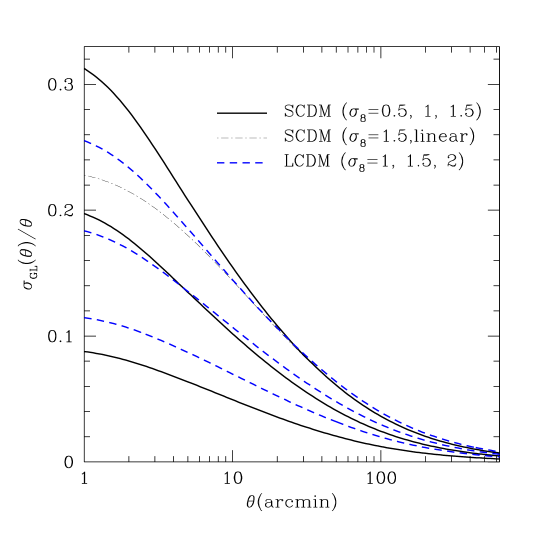
Figure 1: The dependence of $\sigma_{\rm GL}(\theta)/\theta$ on $\theta$ is shown for two cosmological models with various normalizations of CDM power spectrum and $\Omega_{\rm b0}h^{2}=0.019$. The solid lines show results of $\sigma_{8}=0.5,1.0$ and $1.5$ in SCDM ($\Omega_{\rm m0}=1$ and $h=0.5$) from bottom to top while the dashed lines are $\sigma_{8}=1.0,1.5$ and $2.0$ in LCDM ($\Omega_{\rm m0}=0.3$, $\Omega_{\rm\lambda 0}=0.7$), respectively, where the nonlinear effect on the matter power spectrum is computed using the fitting formula by Peacock & Dodds (1996). The thin dot-dashed line is for the linear power spectrum in SCDM with $\sigma_{8}=1.5$.

In Figure 1 we plot the relative lensing dispersion $\sigma_{\rm GL}(\theta)/\theta$ as a function of the separation angle $\theta$ for different sets of $\sigma_{8}$ in SCDM and LCDM models, which are computed using equations (1). The dependence of $\sigma_{8}$ in each model is demonstrated by choices of $\sigma_{8}=0.5,1$, and $1.5$ (solid lines) in SCDM, and $\sigma_{8}=1,1.5$ and $2.0$ (dashed lines) in LCDM from bottom to top, respectively. The normalizations from the COBE 4-year measurements (e.g. Bunn & White (1997)) and the X-ray cluster abundance (Eke, Cole & Frenk (1996); Kitayama & Suto (1997)) roughly correspond to $\sigma_{8}=1.2$ and $0.5$ for SCDM, and $\sigma_{8}\simeq 1-1.5$ for LCDM, respectively. Furthermore, the recent several measurements of cosmic shear (e.g. Van Waerbeke et al. (2000)) have suggested $\sigma_{8}=1.5\pm 0.5$ for the current favored LCDM models, while uncertainties involved in redshift distributions of distant galaxies, the cosmic variance of the variance of the shear and the systematic errors of the signals still remain unresolved. Figure 1 clearly shows that the magnitude of $\sigma_{\rm GL}(\theta)$ at a certain angle $\theta$ has a strong dependence on the amplitude of $\sigma_{8}$ in each cosmological model. Since the logarithmic angular power spectrum (3) of $\sigma_{\rm GL}$ has contributions from the proportional factor $\Omega^{2}_{\rm m0}$ and the distance and the growth factors, the combination yields a dependence of $\Omega_{\rm m0}$ on $\sigma_{\rm GL}(\theta)$. Although the Hubble parameter $h$ affects $\sigma_{\rm GL}$ mainly through the shape parameter $\Gamma\approx\Omega_{\rm m0}h$ in the matter power spectrum, the dependence is weaker. The thin dot-dashed line shows a result of using the linear matter power spectrum for $\sigma_{8}=1.5$ in SCDM, and it reveals that the effect of the nonlinear evolution on $\sigma_{\rm GL}$ is not important at $\theta\lower 2.15277pt\hbox{$\;\buildrel>\over{\sim}\;$}10^{\prime}$, where the two-point correlations function of hotspots has most power of correlations. It is therefore expected that the measurements of $\sigma_{\rm GL}$ can generally provide constraints on $\sigma_{8}-\Omega_{\rm m0}$ plane. To break the degeneracy between $\Omega_{\rm m0}$ and $\sigma_{8}$, we have to measure the scale dependence of $\sigma_{\rm GL}(\theta)$ with respect to $\theta$.

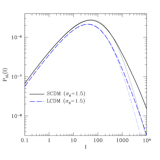
Figure 2: The logarithmic angular power spectrum of the lensing dispersion as a function of $l$ for SCDM (solid) and LCDM (dashed) models with $\sigma_{8}=1.5$ as in Figure 1. The power spectrum is computed using equation (3). The thin and thick lines in each model show the corresponding results of using linear and nonlinear three dimensional power spectrum of matter fluctuations, respectively.

As shown by equations (2) and (3), the lensing dispersion arises from the projected matter power spectrum $P_{\delta}(k)$ weighted with $a^{-2}W^{2}(\chi,\chi_{\rm rec})$. Figure 2 shows the logarithmic angular power spectrum $P_{\rm GL}(l)$ defined by equation (3) as a function of $l$. The thin and thick curves are results of using the linear and nonlinear matter power spectra, respectively, and the figure demonstrates that the nonlinear effect is important on $l\lower 2.15277pt\hbox{$\;\buildrel>\over{\sim}\;$}1000$, which corresponds to angular scales of $\theta\lower 2.15277pt\hbox{$\;\buildrel<\over{\sim}\;$}20^{\prime}$ from the relation of $l\approx 2\pi/\theta$. The shape of $P_{\rm GL}$ peaks around $l\approx 100$ and thus the contributions to the deflection angle of each CMB photon come mainly from modes with such large $l$ (see Figure 7). The essential quantity of lensing effect on $\xi_{\rm pk-pk}$ is lensing fluctuations of relative separation angle, and the term including Bessel function in $\sigma_{\rm GL,0}(\theta)$ of equation (2) indicates that the lensing fluctuations for two CMB bundles separated with a certain angle $\theta$ arises dominantly from the integrations of $P_{\rm GL}(l)$ over $l>2\pi/\theta$ in $l-$space. This physically means that the gravitational lensing effect on the relative angular separation is caused mainly by the projected matter fluctuations lied between the two bundles. Accordingly the two bundles with smaller separation are more strongly affected by the smaller scale structures of the universe. Furthermore, from these interpretations we can conclude that corrections to the flat sky approximation proposed by Hu (2000) do not affect our results at $l\lower 2.15277pt\hbox{$\;\buildrel>\over{\sim}\;$}100$ because the corrections are important only at $l<10$.

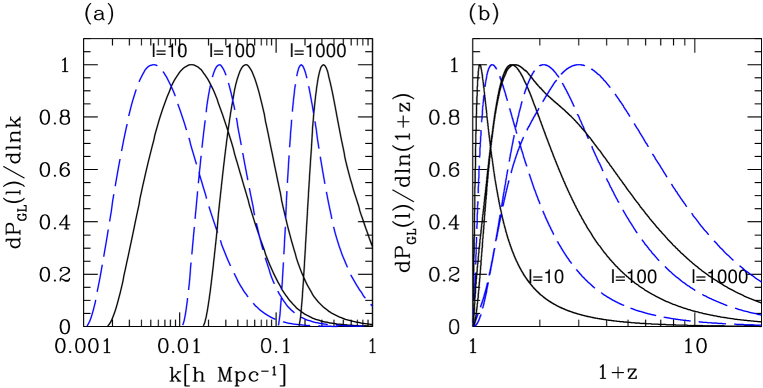
Figure 3: (a) The logarithmic contribution to the 2D power spectrum $P_{\rm GL}(l)$ defined by equation (3) as a function of $k$ for $l=10$, $100$, $1000$, where the normalization is arbitrarily scaled. The models are same as those in Figure 2. (b) The logarithmic contribution to $P_{\rm GL}(l)$ for each $l$ mode as a function of $1+z$.

Since the more fundamental quantity is the three dimensional density fluctuations characterized by the power spectrum $P_{\delta}(k)$, we have to see the relation between the two power spectra, namely $P_{\delta}(k)$ and $P_{\rm GL}(l)$. Figure 3(a) shows the logarithmic contribution to $P_{\rm GL}(l)$ for a given $l$-mode as a function of three dimensional wavenumber $k$ in the same models as in Figure 2, where normalizations of those curves are arbitrarily scaled. These functions have relatively broad shape and peaks at $\lambda=k/2\pi\approx 630h^{-1}{\rm Mpc}$ for $l=10$, at $k\approx 125h^{-1}{\rm Mpc}$ for $l=100$, and $k\approx 21h^{-1}{\rm Mpc}$ for $l=1000$ in the considered SCDM model, respectively. These relations between $l$ and $k$ depend on the shape of matter power spectrum. On the other hand, since in the LCDM model the comoving angular diameter distance at a certain redshift is larger than the corresponding distance in SCDM, the peak-wavelengths are smaller than those in the SCDM cases for each $l$ mode. The figure also demonstrates that the higher $l$ mode is affected more strongly by the matter fluctuations with smaller wavelengths.

The next question is the redshift distribution of the contribution to a given $P_{\rm GL}(l)$. Figure 3(b) shows the logarithmic contribution to $P_{\rm GL}(l)$ for each $l$ mode as a function of $(1+z)$. Since the window function $W/a$ in $P_{\rm GL}(l)$ is a monotonous decreasing function with respect to $z$ and has no characteristic redshift, the question which redshift structures give the dominant contribution depends on the shape of matter power spectrum. The figure clearly demonstrates that each curve peaks at a certain redshift; for low $l$ mode the contribution is dominated by the low-$z$ structures and, on the other hand, high $l$ mode has wide range contributions in the redshift space. These results can be explained as follows. As shown in Figure 3(a), there is the peak scale $k_{\rm max}$ of three dimensional mass fluctuations that provides most dominant contribution to $P_{\rm GL}(l)$ for each $l$ mode. Because of the projection effect on the celestial sphere, the contribution from the $k_{\rm max}$ mode comes from structures at a specific redshift $z_{\rm max}$ which satisfies the relation of $k_{\rm max}\approx l/r(z_{\rm max})$. As a result, for lower $l$ mode the contribution will be dominated by lower $z$ structures. On the other hand, for $l=1000$ mode the contribution peaks at $z\approx 0.5$ with a long tail expanding to higher $z$, where the tail is caused by the fact that the window function $W/a$ has larger power at lower $z$. In fact, Figure 3(b) confirms these interpretations. We could therefore directly probe dark matter clustering at low and high redshifts for low and high $l$ modes, respectively, in principle by using the weak lensing signatures.

4.2 Unlensed two-point correlation function of hotspots with the instrumental effects

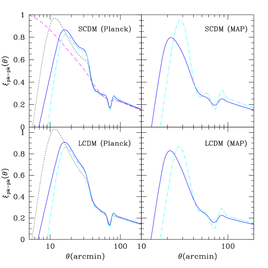
Figure 4: The unlensed two-point correlation function of hotspots of height above threshold $\nu=1$, $\xi_{\rm pk-pk}(\theta)$, as a function of the separation angle $\theta$ for SCDM (upper panels) and LCDM (bottom panels). The instrumental effects of finite beam size and detector noise for the expected Planck and MAP surveys are taken into account. The solid and dot-dashed lines shows the cases including both those effects and only the beam smearing effect, respectively. For comparison, the ideal case of $\xi_{\rm pk-pk}(\theta)$ without those effects is shown by the dotted lines in the upper left and bottom left figures. The dashed line in the upper left figure shows the conventionally used two-point correlation function $C(\theta)$ normalized to agree with the value of $\xi_{\rm pk-pk}(\theta)$ with the solid line at $\theta=200^{\prime}$.

The unlensed two-point correlation functions of local maxima (hotspots), say $\xi_{\rm pk-pk}(\theta)$, in the CMB maps can be accurately predicted based on the Gaussian random theory. The derivation is presented in the appendix B in detail. To show the shape of $\xi_{\rm pk-pk}(\theta)$, we performed a six dimensional numerical integration using equation (B5) because the two of the eight dimensional integration in equation (B5) can be analytically done. For the practical purpose, we also take into account instrumental effects of finite beam size and detector noise. The beam smearing effect on the temperature fluctuations field can be modeled by the Gaussian beam approximation characterized by a filter function $F_{l}=\exp[-l^{2}\theta_{s}^{2}/2]$ in $l$-space, where the smoothing angle $\theta_{s}$ is expressed in terms of the full-width at half-maximum angle $\theta_{\rm fwhm}$ of a telescope as $\theta_{s}=\theta_{\rm fwhm}/\sqrt{8\ln 2}$. The noise level of detectors is conventionally expressed in terms of the temperature fluctuations per a pixel on a side of FWHM extent as $\Delta_{\rm noise}=\sigma_{\rm sens}$. If we assume that the primordial temperature and the noise fields are uncorrelated, by modifying the angular power spectrum $C_{l}$ to $\tilde{C}_{l}=(C_{l}+\sigma_{\rm sens}^{2}\theta^{2}_{\rm fwhm})\exp[-l^{2}\theta_{s}^{2}]$, these instrumental effects can be approximately included into the theoretical predictions (HS), because in the Gaussian random theory $C_{l}$ contains complete information about statistical properties of any intrinsic CMB field. The numerical experiments indeed show that this treatment works well.

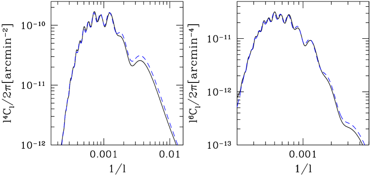
Figure 5: The logarithmic power spectra of the gradient (left) and second-derivative (right) fields of the CMB anisotropies field as a function of $1/l(\propto\theta)$. The solid and dashed lines show the results of SCDM and LCDM models, respectively. This figure clearly explains that the oscillations of $l^{2}C_{l}$ is strongly enhanced.

Figure 4 shows the unlensed $\xi_{\rm pk-pk}(\theta)$ with and without the experimental effects as a function of separation angle $\theta$ in the SCDM and LCDM models, where we considered the two hotspots of height above the threshold $\nu=1(\Delta_{\rm pk}=\sigma_{0})$. As for the instrumental effects, we have employed the specifications of Planck $217{\rm GHz}$ channel and MAP $90{\rm GHz}$ channel; the beam size and noise level are assumed to be $\theta_{\rm fwhm}=5.5^{\prime}$ and $\sigma_{\rm sens}=4.3\times 10^{-6}$ for Planck while $\theta_{\rm fwhm}=12.6^{\prime}$ and $\sigma_{\rm sens}=2.5\times 10^{-5}$ for MAP. The solid lines in each panel show $\xi_{\rm pk-pk}(\theta)$ including both effects of the beam size and noise, and the dotted lines in the upper left and bottom left panels show an ideal case without those effects. The ideal cases demonstrate that the intrinsic $\xi_{\rm pk-pk}(\theta)$ has a prominent peak at $\theta\approx 10^{\prime}$ and the damping tail at $\theta<10^{\prime}$. These features physically mean that the primary temperature field has the characteristic curvature scale of the order of $10^{\prime}$, which can be estimated by $\theta_{\ast}\equiv\sqrt{2}\sigma_{1}/\sigma_{2}\sim 5^{\prime}$ in Appendix A, and has smooth structures at scales of $\theta<\theta_{\ast}$ as actually shown by the simulated maps. The beam smearing on the intrinsic $\xi_{\rm pk-pk}(\theta)$ then appears as a cutoff at scales below the beam size although the effect moderately changes the global shape of $\xi_{\rm pk-pk}(\theta)$ in the MAP case (top right and bottom right panels). This is because the beam smearing causes an incorporation of intrinsic hotspots contained within one beam. To clarify the noise effect explicitly, we also show $\xi_{\rm pk-pk}(\theta)$ only with beam smearing effect (dot-dashed lines). The curves explain that spurious hotspots due to the detector noises generate an extra power of correlations on $\xi_{\rm pk-pk}(\theta)$. In particular, the predicted shape of $\xi_{\rm pk-pk}(\theta)$ for MAP is largely affected by the noise effect up to $\theta=80^{\prime}$ while the Planck cases have slight changes only at $\theta\lower 2.15277pt\hbox{$\;\buildrel<\over{\sim}\;$}20^{\prime}$. By using equation (A12), we can predict values of mean number density of hotspots above $\nu=1$ for those cases. The values with both the beam smearing and noise effects and only with beam effect in SCDM model are $\bar{n}_{\rm pk}=8.17\times 10^{3}$ and $7.74\times 10^{3}[{\rm rad}^{-2}]$ for Planck (upper left), respectively, while $\bar{n}_{\rm pk}=5.31\times 10^{3}$ and $3.01\times 10^{3}[{\rm rad}^{-2}]$ for MAP (upper right), respectively. Similarly, in LCDM model $\bar{n}_{\rm pk}=7.73\times 10^{3}$ and $7.33\times 10^{3}[{\rm rad}^{-2}]$ for Planck (bottom left) and $\bar{n}_{\rm pk}=5.06\times 10^{2}$ and $2.88\times 10^{3}[{\rm rad}^{-2}]$ for MAP (bottom right), respectively. These values actually coincide with results of the number counts of hotspots in the simulated CMB maps within the Poisson error. Moreover, to reveal the differences of shapes between $\xi_{\rm pk-pk}(\theta)$ and the conventionally used two-point correlation function of the temperature fluctuations field itself defined by $C(\theta)\equiv\left\langle{\Delta(\mbox{\boldmath$\theta$}_{1})\Delta(\mbox{\boldmath$\theta$}_{2})}\right\rangle_{|\mbox{\boldmath$\theta$}_{1}-\mbox{\boldmath$\theta$}_{2}|=\theta}$, the dashed line in upper left panel shows $C(\theta)$ normalized to agree with the value of solid line at $\theta=200^{\prime}$. It is clear that $\xi_{\rm pk-pk}(\theta)$ has much more oscillatory features than $C(\theta)$ does (HS; TKF). This reason is as follows. In the peak statistics we need statistical properties of the gradient and second derivative fields of the temperature fluctuations field in order to identify the local maxima (or minima) in the CMB maps. The power spectra of those fields per logarithmic interval in $l$ are then $l^{4}C_{l}/(2\pi)$ and $l^{6}C_{l}/(2\pi)$, respectively, while the power spectrum of the temperature fluctuations filed is $l^{2}C_{l}/(2\pi)$ whose integral over $l$ space produces $C(\theta)$. Figure 5 shows the power spectra of $\Delta_{,i}$ and $\Delta_{,ij}$ as a function of $1/l$ $(\propto\theta)$, and clearly explains that they strongly enhance the oscillations of $l^{2}C_{l}$. If recalling the relation of $\theta\approx 2\pi/l$, there are indeed correspondences between both oscillations of $\xi_{\rm pk-pk}(\theta)$ and $C_{l}l^{2}/(2\pi)$; the depression at $\theta\approx 70^{\prime}$ corresponding to the scales around the first Doppler peak, a prominent peak at $\theta\approx 13^{\prime}$, and a damping tail at $\theta<10^{\prime}$ associated with the Silk damping in $C_{l}$. Most importantly, these oscillatory features of $\xi_{\rm pk-pk}(\theta)$ physically mean that pairs of hotspots are discretely distributed with some characteristic separation angles on the last scattering surface. The peak statistics thus produces an additional information that could be convenient for the study of the weak lensing although it relys on only a subset of available information (the location of peaks, peak height and their profile). Furthermore, we expect that the distribution of hotspots are more robust against the systematic observational errors. The previous works already concluded that the lensing effect on $C_{l}$ is small at $l<3000$ (e.g. see Seljak 1996 and references therein), and we therefore expect that the observed $C_{l}$ will provide the accurate prediction of unlensed $\xi_{\rm pk-pk}(\theta)$. The lensing signatures to $\xi_{\rm pk-pk}(\theta)$ are then extracted as non-Gaussian signatures, which are differences between the observed (lensed) and the predicted two-point correlation functions.

4.3 Lensed two-point correlation function of hotspots

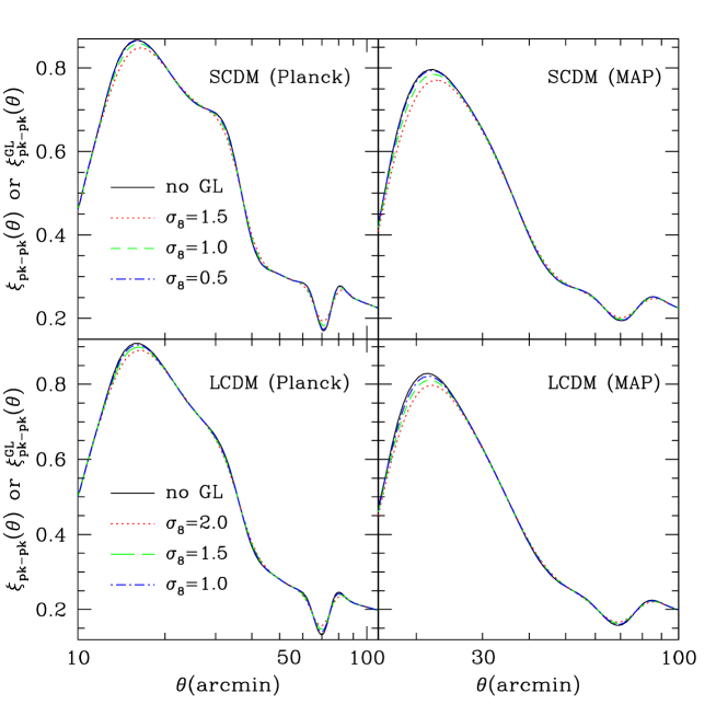
Figure 6: The lensed and unlensed two-point correlation functions of hotspots as a function of $\theta$ using the same parameters of experimental effects as those in Figure 4. The weak lensing effects are computed using the same models of matter power spectrum with sets of $\sigma_{8}$ as in Figure 1.

We present the theoretical predictions of the lensed two-point correlation function of hotspots. By using equation (9) we then compute the lensing effect on the intrinsic $\xi_{\rm pk-pk}(\theta)$ into which the experimental effects are already included by the method presented in the previous subsection. Although the order of computing those secondary effects is not correct, the treatment makes the calculations much simpler and is a good approximation because of the following reasons. As explained, the instrumental effects on $\xi_{\rm pk-pk}(\theta)$ can be approximately included only by modifying the angular power spectrum $C_{l}$ based on the Gaussian theory and actually the predictions are in good agreement with the numerical experiments of $\xi_{\rm pk-pk}(\theta)$ (HS and also see Figure 8). This means that the distribution of hotspots as a point process can be accurately predicted even in the CMB maps altered by the beam smearing and the detector noise. Then, since we are here interested in a problem how the weak lensing redistributes the ‘key’ hotspots, which can survive after the beam smearing effect, in an actual observed map, we can approximately consider the lensing effect on the $\xi_{\rm pk-pk}(\theta)$ after the instrumental effects as long as the weak lensing does not create a lot of spurious hotspots on the map. Moreover, we can at least say that the important lensing signature to $\xi_{\rm pk-pk}$ on large angular scales such as $\theta\approx 70^{\prime}$ is not directly coupled to the beam smearing effect of $\theta_{\rm fwhm}\lower 2.15277pt\hbox{$\;\buildrel<\over{\sim}\;$}10^{\prime}$. The validity of our treatment has been confirmed by the numerical experiments on the relevant angular scales. Figure 6 shows both unlensed and lensed two-point correlation functions of hotspots, say $\xi_{\rm pk-pk}^{\rm GL}(\theta)$ and $\xi_{\rm pk-pk}(\theta)$, where the threshold $\nu=1$ is similarly assumed and we employ the same models of matter power spectrum as in Figure 1. Although $\nu=1$ is assumed throughout this paper for simplicity, the two-point correlation function of hotspots above height of an arbitrary threshold can be predicted under the Gaussian theory and we could use this freedom for measuring the lensing effect as will be discussed later. The upper left and bottom left panels for Planck case clearly demonstrate that the weak lensing effect fairly smooths out the shape of unlensed $\xi_{\rm pk-pk}(\theta)$ (solid line). The magnitude of the lensing effect is strongly sensitive to the amplitude of $\sigma_{8}$ in each cosmological models and larger at angular scales where $\xi_{\rm pk-pk}(\theta)$ has more oscillatory features (TKF). In particular, we stress that the weak lensing causes a distinct smoothing effect on the depression feature of $\xi_{\rm pk-pk}(\theta)$ at scales around $\theta\approx 70^{\prime}$. We therefore expect that the observed depth of depression relative to the plateau shape at larger or smaller scales than the scale can be a robust indicator of the weak lensing signatures and depends only on the magnitude of $\sigma_{\rm GL}$ if it is large sufficiently to detect. However, since in the MAP cases (upper right and bottom right panels) the detector noise effect decreases largely the depth of the intrinsic depression as shown in Figure 4, the lensing effect is hidden at the scale for all models. If using the relation between $k$ and $l$ shown in Figure 3(a), the measure of $\sigma_{\rm GL}(\theta)$ from the lensing signature at $\theta\approx 70^{\prime}$ can provide a constraint on the amplitude of mass fluctuations with large wavelength modes such as $\lambda\approx 50h^{-1}{\rm Mpc}$. On the other hand, the measurement of $\sigma_{\rm GL}$ at the prominent peak scale such as $\theta\approx 20^{\prime}$ is sensitive to the smaller scale structures such as $\lambda\approx 10h^{-1}{\rm Mpc}$, while the shape of $\xi_{\rm pk-pk}$ is also sensitive to the experimental effects at such scales.

5 Detectability of the lensing signatures

In this section, by using numerical experiments we quantitatively investigate how accurately non-Gaussian signatures on $\xi_{\rm pk-pk}(\theta)$ induced by the weak lensing can be detected with the expected future MAP and Planck surveys.

5.1 Numerical experiments

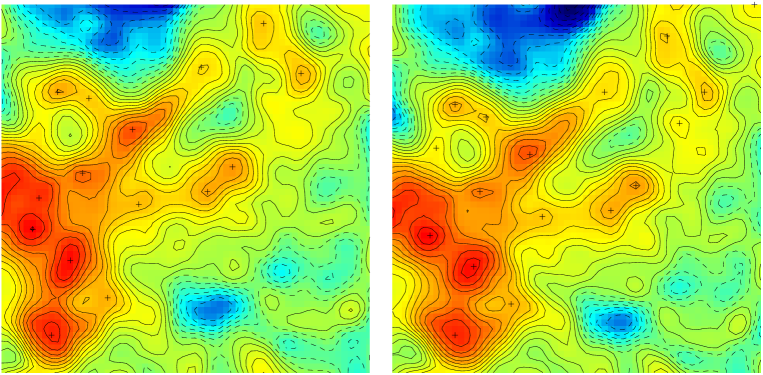
Figure 7: An example of simulations of primordial temperature fluctuations map (left) and the map deformed by the lensing effect (right) on a side of $2$ degree, where we assumed the instrumental resolutions of Planck ($\theta_{\rm fwhm}=5.5^{\prime}$ and $\sigma_{\rm sens}=4.3\times 10^{-6}$). We employed the SCDM model and the lensing displacements field is computed by using $\sigma_{8}=1.5$. The peaks above $1\sigma$ are marked with crosses and the contours are stepped in units of $3\sigma_{\rm sens}$.

We perform simulations of the CMB maps with and without the lensing effect by using the following procedures. A realistic unlensed temperature maps on a fixed square grid can be generated from a given power spectrum, $C_{l}$, based on the Gaussian assumption. Each simulated map is initially on $40\times 40$ square degree area with $4096\times 4096$ pixels. After regridding to take into account the beam smearing effect, the actual pixel number is reduced to $1200\times 1200$ and $480\times 480$ for the Planck and MAP cases, respectively. To compute the lensing effect on the CMB maps, we first need the convergence field on each grid. We then employ the following angular power spectrum of convergence field (Blandford et al. (1991); Miralda-Escude (1991); Kaiser (1992));

$$P_{\kappa}(l)=\frac{9}{4}H_{0}^{4}\Omega_{\rm m0}^{2}\int^{\chi_{\rm rec}}_{0}\!\!d\chi a^{-2}W^{2}(\chi,\chi_{\rm rec})P_{\delta}\left(k=\frac{l}{r(\chi)},\chi\right),$$ (10)

where the convergence field $\kappa$ is expressed in terms of the radial integral of three dimensional density fluctuations field $\delta$ as $\kappa=(3/2)H_{0}^{2}\Omega_{\rm m0}\int\!d\chi W(\chi,\chi_{\rm rec})r(\chi)a^{-1}\delta$. Note that the second moment of convergence field is then $\left\langle{\kappa^{2}(\mbox{\boldmath$\theta$})}\right\rangle=\int(ldl/2\pi)P_{\kappa}(l)$. Using the power spectrum $P_{\kappa}(l)$, the convergence field can be generated as a realization of a Gaussian process. To compute the displacement vector $\delta\mbox{\boldmath$\theta$}$, we transform the convergence field in the Fourier space, and compute the Fourier component of the displacement vector, $\delta\tilde{\mbox{\boldmath$\theta$}}(\mbox{\boldmath$l$})$, by using the relation of

$$\delta\tilde{\mbox{\boldmath$\theta$}}(\mbox{\boldmath$l$})=2i\frac{\mbox{\boldmath$l$}}{l^{2}}\tilde{\kappa}(\mbox{\boldmath$l$}),$$ (11)

where we have used the relation of $2\kappa(\mbox{\boldmath$\theta$})=\partial(\delta\theta_{1})/\partial\theta_{1}+\partial(\delta\theta_{2})/\partial\theta_{2}$ derived by the cosmological lens equation. If transforming it back to real space, for each point on the observed temperature map we can obtain the corresponding displacement vector to map the point on a irregular grid of the primary temperature map on the last scattering surface. The lensed temperature map can be then obtained by using cloud-in-cell interpolation to compute the value on the original regular grid of observed map. In the case of taking into account the instrumental effects of beam smearing and noise, we furthermore smooth out the temperature map by convolving the Gaussian window function ${\cal F}(\mbox{\boldmath$\theta$},\mbox{\boldmath$\theta$}^{\prime})=1/(2\pi\theta_{s}^{2})\exp[-|\mbox{\boldmath$\theta$}-\mbox{\boldmath$\theta$}^{\prime}|^{2}/(2\theta_{s}^{2})]$ and then add randomly the noise field into each pixel. Figure 7 illustrates an example of realizations of the simulated unlensed and lensed maps for the SCDM model with $\sigma_{8}=1.5$, which provides the largest lensing signatures of our considered models. Interestingly, the figure shows that the displacement of each position of hotspots in the lensed map from the unlensed map is relatively large even though the global patterns of temperature fluctuations in both maps are not considerably changed. This is the consequence of the large scale modes of the deflection angle, which play an important role to the lensing effect on $\xi_{\rm pk-pk}(\theta)$.

5.2 The signal to noise ratio of the lensing signatures

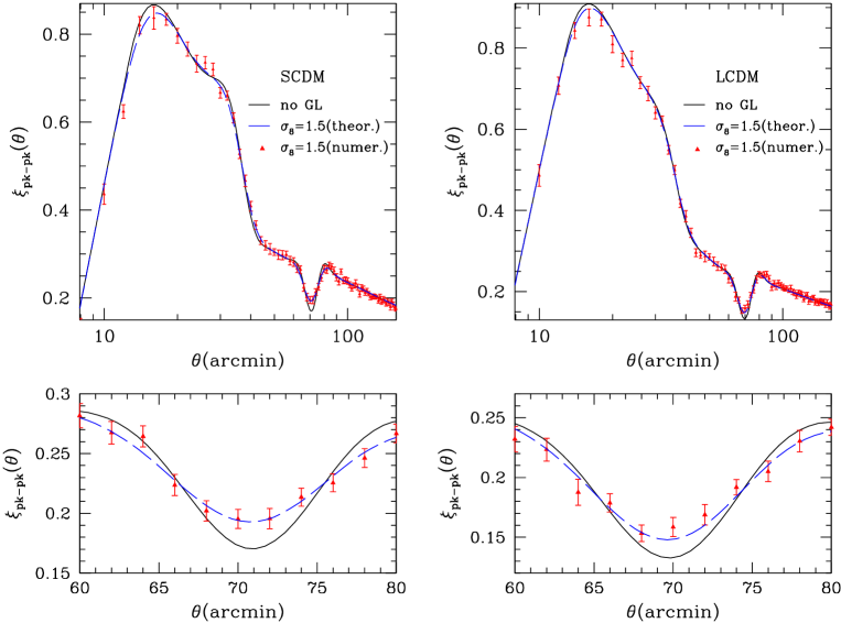
Figure 8: An example of averaged two-point correlation function with lensing effect expected from Planck survey in SCDM (left) and LCDM (right) models with $\sigma_{8}=1.5$, respectively. The solid and dashed lines show the theoretical predictions of unlensed and lensed $\xi_{\rm pk-pk}(\theta)$ as in Figure 4 and 6, respectively. The numerical results are obtained from one set of 17 realizations of the lensed maps, and the error bars correspond to the cosmic variance computed from $100$ realizations. The bottom panels show the results around the depression angular scale ($\approx 70^{\prime}$) of the unlensed $\xi_{\rm pk-pk}(\theta)$.

The observational errors associated with measurements of $\xi_{\rm pk-pk}(\theta)$ arise from the cosmic variance and the instrumental resolutions. To accurately compute the cosmic variance, we have used $100$ independent realizations of both unlensed and lensed temperature maps, respectively, with $40\times 40$ square degree area. In this paper we assume $65\%$ sky coverage for MAP and Planck surveys, and this corresponds to the assumption that we can use about $17$ independent simulated maps for those surveys in order to obtain the averaged $\xi_{\rm pk-pk}(\theta)$. In Figure 8 we show an example of the averaged lensed two-point correlation functions of hotspots computed from one set of 17 realizations for the expected Planck runs, where the error-bars in each bin can be estimated by rescaling the variance of the estimates obtained from the $100$ realizations by a factor of $\sqrt{17}$ and the resolution of bins in $\theta$ is limited by the pixel size of simulated CMB maps. The unlensed cases have been already presented by HS. The bottom panels also show the results around the depression scale $\theta\approx 70^{\prime}$ of $\xi_{\rm pk-pk}(\theta)$ in each cosmological model. Figure 8 clearly shows that the theoretical predictions are in remarkable good agreement with the numerical results. In particular, the lensing signatures at the depression scale definitely deviate from the unlensed cases, and we therefore expect that the non-Gaussian signatures should be detected by Planck with high significance for some adequate values of $\sigma_{8}$. On the other hand, for the lensing signatures at smaller scales such as the prominent scale $\theta\approx 20^{\prime}$, it seems to be slightly difficult to distinguish them because the sampling variance are larger at smaller scales and the shapes of $\xi_{\rm pk-pk}(\theta)$ is also sensitive to the instrumental effects of beam smearing and noise as shown in Figure 4. On the other hand, we concluded that it is difficult for MAP survey to distinguish the lensing signatures on $\xi_{\rm pk-pk}(\theta)$ for all cosmological models considered in this paper. For this reason, we present only results from Planck in the following.

We so far have adopted the specific shape of matter power spectrum in each considered cosmological model, and therefore a free parameter of our model is only $\sigma_{8}$. While the actual observable quantity of our method is the lensing dispersion $\sigma_{\rm GL}(\theta)$, we here investigate the dependence of the lensing signatures to $\xi_{\rm pk-pk}(\theta)$ on $\sigma_{8}$ for simplicity and the problem will be discussed in the final section. In Table 1 we summarize the results obtained for the determination of $\sigma_{8}$ with a best fit and the error associated with this determination. The error then has been determined as the variance of the best fit values of $\sigma_{8}$ among a lot of sets of the numerical experiments performed by fitting the simulated results to the theoretical templates of lensed $\xi_{\rm pk-pk}(\theta)$ so that the $\chi$-square is minimum. Each best fit of theoretical curves to the numerical experiments is restricted mainly from the data at $\theta>20^{\prime}$, in particular the data around the depression scale of $\xi_{\rm pk-pk}(\theta)$. One can see that the signal to noise ratio indeed grows with $\sigma_{8}$ in each cosmological model. Furthermore, if comparing results obtained from SCDM and LCDM models with the same value of $\sigma_{8}$ ($\sigma_{8}=1.5$), it is clear that more robust constraints can be provided in SCDM, more generally for background models with larger $\Omega_{\rm m0}$, as expected. The noise level of Planck is independent on the $\sigma_{8}$ estimations, but we have confirmed that the beam size is rather important for the detections. Importantly, the accuracies of $\sigma_{8}$ determinations expected from Planck reach about $8\%$ and $11\%$ for models with $\sigma_{8}=1.5$ in SCDM and LCDM, respectively. Furthermore, in the Gaussian random theory the two-point correlation function of local minima (coldspots) should have the same shape as that of hotspots, and therefore combing the measurements of coldspots correlation function improves the lensing signals by about factor $\sqrt{2}$. We could also improve the significance by combining the measurements of $\xi_{\rm pk-pk}$ with another different thresholds, but the independence of data then has to be carefully investigated because the angular positions of same hotspots are used many times in the fitting.

Table 1: Summary of best fit of $\sigma_{8}$ determinations from the lensing signatures to $\xi_{\rm pk-pk}(\theta)$ using the numerical experiments for the expected Planck survey in SCDM and LCDM models. We have assumed $65\%$ sky coverage, and the $1\sigma$ error in each determination represents uncertanities caused by the cosmic variance and the instrumental effects due to the beam smearing effect and the detector noise (see text).

input values of $\sigma_{8}$	SCDM $(\Omega_{\rm m0}=1,h=0.5)$	LCDM $(\Omega_{\rm m0}=0.3,\Omega_{\rm\lambda 0}=0.7,h=0.7)$
0	$0.30\pm 0.31$	$0.23\pm 0.35$
0.5	$0.47\pm 0.24$	-
1.0	$1.03\pm 0.13$	$0.93\pm 0.23$
1.5	$1.52\pm 0.12$	$1.49\pm 0.17$
1.5 (without noise)	$1.47\pm 0.12$	$1.53\pm 0.16$
2.0	-	$1.97\pm 0.16$

Our arguments presented in this section rely on the expectation that we can accurately predict the shape of unlensed $\xi_{\rm pk-pk}(\theta)$ as a function of sets of cosmological parameters constrained from the measured angular power spectrum $C_{l}$ within the limit of the observational errors. However, we should bear in mind the fact that only the lensed $C_{l}$ is measurable. Then, one may imagine an approach to compare the measured $\xi_{\rm pk-pk}$ to the fake prediction, say $\tilde{\xi}_{\rm pk-pk}$, computed directly from the lensed (measured) $C_{l}$ based on the Gaussian theory. Since the lensed temperature fluctuations field weakly deviates from the Gaussian (Bernardeau (1997)), the distribution of hotspots in the lensed maps can be no longer characterized only by the lensed $C_{l}$. However, it will be still interesting to see differences between the exact and fake predictions of the lensing effect on $\xi_{\rm pk-pk}(\theta)$. Figure 9 thus shows the shape of $\tilde{\xi}_{\rm pk-pk}$ and reveals that $\tilde{\xi}_{\rm pk-pk}$ overestimates the power of correlations on scales of $\theta<40^{\prime}$, while $\tilde{\xi}_{\rm pk-pk}$ mimics the smoothing effect on the depression feature of $\xi_{\rm pk-pk}$ resulting from the fact that the weak lnsing already causes the smoothing of $C_{l}$. Consequently, for example, the value of reduced $\chi$-square for the fitting between $\tilde{\xi}_{\rm pk-pk}$ and the simulated $\xi_{\rm pk-pk}$ becomes worse to be $\chi^{2}\approx 162/95$ against the fact that the fitting of using the exact theoretical predictions (9) of lensed $\xi_{\rm pk-pk}$ produces values around almost unity. Hence, the important problem how we extract the lensing information only from the measurable CMB quantities has to be carefully investigated and this problem will be again discussed in the next section.

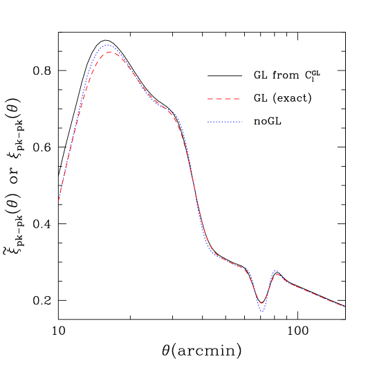
Figure 9: This figure shows the fake theoretical predction of lensed hotspots correlation function (solid line), $\tilde{\xi}_{\rm pk-pk}$, computed from the lensed (measured) $C_{l}$ based on the Gaussian theory in the SCDM model with $\sigma_{8}=1.5$. The exact prediction (dashed line) and the unlnesed case (dotted line) are also shown. Since the lensed temprature fluctuations field weakly deviates from the Gaussian, $\tilde{\xi}_{\rm pk-pk}$ can no longer accurately describe the distribution of hotspots in the lensed maps.

6 Discussion and Conclusions

In this paper, we have quantitatively shown that the peak-peak correlation function for the CMB maps can be an efficient measure to probe the mass fluctuations at relatively large scales. The non-Gaussian signatures on $\xi_{\rm pk-pk}(\theta)$ caused by the weak lensing appear at several scales as smoothing effects on the oscillatory features of $\xi_{\rm pk-pk}(\theta)$ (TKF). In particular, by using numerical experiments of the CMB maps including effects of beam smoothing and detector noise as well as the lensing displacements, we found that the lensing signatures at about one degree scales, where the intrinsic $\xi_{\rm pk-pk}(\theta)$ has the pronounced depression feature, should be detected most significantly from the expected Planck survey if the signatures are adequately large for the detections. On the other hand, unfortunately we concluded that it is difficult for MAP to detect the lensing signatures for the cosmological models considered in this paper. The direct observable quantity of our method is the dispersion of lensing deflection angle as shown by equation (9). We have then revealed that the one-degree scale dispersions are sensitive to amplitudes of three dimensional mass fluctuations around wavelength $\lambda\approx 50h^{-1}{\rm Mpc}$ because of the projection effect. Furthermore, such lensing dispersions have contributions from structures of the universe with a wide redshift distribution in the range of $1\lower 2.15277pt\hbox{$\;\buildrel<\over{\sim}\;$}z\lower 2.15277pt\hbox{$\;\buildrel<\over{\sim}\;$}3$ (see Figure 3). This projection effect would be thus a serious issue for extracting the cosmological information from weak lensing contributions in a general case. However, since the mass fluctuations around $\lambda\sim 50h^{-1}{\rm Mpc}$ are now still in the linear regime and the evolution history in the redshift space is theoretically well understood in the context of gravitational instability in an expanding universe, the lensing signatures can accurately determine the cosmological parameters associated with amplitude and evolution of mass fluctuations at the scales. It is therefore expected that our method can provide robust constraints on cosmological parameters $\sigma_{8}$ and $\Omega_{\rm m0}$ without much specifying the shape of matter power spectrum. Our numerical experiments indeed revealed that significant signal to noise rations for determinations of $\sigma_{8}$ from the lensing signatures to $\xi_{\rm pk-pk}(\theta)$ are obtained for some input values of $\sigma_{8}$ in SCDM and LCDM models, respectively. It was also shown that for the same value of $\sigma_{8}$ more significant signal can be obtained in SCDM than in LCDM. To break the degeneracy in $\sigma_{8}-\Omega_{\rm m0}$ determinations only by using our method, one must measure the scale dependence of lensing signatures. This seems to be difficult even for Planck survey, because the shape of $\xi_{\rm pk-pk}(\theta)$ at small scales of $\theta\approx 20^{\prime}$ where $\xi_{\rm pk-pk}$ has the secondly significant lensing signatures is also sensitive to the instrumental effects of beam smoothing and noise. Anyway, it is very interesting that our method could provide constraints on the mass fluctuations in the linear regime independently of those provided by the survey of galaxies clustering and the primary CMB anisotropies alone, which cannot directly probe the power spectrum of dark matter.

In the results presented in this paper, we have discussed how accurately the non-Gaussian signatures of the lensed $\xi_{\rm pk-pk}^{\rm GL}$ can be detected as a deviation from the unlensed $\xi_{\rm pk-pk}$ as shown in Figure 8. This strategy is based on the assumption that we can accurately predict the unlensed $\xi_{\rm pk-pk}(\theta)$ from the measured $C_{l}$ because the lensing effect on $C_{l}$ is small (Seljak 1996b ). However, since an actual measurable quantity is only the lensed $C_{l}$, there remains an important problem that we have to carefully investigate. Usually, the measured angular power spectrum $C_{l}$ can be used to constrain the sets of cosmological parameters under a specific scenario, for example, within the framework of inflationary-motivated models (e.g. Lange et al. (2000)). The detailed analysis of using higher $l$ modes such as $l>3000$ will need to take into account the lensing contributions to $C_{l}$ for the accurate determinations (Stompor & Efstathiou (1999)). Therefore, one approach toward detecting the lensing effect on $\xi_{\rm pk-pk}$ is that we first construct a lot of templates of the unlensed $\xi_{\rm pk-pk}$ as a function of sets of cosmological parameters constrained by the measured $C_{l}$ within the observational errors, and then we compare the templates with the directly measured $\xi_{\rm pk-pk}$ in the observed (lensed) CMB maps by taking into account the lensing contributions. Based on the considerations, we are now investigating the detailed dependence of cosmological parameters on the shape of $\xi_{\rm pk-pk}$. As a result, we confirm to a extent that, if we focus on the depth of depression feature of $\xi_{\rm pk-pk}(\theta)$ at one degree scales relative to the plateau shapes at larger or smaller scales than that scale, the measured depth could be a robust indicator relatively independently of the cosmological parameters because the weak lensing with same magnitude of $\sigma_{\rm GL}$ can shallow the measured depth to a same amount. This should be further investigated carefully and will be presented elsewhere. The important thing that we stress in this paper is that we quantitatively proposed a new statistical method for measuring the lensing effect based on the peak statistics. It is not evident that our method and the other methods can measure the small lensing signatures from the observed CMB data with exactly same statistical significance. Therefore, several independent methods should be performed to measure the lensing signatures complementarily.

Undoubtedly, we have to carefully consider how secondary anisotropies and the foreground sources affect our conclusions. The most important source of secondary anisotropies is the (thermal) Sunyaev-Zel’dovich (SZ) effect, which is essentially caused by hot electrons inside the clusters of galaxies. Since SZ induces redistributions of the photon energy from low frequency to high frequency part of the black body spectrum, the effect could mimic peaks in the observed temperature map. However, the SZ anisotropies are dominated by the Poisson contribution from the individual clusters at relevant angular scales (Komatsu & Kitayama (1999)), and therefore the contribution of the cross correlation between spurious peaks due to SZ and the intrinsic peaks will be smaller than the amplitude of the intrinsic peak-peak correlation because the peaks on the last scattering surface and the SZ clusters are statistically uncorrelated. Furthermore, we should emphasize that the SZ effect can be always removed by either observing at $217$ GHz or by taking advantage of its specific spectral properties. The other secondary anisotropies such as Rees-Sciama effect do not affect our method because the amplitudes of those effects have a very small contribution at $l<3000$ (Seljak 1996a ). Finally, with regard to the effect of the extragalactic sources, since it is expected that the amplitude of anisotropies due to the discrete sources in the $100-200$ GHz range are well bellow the amplitude of primordial fluctuations (Toffolatti et al. (1998)) and the sources will be also eliminated by using the multi frequency observations in principle, it can be safely concluded that this is not a serious for our method.

Recent measurements of cosmic shear (e.g. see Van Waerbeke et al. (2000)) have provided constraints on the combination of $\sigma_{8}$ and $\Omega_{\rm m0}$. The cosmic shear can probe the mass fluctuations at angular scales of $1^{\prime}\lower 2.15277pt\hbox{$\;\buildrel<\over{\sim}\;$}\theta\lower 2.15277pt\hbox{$\;\buildrel<\over{\sim}\;$}30^{\prime}$ because of the limited survey volume, where the nonlinear clustering effect of dark matter could play an important role. It has been also shown that the deformation effects on the CMB maps could be measured by Planck (Bernardeau (1998); Waerbeke, Bernardeau & Benabed (1999)), and it is sensitive to the projected mass fluctuations at scales around $5^{\prime}$ which is the characteristic curvature scale of the primary temperature field. Therefore, although $\Omega_{\rm m0}$ parameter cannot be determined accurately form the primary CMB anisotropies alone even with Planck because of the so-called cosmic (geometrical) degeneracy (Bond, Efstathiou, & Tegmark (1997)), it is expected that our method and those other independent methods of using the weak lensing will break the cosmic degeneracy with high precision because the amplitude of lensing contributions is also sensitive to $\Omega_{m0}$ as explained. Another challenging possibility is that those independent methods could allow us to observationally reconstruct the shape of power spectrum of dark matter including the evolution history in the redshift space by combining those measurements of amplitudes of mass fluctuations at respective angular scales.

Appendix A Mean density of hotspots in the 2D CMB map

In this appendix, we briefly review the derivation of the mean number density of peaks in the two dimensional Gaussian field (Bardeen et al. (1986); Bond & Efstathiou (1987)).

Following BBKS and BE, we introduce the spectral parameters defined by

$$\gamma\equiv\frac{\sigma_{1}^{2}}{\sigma_{0}\sigma_{2}},\hskip 40.00006pt\theta_{\ast}=\sqrt{2}\frac{\sigma_{1}}{\sigma_{2}},$$ (A1)

where

$$\sigma_{n}^{2}\equiv\int\!\!\frac{ldl}{2\pi}C_{l}l^{2n}.$$ (A2)

The characteristic curvature scale of primary temperature field can be estimated as $\theta_{\ast}\sim 5^{\prime}$ for the cosmological models considered in this paper.

The problem of the two dimensional peak statistics is to consider the statistical properties of the point process. We can then express the point process entirely in terms of the field and its derivatives. At hotspots (coldspots) the gradient $\Delta_{i}(\equiv\partial\Delta/\partial\theta^{i})$ vanishes, and the eigenvalues of curvature matrix $\Delta_{ij}(\equiv\partial^{2}\Delta/(\partial\theta^{i}\partial\theta^{j}))$ are all negative (positive). We therefore need to consider six independent variables $\mbox{\boldmath$v$}=(\Delta,\Delta_{x},\Delta_{y},\Delta_{xx},\Delta_{yy},\Delta_{xy})$ to specify one local maximum. For the Gaussian field, the probability density function (PDF) for $v$ is

$$p_{1}(\mbox{\boldmath$v$})=\frac{1}{(2\pi)^{3}|{\rm det}(M_{ij})|^{1/2}}\exp\left(-\frac{1}{2}v_{i}M^{-1}_{ij}v_{j}\right),$$ (A3)

where the covariance matrix is $M_{ij}=\left\langle{v_{i}v_{j}}\right\rangle$ because of $\left\langle{v_{i}}\right\rangle=0$ in the present case, and $M^{-1}_{ij}$ is the inverse matrix of $M_{ij}$. Following HS, we introduce the notations for convenience as

$$\nu\equiv\frac{\Delta}{\sigma_{0}},\hskip 20.00003pt\eta_{i}\equiv\frac{\Delta_{i}}{\sigma_{1}}\ (i=x,y)$$

$$X\equiv-\frac{\Delta_{xx}+\Delta_{yy}}{\sigma_{2}},\hskip 20.00003ptY\equiv\frac{\Delta_{xx}-\Delta_{yy}}{\sigma_{2}},\hskip 20.00003ptZ\equiv\frac{2\Delta_{xy}}{\sigma_{2}}.$$ (A4)

The non-zero second moments of these variables are

$$\left\langle{\nu^{2}}\right\rangle=\langle{X^{2}}\rangle=2\langle{Y^{2}}\rangle=2\langle{Z^{2}}\rangle=2\left\langle{\eta_{i}^{2}}\right\rangle=1,\hskip 10.00002pt\langle{\nu X}\rangle=\gamma,$$ (A5)

where $\gamma\equiv\sigma_{1}^{2}/(\sigma_{0}\sigma_{2})$. By using these equations, we can obtain the following PDF for the variables $\mbox{\boldmath$v$}=(\nu,X,Y,Z,\eta_{i})$ with the simple form, and it gives a probability that the field point has values in the ranges of $\nu$ to $\nu+d\nu$, $X$ to $X$ to $X+dX$ and so on:

$$p_{1}(\nu,X,Y,Z,\mbox{\boldmath$\eta$}_{i})d\nu dXdYdZd^{2}\eta_{i} = \frac{2^{2}}{(2\pi)^{3}\sqrt{1-\gamma^{2}}}\exp\left[-Q\right]d\nu dXdYdZd^{2}\eta_{i}$$ (A6)

with

$$2Q=\frac{(\nu-\gamma X)^{2}}{1-\gamma^{2}}+X^{2}+2Y^{2}+2Z^{2}+2\mbox{\boldmath$\eta$}^{2}.$$ (A7)

The point process of hotspots (or coldspots) can be described by the number density ‘operator’

$$n_{\rm pk}(\mbox{\boldmath$\theta$})=\sum_{p}\delta^{D}(\mbox{\boldmath$\theta$}-\mbox{\boldmath$\theta$}_{{\rm pk},p}),$$ (A8)

where $\delta^{D}(x)$ is the Dirac delta function. In the neighborhood of a hotspot point $\mbox{\boldmath$\theta$}_{\rm pk}$ we can expand the field $\Delta(\mbox{\boldmath$\theta$})$ in a Taylor series:

$$\Delta(\mbox{\boldmath$\theta$})\approx\Delta(\mbox{\boldmath$\theta$}_{\rm pk})+\frac{1}{2}\Delta_{ij}(\mbox{\boldmath$\theta$}_{\rm pk})(\theta-\theta_{\rm pk})_{i}(\theta-\theta_{\rm pk})_{j}.$$ (A9)

Using this equation, therefore, the number density field can be expressed in terms of the Gaussian variables:

$$n_{\rm pk}(\mbox{\boldmath$\theta$})=|{\rm det}(\Delta_{ij}(\mbox{\boldmath$\theta$}))|\delta^{D}(\Delta_{i}(\mbox{\boldmath$\theta$})).$$ (A10)

The summation symbol in equation (A8) can be eliminated because the delta function of the above equation picks out all of the extremal points which are zero of $\Delta_{i}(\mbox{\boldmath$\theta$})$ are maximum in the two dimensional map.

Hence the ensemble average of equation (A10) produces the differential mean number density of hotspots of height in the range of $\nu$ and $\nu+d\nu$:

$$\bar{n}_{\rm pk}(\nu) = \left\langle{|{\rm det}(\Delta_{ij})|\delta^{D}(\Delta_{i})}\right\rangle=\frac{1}{2\theta_{\ast}^{2}}\left\langle{|X^{2}-Y^{2}-Z^{2}|\delta^{D}(\eta_{i})}\right\rangle$$ (A11)

$$= \frac{1}{2\theta_{\ast}^{2}}\int^{\infty}_{0}\!\!dX\int^{X}_{-X}\!\!dY\int^{\sqrt{X^{2}-Y^{2}}}_{-\sqrt{X^{2}-Y^{2}}}dZ(X^{2}-Y^{2}-Z^{2})p_{1}(\nu,X,Y,Z,\eta_{i}=0),$$

where we have adopted the conditions for a hotspot of $X>0$ and $Y^{2}+Z^{2}<X^{2}$. BE derived the analytical expression for $\bar{n}_{\rm pk}(\nu)$;

$$\bar{n}_{\rm pk}(\nu)=\frac{1}{(2\pi)^{3/2}\theta^{2}_{\ast}}\exp(-\nu^{2}/2)G(\gamma,\gamma\nu),$$ (A12)

where

$$G(\gamma,x_{\ast}) \equiv (x_{\ast}^{2}-\gamma^{2})\left\{1-\frac{1}{2}{\rm erfc}\left[\frac{x_{\ast}}{\sqrt{2(1-\gamma^{2})}}\right]\right\}+x_{\ast}(1-\gamma^{2})\frac{\exp\{-x_{\ast}^{2}/[2(1-\gamma^{2})]\}}{\sqrt{2\pi(1-\gamma^{2})}}$$ (A13)

$$+\frac{\exp[-x_{\ast}^{2}/(3-2\gamma^{2})]}{(3-2\gamma^{2})^{1/2}}\left\{1-\frac{1}{2}{\rm erfc}\left[\frac{x_{\ast}}{\sqrt{2(1-\gamma^{2})(3-2\gamma^{2})}}\right]\right\}.$$

In this paper, we have often used the mean number density of peak of height above a certain threshold $\nu_{\rm thresh}$ obtained by integrating equation (A12) over $\nu>\nu_{\rm thresh}$. Naturally, the mean number density of coldspots of height below $-\nu$ ($\Delta_{\rm pk}<-\nu\sigma_{0}$) is symmetrically given by $\bar{n}_{\rm cold}(<-\nu)=\bar{n}_{\rm pk}(>\nu)$.

Appendix B The unlensed two-point correlation function of hotspots

Based on the peak statistics for the two dimensional Gaussian field, we briefly review the derivation of two-point correlation function of hotspots following HS. For this purpose, let us consider two hotspots separated by the angular scale $\theta$. In the same way as in appendix A, we then need the joint probability density function for the 12 independent variables $\mbox{\boldmath$v$}=(\mbox{\boldmath$v$}_{1},\mbox{\boldmath$v$}_{2})=(\mbox{\boldmath$v$}(\mbox{\boldmath$\theta$}_{1}),\mbox{\boldmath$v$}(\mbox{\boldmath$\theta$}_{2}))$ with $\theta=|\mbox{\boldmath$\theta$}_{1}-\mbox{\boldmath$\theta$}_{2}|$. If using the variables (A4) for each hotspot, we can block the covariance matrix $M_{ij}$ for the 12 variables in the order $(\nu_{1},X_{1},\eta_{1x},Y_{1},\nu_{2},X_{2},\eta_{2x},Y_{2},\eta_{1y},\eta_{2y},Z_{1},Z_{2})$ into the $8\times 8$-matrix $M_{(8)}$ (upper left) and the $4\times 4$-matrix $M_{(4)}$ (bottom right);

$$M_{(8)}=\left(\begin{array}[]{cccccccc}1&\tilde{\gamma}&0&0&\lambda_{000}&\lambda_{020}&-\lambda_{011}&\lambda_{022}\\ \ddots&1&0&0&\lambda_{020}&\lambda_{220}&-\lambda_{121}&\lambda_{222}\\ \ddots&\ddots&1/2&0&\lambda_{011}&\lambda_{121}&\frac{1}{2}(\lambda_{110}-\lambda_{112})&\frac{1}{2}(\lambda_{123}-\lambda_{121})\\ \ddots&\ddots&\ddots&1/2&\lambda_{022}&\lambda_{222}&-\frac{1}{2}(\lambda_{123}-\lambda_{121})&\frac{1}{2}(\lambda_{220}+\lambda_{224})\\ \ddots&\ddots&\ddots&\ddots&1&\gamma&0&0\\ \ddots&\ddots&\ddots&\ddots&\ddots&1&0&0\\ \ddots&\ddots&\ddots&\ddots&\ddots&\ddots&1/2&0\\ \ddots&\ddots&\ddots&\ddots&\ddots&\ddots&\ddots&1/2\end{array}\right),$$ (B1)

$$M_{(4)}=\left(\begin{array}[]{cccc}1/2&\frac{1}{2}(\lambda_{110}+\lambda_{112})&0&-\frac{1}{2}(\lambda_{121}+\lambda_{123})\\ \ddots&1/2&-\frac{1}{2}(\lambda_{121}+\lambda_{123})&0\\ \ddots&\ddots&1/2&\frac{1}{2}(\lambda_{220}-\lambda_{224})\\ \ddots&\ddots&\ddots&1/2\end{array}\right),$$ (B2)

where we have introduced the notations (HS):

$$\lambda_{ijn}\equiv\frac{1}{\sigma_{i}\sigma_{j}}\int\frac{ldl}{2\pi}l^{i+j}C_{l}J_{n}(l\theta).$$ (B3)

Note that both $M_{8}$ and $M_{4}$ are symmetric.

The joint PDF for the two hotspots can thus be expressed in terms of the above covariant matrix;

$$p_{2}(\mbox{\boldmath$v$}_{1},\mbox{\boldmath$v$}_{2})=\frac{1}{(2\pi)^{6}|{\rm det}(M_{ij})|^{1/2}}\exp\left(-\frac{1}{2}v_{i}M^{-1}_{ij}v_{j}\right).$$ (B4)

Therefore, as in the similar way of the derivation of mean number density, we can calculate the unlensed two-point correlation function of hotspots which are separated by $\theta$ and have heights above $\nu_{1}$ and $\nu_{2}$, respectively;

$$1+\xi_{\rm pk-pk}(\theta) = \frac{1}{\bar{n}_{\rm pk}(>\nu_{1})\bar{n}_{\rm pk}(>\nu_{2})}\left\langle{n_{\rm pk}(\mbox{\boldmath$\theta$}_{1})n_{\rm pk}(\mbox{\boldmath$\theta$}_{2})}\right\rangle_{|\mbox{\boldmath$\theta$}_{1}-\mbox{\boldmath$\theta$}_{2}|=\theta}$$ (B5)

$$= \frac{1}{4\theta_{\ast}^{4}\bar{n}_{\rm pk}(>\nu_{1})\bar{n}_{\rm pk}(>n_{2})}\left\langle{(X^{\prime 2}_{1}-Y^{\prime 2}_{1}-Z^{\prime 2}_{1})(X^{\prime 2}_{2}-Y^{\prime 2}_{2}-Z^{\prime 2}_{2})\delta^{D}(\eta^{\prime}_{1i})\delta^{D}(\eta^{\prime}_{2i})}\right\rangle_{|\mbox{\boldmath$\theta$}_{1}-\mbox{\boldmath$\theta$}_{2}|=\theta}$$

$$= \frac{1}{4\theta_{\ast}^{4}\bar{n}_{\rm pk}(>\nu_{1})\bar{n}_{\rm pk}(>n_{2})}\int_{\nu_{1}}^{\infty}\!\!d\nu_{1}^{\prime}\int_{\nu_{2}}^{\infty}\!\!d\nu_{2}^{\prime}\int_{0}^{\infty}\!\!dX_{1}^{\prime}\int_{0}^{\infty}\!\!dX_{2}^{\prime}\int^{X_{1}^{\prime}}_{-X_{1}^{\prime}}\!\!dY_{1}^{\prime}\int^{X_{2}^{\prime}}_{-X_{2}^{\prime}}\!\!dY_{2}^{\prime}$$

$$\times\int^{\sqrt{X_{1}^{\prime 2}-Y_{1}^{\prime 2}}}_{-\sqrt{X_{1}^{\prime 2}-Y_{1}^{\prime 2}}}\!\!dZ_{1}^{\prime}\int^{\sqrt{X_{2}^{\prime 2}-Y_{2}^{\prime 2}}}_{-\sqrt{X_{2}^{\prime 2}-Y_{2}^{\prime 2}}}\!\!dZ_{2}^{\prime}(X^{\prime 2}_{1}-Y^{\prime 2}_{1}-Z^{\prime 2}_{1})(X^{\prime 2}_{2}-Y^{\prime 2}_{2}-Z^{\prime 2}_{2})$$

$$\times p_{2}(\nu_{1}^{\prime},X_{1}^{\prime},Y_{1}^{\prime},Z_{1}^{\prime},\eta^{\prime}_{1i}=0,\nu_{2}^{\prime},X_{2}^{\prime},Y_{2}^{\prime},Z_{2}^{\prime},\eta^{\prime}_{2i}=0).$$

To obtain $\xi_{\rm pk-pk}(\theta)$, we performed a six dimensional numerical integration of the equation (B5) because the two integrals can be done analytically.

Appendix C Alternative representation of the lensed hotspots correlation function

The lensing dispersion $\sigma_{\rm GL}(\theta)$ generally has isotropic and anisotropic contributions, which are expressed by $\sigma_{\rm GL,0}(\theta)$ and $\sigma_{\rm GL,2}(\theta)$, respectively, as shown in equation (2). For the standard power spectra of mass fluctuation as adopted in this paper, the contribution of $\sigma_{{\rm GL},2}(\theta)$ is smaller than that of $\sigma_{{\rm GL},0}(\theta)$. If the neglecting the contribution, the key equation (9) of this paper can be further simplified. In this case, the equation (9) becomes

$$\tilde{\xi}_{\rm pk-pk}(\theta)\approx.\int\!\!d\theta^{\prime}\theta^{\prime}\int\!\!ldl\xi_{\rm pk-pk}(\theta^{\prime})J_{0}(l\theta^{\prime})\exp\left[-\frac{l^{2}}{2}\sigma^{2}_{\rm GL,0}(\theta)\right]J_{0}(l\theta),$$ (C1)

and this can be then rewritten as

$$\tilde{\xi}_{\rm pk-pk}(\theta)=\int\!\!\theta^{\prime}d\theta^{\prime}\xi_{\rm pk-pk}(\theta^{\prime})K(\theta,\theta^{\prime}),$$ (C2)

where the kernel $K(\theta,\theta^{\prime})$ is given by

$$K(\theta,\theta^{\prime})\equiv\int^{\infty}_{0}\!\!ldlJ_{0}(l\theta)J_{0}(l\theta^{\prime})\exp\left[-\frac{l^{2}}{2}\sigma^{2}_{{\rm GL},0}(\theta)\right]=\frac{1}{\sigma^{2}_{{\rm GL},0}(\theta)}\exp\left[-\frac{\theta^{2}+\theta^{\prime 2}}{2\sigma^{2}_{{\rm GL},0}(\theta)}\right]I_{0}\left[\frac{\theta\theta^{\prime}}{\sigma^{2}_{{\rm GL},0}(\theta)}\right].$$ (C3)

$I_{0}(x)$ is the modified zeroth-order Bessel function, and we have used equation (6.633.2) of Gradshteyn & Ryzhik (1994). As shown in Figure 1, $\sigma_{\rm GL,0}(\theta)/\theta<1$ and the argument of $I_{0}$ is generally a large number. Therefore, if using the approximation $I_{0}(x)\approx(2\pi x)^{-1/2}\exp(x)$ for $x\rightarrow\infty$, we can rewrite equation (C1) in the following form;

$$\xi^{\rm GL}_{\rm pk-pk}(\theta)\approx\frac{1}{(2\pi\theta)^{1/2}\sigma_{\rm GL,0}(\theta)}\int\!\!\theta^{\prime}d\theta^{\prime}\xi_{\rm pk-pk}(\theta^{\prime})\exp\left[-\frac{(\theta-\theta^{\prime})^{2}}{2\sigma_{\rm GL,0}^{2}(\theta)}\right]$$ (C4)

This expression explicitly explains that the lensing effect on $\xi_{\rm pk-pk}(\theta)$ appears as a Gaussian smoothing with relative width $\sigma_{\rm GL,0}$, and then the asymptotic behavior at $\sigma_{\rm GL,0}\rightarrow 0$ is naturally $\xi_{\rm pk-pk}^{\rm GL}(\theta)\rightarrow\xi_{\rm pk-pk}(\theta)$.

References

- Bacon, Refregier & Ellis (2000) Bacon, D., Refregier, A., & Ellis, R. 2000, MNRAS submitted, astro-ph/0003008
- Balbi et al. (2000) Balbi, A. et al. 2000, astro-ph/0005124
- Bardeen et al. (1986) Bardeen, J. M., Bond., J. R., Kaiser, N., & Szalay, A. S. 1986, ApJ, 304, 15 (BBKS)
- Bartelmann & Schneider (2000) Bartelmann, M., & Schneider, P. 1999, astro-ph/9912508
- Bernardeau (1997) Bernardeau, F. 1997, A&A, 324, 15
- Bernardeau (1998) Bernardeau, F. 1998, A&A, 338, 767
- de Bernardis et al. (2000) de Bernardis, P., et al. 2000, Nature, 404, 955
- Blandford et al. (1991) Blandford, R. D., Saust, A. B., Brainerd, T. G., & Villumsen, J. V. 1991, MNRAS, 251, 600
- Bond & Efstathiou (1987) Bond, J. R., & Efstathiou, G. P. 1987, MNRAS, 226, 655 (BE)
- Bond, Efstathiou, & Tegmark (1997) Bond, J. R., Efstathiou, G. P., & Tegmark, M. 1997, MNRAS, 291, L33
- Bunn & White (1997) Bunn, E. F., & White, M. 1997, ApJ, 480, 6
- Burles & Tytler (1998) Burles, S. & Tytler, D. 1998 ApJ, 507, 732
- Eke, Cole & Frenk (1996) Eke, V., Cole, S., & Frenk, C. S. 1996, MNRAS, 282, 263
- (14) Gradshteyn, I. S., & Ryzhik, I. M. 1994, Tabel of Integrals, Series, and Products, Academic Press, 5th edition
- Gunn (1967) Gunn, J., 1967, ApJ, 147, 61
- Heavens & Sheth (1999) Heavens, A. F., & Sheth, R. K. 1999, MNRAS, 310, 1062 (HS)
- Hanany et al. (2000) Hanany, S. et al. 2000, astro-ph/0005123
- Hu (2000) Hu, W. 2000, Phys. Rev. D, 62, 043007
- Hu, Sugiyama & Silk (1997) Hu, W., Sugiyama, N., & Silk, J. 1997, Nature, 386, 37
- Kaiser (1992) Kaiser, N. 1992, ApJ, 388, 272
- Kaiser, Wilson & Luppino (2000) Kaiser, N., Wilson, G., & Luppino, G. 2000, ApJ Letters submitted, astro-ph/0003338
- Kitayama & Suto (1997) Kitayama, T., & Suto, Y. 1997, ApJ, 490, 557
- Komatsu & Kitayama (1999) Komatsu, E., & Kitayama, T. 1999, ApJ, 526, L1
- Lange et al. (2000) Lange, A. E. et al. 2000, astro-ph/0005004
- Metcalf & Silk (1997) Metcalf, R. B., & Silk, J. 1997, ApJ, 489, 1
- Miralda-Escude (1991) Miralda-Escude, J. 1991, ApJ, 380, 1
- (27) Peacock, J. A., & Dodds, S. J. 1996, MNRAS, 280, L19
- (28) Seljak, U. 1996a, ApJ, 460, 549
- (29) Seljak, U. 1996b, ApJ, 463, 1
- Seljak & Zaldarriaga (1996) Seljak, U., & Zaldarriaga, M. 1996, ApJ, 469, 437
- Seljak & Zaldarriaga (2000) Seljak, U., & Zaldarriaga, M. 2000, ApJ, 538, 57
- Stompor & Efstathiou (1999) Stompor, R., & Efstathiou, G. 1999, MNRAS, 302, 735
- Sugiyama (1995) Sugiyama, N. 1995 ApJS, 100, 281
- Takada, Komatsu & Futamase (2000) Takada, M., Komatsu, E., & Futamase, T. 2000, ApJ, 533, L83 (TKF)
- Toffolatti et al. (1998) Toffolatti, M. et al. 1998, MNRAS, 297, 117
- Van Waerbeke et al. (2000) Van Waerbeke, L., et al. 2000, A&A358, 30
- Waerbeke, Bernardeau & Benabed (1999) Van Waerbeke, L., Bernardeau, F., & Benabed, K. 1999, astro-ph/9910366
- Wittman et al. (2000) Wittman, D., Tyson, J., Kirkman, D., Dell’Antonio, I., & Bernstein, G. 2000, Nature, 405, 143
- Zaldarriaga & Seljak (1999) Zaldarriaga, M., & Seljak, U. 1999, Phys. Rev. D, 59, 123507
- Zaldarriaga (2000) Zaldarriaga, M. 2000, Phys. Rev. D, 62, 063510