ISO IMPACT ON STELLAR MODELS AND VICE VERSA

Abstract

We present a detailed spectroscopic study of a sample of bright, mostly cool, stars observed with the Short-Wavelength Spectrometer (SWS) on board ISO, which enables the accurate determination of the stellar parameters of the cool giants, but also serves as a critical review of the ISO-SWS calibration.

1 INTRODUCTION

ISO has opened the infrared window for detailed spectroscopic analysis. The modeling and interpretation of the ISO-SWS data requires an accurate calibration of the spectrometers ([Schaeidt et al.1996]). In the SWS spectral region (2.38 - 45.2 $\mu$m) the primary standard calibration sources are bright, mostly cool, stars.

It is obvious that the calibration of ISO cannot be more accurate than our understanding of the observations of standard stars. But precisely because spectroscopic observations with this resolution were not possible before this infrared window was first covered by ISO, our understanding of stellar sources -and more precisely stellar atmospheres- is not as refined as in the spectral range that is accessible to ground-based instruments. A full exploitation of the ISO data will therefore result from an iterative process, in which both accurate observations and new modeling are involved.

To generate the stellar atmospheric models and the synthetic spectra the MARCS-code ([Gustafsson et al.1975], [Plez et al.1992], [Plez et al.1992]) was used. So far, the analysis of the discrepancies between the ISO-SWS data and the corresponding synthetic spectra has been restricted to the wavelength region from 2.38 to 12 $\mu$m, since the lack of extensive molecular and atomic line lists hamper fast progress at longer wavelengths (12 - 45 $\mu$m). Furthermore the brightness of the stars drops quickly in this wavelength region so that the same signal to noise ratio will not be achieved. A third point is that the spectral energy distributions (SEDs) may also be affected by unknown circumstellar contributions.

Precisely because this research involves both theoretical developments on the model spectra and calibration improvements on the spectral reduction, one has to be extremely careful not to confuse technical detector problems with astrophysical issues. Therefore several precautions are taken. They are elaborated on in the next section.

2 METHOD OF ANALYSIS

2.1 Selection criterion

Stellar standard candles spanning the spectral types A0-M8 were observed in the framework of this research. It is important to cover a broad parameter space in order to distinguish between calibration problems and problems related to the model and/or the generation of the synthetic spectrum. Stars cooler than an M2 giant -i.e. cooler than $\sim 1500$ K- have not been scrutinized carefully. Calibration problems with $\gamma$ Cru, variability ([Monnier et al.1998]), the possible presence of a circumstellar envelope, stellar winds or a warm molecular envelope above the photosphere ([Tsuji et al.1997]) made the use of hydrostatic models for these stars implausible and have led to the decision to postpone the modeling of the coolest stars in the sample. From now on, we will distinguish between hot and cool stars in the following way. Hot stars are stars hotter than the Sun and their spectra are mainly dominated by atomic lines, while the spectral signature of cool stars is dominated by molecules.

2.2 Data reduction

In order to reveal calibration problems, the ISO-SWS data have to be reduced in a homogeneous way. For all the stars in our sample, at least one AOT01 observation is available, some stars have also been observed using the AOT06 mode. Since these AOT01 observations form a complete and consistent set, they were used as basis for the research. In order to check potential calibration problems, the AOT06 data are used. In this way both integrity and security are implemented. The scanner speed of the AOT01 observations was 3 or 4, resulting in a resolving power $\simeq$ 870 or $\simeq$ 1500, respectively ([Lorente1998]).

The data were processed to a calibrated spectrum using the procedures and calibration files of the ISO off-line pipeline version 7.0. The individual sub-band spectra, when combined into a single spectrum, can show jumps in flux levels at the band edges. This is due to imperfect flux calibration or wrong dark-current subtraction for low-flux observations. Using the overlap regions of the different sub-bands and looking at other SWS observations, several sub-bands were multiplied by a small factor to construct a smooth spectrum. Note that all shifts are well within the photometric absolute calibration uncertainties claimed by [*]DWE_sch96 and [*]DWE_feucht98.

2.3 Literature study

In the framework of this research, a detailed literature study was indispensable. On the one hand, this was necessary to extract the best possible set of starting fundamental parameters in order to reduce the number of calculated spectra. On the other hand, one then could check the consistency between the stellar parameters deduced from the ISO-SWS data and other spectra/methods.

For all the selected stars, we therefore have scanned the literature using SIMBAD (Set of Identifications, Measurements, and Bibliography for Astronomical Data) and ADS (Astrophysics Data System). An exhaustive discussion of published results is presented in [*]DWE_decinthes.

2.4 Influence of stellar parameters

In order to solve problems with the theoretical atmospheric structure, it is important to know the relative importance of the different molecules and the influence of the stellar parameters on the total absorption of the different atoms and molecules. This is described in [*]DWE_decin97 and [*]DWE_decin2000).

In spite of the moderate resolution of ISO-SWS, [*]DWE_decin2000 have demonstrated that one can pin down the stellar parameters of the cool giants very accurately from these data. This is due to the large wavelength range of ISO-SWS, where different molecules determine the spectral signature. Since these different features do each react in another way to a change of one of the several heterogeneous stellar parameters (being the effective temperature, the gravity, the mass, the metallicity, the microturbulent velocity, the $\mathrm{{}^{12}C/^{13}C}$ ratio and the abundance of carbon, nitrogen and oxygen), it is possible to improve the initial stellar parameters deduced from the literature study.

The method of analysis, which has been described in [*]DWE_decin2000, could however not be applied to the hot stars of the sample. Absorption by atoms determines the spectrum of these stars. It turned out to be unfeasable to determine the stellar parameters from the ISO-SWS spectra of these hot stars, due to 1. problems with atomic oscillator strengths in the infrared (see Sect. 3); 2. the small dependence of the continuum on the fundamental parameters (when changed within their uncertainty); 3. the small dependence of the atomic line strength on the fundamental parameters; and 4. the absence of molecules, which are each of them specifically dependent on the various stellar parameters. Therefore, good-quality published stellar parameters were used to compute the theoretical model and corresponding synthetic spectrum. The angular diameter, stellar radius, mass and luminosity were then calculated from the ISO-SWS spectrum.

2.5 Statistical method

Due to the high level of flux accuracy, a statistical method was needed to evaluate the different synthetic spectra with respect to each other. A choice was made for the Kolmogorov-Smirnov test. This well-developed goodness-of-fit criterion is applicable for a broad range of comparisons between two samples, where the kind of differences which occur between the samples can be very diverse. An elaborate discussion about the Kolmogorov-Smirnov statistics can be found in Pratt and Gibbons (1981) and Hájek (1969). How this statistical method can be applied for astronomical purposes, is described in [*]DWE_decin2000. The Kolmogorov-Smirnov test globally checks the goodness of fit of the observed and synthetic spectra. An advantage of this test is that one very discrepant frequency point (e.g. due to a wrong oscillator strength) only mildly influences the final result. Due to the smaller weights which are given automatically to small features, the traditional comparison between observed and synthetic spectra by eye-ball fitting is still necessary as a complement to this Kolmogorov-Smirnov method in order to reveal systematic errors in those features. The final error bars on the atmospheric parameters are then estimated from 1. the intrinsic uncertainty on the synthetic spectrum (i.e. the possibility to distinguish different synthetic spectra at a specific resolution, i.e. there should be a significant difference in the deviation estimating parameter, $\beta$, calculated from the Kolmogorov-Smirnov test) which is thus dependent on both the resolving power of the observation and the specific values of the fundamental parameters, 2. the uncertainty on the ISO-SWS spectrum which is directly related to the quality of the ISO-SWS observation , 3. the value of the $\beta$-parameters in the Kolmogorov-Smirnov test and 4. the still remaining discrepancies between observed and synthetic spectrum. However, no exact formula can be given to compute the error bars since the several parameters are not independent.

2.6 High-resolution observations

To test our findings with data taken with an independent instrument, a high-resolution observation of both one hot and one cool star are studied very carefully. The high-resolution Fourier Transform Spectrometer (FTS) spectrum of $\alpha$ Boo ([Hinkle et al.1995]) and the ATMOS spectrum of the Sun ([Farmer & Norton1989], [Geller1989]) are used as external control to the process.

3 RESULTS

3.1 Stellar parameters

Computing synthetic spectra is one step, distilling useful information from it is a second - and far more difficult - one. Fundamental stellar parameters for this sample of bright stars are a first direct result which can be deduced from this comparison between ISO-SWS data and synthetic spectra. These fundamental parameters - deduced from the ISO-SWS spectrum for the cool stars and taken from the literature for the hot stars - are summarized in Table 1. In this table, the effective temperature in K, the gravity in cm/s², the microturbulent velocity in $\rm{km\,s^{-1}}$, the metallicity, the abundance of carbon, nitrogen and oxygen, the isotopic ratio $\mathrm{{}^{12}C/^{13}C}$ and the (spectrophotometric) angular diameter in mas are given as the first ten parameters. From the parallax measurements (mas) of Hipparcos (with an exception being $\alpha$ Cen A, for which a more accurate parallax by [*]DWE_pour99 is available), one may deduce the distance D (in pc). With the angular diameter from ISO-SWS, the stellar radius R (in R_⊙) is calculated, which, combined with the gravity, implies the gravity-induced mass M_g (in M_⊙). The luminosity, extracted from the radius and the effective temperature, is the last physical quantity listed in this table.

Table 1: Final fundamental stellar parameters for the selected stars in the sample. The effective temperature T_eff is given in K, the logarithm of the gravity in c.g.s. units, the microturbulent velocity $\xi_{t}$ in km/s, the angular diameter in mas, the parallax $\pi$ in mas, the distance D in parsec, the radius R in R_⊙, the gravity-induced mass M_g in M_⊙ and the luminosity L in L_⊙.

	$\alpha$ Lyr	$\alpha$ Cma	$\beta$ Leo	$\alpha$ Car	$\alpha$ Cen A	$\delta$ Dra	$\xi$ Dra	$\alpha$ Boo
Sp. Type	A0 V	A1 V	A3 Vv	F0 II	G2 V	G9 III	K2 III	K2 IIIp
Teff	$9700\pm 200$	$10150\pm 400$	$8630\pm 300$	$7350\pm 250$	$5830\pm 30$	$4820\pm 70$	$4420\pm 150$	$4300\pm 70$
$\log$ g	$3.95\pm 0.20$	$4.30\pm 0.20$	$4.20\pm 0.25$	$1.80\pm 0.25$	$4.35\pm 0.05$	$2.90\pm 0.15$	$2.60\pm 0.15$	$1.50\pm 0.15$
$\xi_{t}$	$2.0\pm 0.5$	$2.0\pm 0.5$	$2.0$	$2.0$	$1.0\pm 0.1$	$1.7\pm 0.5$	$2.0\pm 1.0$	$1.7\pm 0.3$
${\mathrm{[Fe/H]}}$	$-0.40\pm 0.30$	$0.50\pm 0.30$	$0.00$	$0.00$	$0.25\pm 0.02$	$0.00\pm 0.25$	$-0.10\pm 0.30$	$-0.50\pm 0.20$
$\varepsilon$(C)	$8.42\pm 0.15$	$7.97\pm 0.15$	$8.56\pm 0.20$	$8.41\pm 0.10$	$8.74\pm 0.05$	$8.25\pm 0.25$	$8.26\pm 0.30$	$7.96\pm 0.15$
$\varepsilon$(N)	$8.00\pm 0.15$	$8.15\pm 0.15$	$8.05\pm 0.20$	$8.68\pm 0.05$	$8.26\pm 0.09$	$8.26\pm 0.25$	$8.26\pm 0.30$	$7.55\pm 0.15$
$\varepsilon$(O)	$8.74\pm 0.15$	$8.55\pm 0.12$	$8.93\pm 0.20$	$8.91\pm 0.10$	$9.13\pm 0.06$	$8.83\pm 0.25$	$8.93\pm 0.30$	$8.67\pm 0.15$
$\mathrm{{}^{12}C/^{13}C}$	$89$	$89$	89	89	89	$12\pm 2$	$20\pm 5$	$7\pm 1$
$\theta_{d}$	$3.35\pm 0.16$	$6.17\pm 0.27$	$1.47\pm 0.06$	$7.22\pm 0.30$	$8.80\pm 0.344$	$3.31\pm 0.13$	$3.09\pm 0.12$	$20.80\pm 0.83$
$\pi$	$128.93\pm 0.55$	$379.21\pm 1.58$	$90.6\pm 0.89$	$10.43\pm 0.53$	$737\pm 2.6$	$32.54\pm 0.46$	$29.26\pm 0.49$	$88.85\pm 0.74$
D	$7.76\pm 0.03$	$2.63\pm 0.01$	$11.09\pm 0.11$	$95.88\pm 4.87$	$1.36\pm 0.01$	$30.73\pm 0.43$	$34.34\pm 0.57$	$11.26\pm 0.09$
R	$2.79\pm 0.13$	$1.75\pm 0.08$	$1.75\pm 0.07$	$74.39\pm 4.89$	$1.27\pm 0.05$	$10.96\pm 0.46$	$11.28\pm 0.48$	$25.24\pm 1.03$
Mg	$2.54\pm 1.19$	$2.23\pm 1.05$	$1.77\pm 0.82$	$12.8\pm 6.13$	$1.30\pm 0.46$	$2.77\pm 0.98$	$1.87\pm 1.30$	$0.74\pm 0.26$
L	$62\pm 5$	$29\pm 4$	$15\pm 2$	$14571\pm 497$	$1.7\pm 0.2$	$56\pm 6$	$44\pm 7$	$196\pm 21$

	$\alpha$ Tuc	$\beta$ UMi	$\gamma$ Dra	$\alpha$ Tau	HD 149447	$\beta$ And	$\alpha$ Cet	$\beta$ Peg
Sp. Type	K3 III	K4 III	K5 III	K5 III	K6 III	M0 III	M2 III	M2.5 III
Teff	$4040\pm 70$	$4150\pm 70$	$3930\pm 70$	$3850\pm 70$	$3900\pm 70$	$3780\pm 70$	$3745\pm 70$	$3590\pm 150$
$\log$ g	$1.10\pm 0.15$	$1.90\pm 0.15$	$1.55\pm 0.25$	$1.50\pm 0.15$	$1.10\pm 0.15$	$1.40\pm 0.20$	$1.30\pm 0.15$	$1.50\pm 0.40$
$\xi_{t}$	$1.7\pm 0.5$	$2.0\pm 0.5$	$2.0\pm 0.5$	$1.7\pm 0.3$	$2.0\pm 0.3$	$2.3\pm 0.5$	$2.3\pm 0.5$	$2.3\pm 0.5$
${\mathrm{[Fe/H]}}$	$0.00\pm 0.20$	$-0.15\pm 0.20$	$0.00\pm 0.20$	$-0.15\pm 0.20$	$0.00\pm 0.20$	$0.00\pm 0.20$	$0.00\pm 0.20$	$0.00\pm 0.30$
$\varepsilon$(C)	$8.24\pm 0.20$	$8.40\pm 0.20$	$8.22\pm 0.20$	$8.35\pm 0.20$	$8.16\pm 0.20$	$8.20\pm 0.20$	$8.40\pm 0.20$	$8.56\pm 0.30$
$\varepsilon$(N)	$8.26\pm 0.20$	$8.16\pm 0.20$	$8.26\pm 0.20$	$8.35\pm 0.20$	$8.26\pm 0.20$	$8.37\pm 0.20$	$8.26\pm 0.20$	$8.24\pm 0.30$
$\varepsilon$(O)	$8.73\pm 0.15$	$8.83\pm 0.15$	$8.81\pm 0.15$	$8.83\pm 0.15$	$9.03\pm 0.15$	$8.84\pm 0.15$	$8.93\pm 0.15$	$9.03\pm 0.30$
$\mathrm{{}^{12}C/^{13}C}$	$23\pm 3$	$9\pm 1$	$10\pm 1$	$10\pm 1$	$8\pm 1$	$9\pm 1$	$10\pm 1$	$7\pm 1$
$\theta_{d}$	$6.23\pm 0.25$	$9.86\pm 0.40$	$10.07\pm 0.40$	$20.77\pm 0.83$	$4.75\pm 0.19$	$13.59\pm 0.55$	$12.52\pm 0.50$	$16.88\pm 0.70$
$\pi$	$16.42\pm 0.59$	$25.79\pm 0.52$	$22.10\pm 0.46$	$20.77\pm 0.83$	$4.75\pm 0.19$	$13.59\pm 0.55$	$12.52\pm 0.50$	$16.88\pm 0.70$
D	$60.90\pm 2.19$	$38.78\pm 0.78$	$45.25\pm 0.94$	$19.96\pm 0.38$	$103.84\pm 8.52$	$61.12\pm 2.84$	$67.48\pm 3.78$	$61.08\pm 2.69$
R	$40.77\pm 2.18$	$41.09\pm 1.87$	$48.97\pm 2.21$	$44.63\pm 1.97$	$52.95\pm 4.81$	$89.27\pm 5.50$	$90.86\pm 6.25$	$110.52\pm 6.69$
Mg	$0.76\pm 0.27$	$4.90\pm 1.80$	$3.11\pm 1.50$	$2.30\pm 0.82$	$1.29\pm 0.45$	$7.32\pm 3.48$	$6.02\pm 2.89$	$14.12\pm 6.73$
L	$393\pm 50$	$452\pm 48$	$516\pm 59$	$395\pm 45$	$577\pm 113$	$1468\pm 211$	$1465\pm 229$	$1830\pm 300$

3.2 Discussion on discrepancies

The discrepancies between the ISO-SWS and synthetic spectra are subjected to a careful scrutiny in order to elucidate their origin. A typical example of both a hot and cool star is given in Fig. 2 and Fig. 3 respectively. A description on the general trends in the discrepancies for hot and cool stars is given.

3.2.1 Hot stars: A0-G2

1. When concentrating e.g. on $\alpha$ Cen A (G2 V), one notifies quite a few spectral features which appear in the ISO-SWS spectrum, but are absent in the synthetic spectrum. Some of the most prominent ones are indicated by an arrow in Fig. 1. The solar ATMOS spectrum proved to be extremely useful for the determination of the origin of these features. All spectral features, indicated by an arrow in Fig. 1, turned out to be caused by - strong - atomic lines (Mg, Si, Fe, Al, C, …). The usage of other atomic line lists did not solve the problem.

   

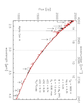
   Figure 1: Comparison between the ISO-SWS data of $\alpha$ Cen A (black) and the synthetic spectrum (red) with stellar parameters T_eff = 5830 K, $\log$ g = 4.35, M = 1.3 M_⊙, z = 0.25, $\xi_{t}$ = 1.0 $\rm{km\,s^{-1}}$, $\mathrm{{}^{12}C/^{13}C}$ = 89, $\varepsilon$(C) = 8.74, $\varepsilon$(N) = 8.26, $\varepsilon$(O) = 9.13 and $\theta_{d}$ = 8.80 mas. Some of the most prominent discrepancies between these two spectra are indicated by an arrow.

   The lack of reliable atomic data rendered the determination of the continuum of the hot stars very difficult. As a consequence, the uncertainty on the angular diameter is more pronounced. Therefore, Vega and Sirius have been used to check our findings, but they have not been studied into all detail. In order to deduce possible problems with calibration files, more trustworthy data as input for the theoretical models are needed.

2. The hydrogen lines are also conspicuous. For example, the synthetic hydrogen Pfund lines are almost always predicted as too strong for main-sequence stars, while they are predicted as too weak for the supergiant $\alpha$ Car (see Fig. 2, where the hydrogen lines are indicated by an arrow). This indicates a problem with the generation of the synthetic hydrogen lines, which is corroborated when the high-resolution ATMOS spectrum of the Sun is compared with its synthetic spectrum.

   

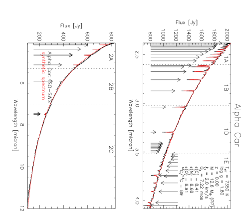
   Figure 2: Comparison between band 1 and band 2 of the ISO-SWS data of $\alpha$ Car (black) and the synthetic spectrum (red) with stellar parameters T_eff = 7350 K, $\log$ g = 1.80, M = 12.6 M_⊙, z = 0.00, $\xi_{t}$ = 2.0 $\rm{km\,s^{-1}}$, $\mathrm{{}^{12}C/^{13}C}$ = 89, $\varepsilon$(C) = 8.41, $\varepsilon$(N) = 8.68, $\varepsilon$(O) = 8.91 and $\theta_{d}$ = 7.22 mas. Hydrogen lines are indicated by an arrow.

3. Compared to the ISO-SWS data, the synthetic spectra of hot stars display a higher flux between the H5-9 and H5-8 hydrogen line (see Fig. 2). From other SWS observations available in the ISO data-archive, we could deduce that this ’pseudo-continuum’ starts arising for stars hotter than K0 ($\sim 4500$ K). Since such an effect was not seen for the cooler K and M giants, we could reduce the problem as having an atomic origin. A scrutiny on the hydrogen lines learns that the high-excitation Humphreys-lines (from H6-18 on) - and Pfund-lines - are always calculated as too weak. Moreover, the Humphreys ionization edge occurs at 3.2823 $\mu$m. Since the discrepancy does not appear above the limit (i.e. at shorter wavelengths) and is disappearing beyond the Brackett-$\alpha$ line, the conclusion is reached that the missing lines could well be the crowding of Humphreys hydrogen lines towards the series limit.

4. From 3.84 $\mu$m on, fringes at the end of band 1D affect the SWS spectrum of almost all stars in the sample.

5. A clear discrepancy is visible at the beginning of band 1A. For the hot stars, the H5-22 and H5-23 lines emerge in that part of the spectrum. An analogous discrepancy is also seen for the cool stars, though it is somewhat more difficult to recognize due to the presence of many CO features (Fig. 3). Being present in the continuum of both hot and cool stars, this discrepancy is attributed to problems with the RSRF. A broad-band correction was already applied at the short-wavelength edge of band 1A ([Vandenbussche1999]), but the problem seems not to be fully removed. At the band edges, the responsivity of a detector is always small. Since the data are divided by the RSRF, a small problem with the RSRF at these places may introduce a pronounced error at the band edge.

6. Memory effects make the calibration of band 2 for all the stars very difficult. These memory effects are more severe for the cool stars, since the CO and SiO absorptions cause a steep increase (decrease) in flux for the up (down) scan. The RSRFs for the sub-bands will therefore only be modeled well once there is a full-proof method to correct SWS data for detector memory effects.

3.2.2 Cool stars: G2-M2

1. The situation changes completely when going to the cool stars of the sample. While the spectrum of the hot stars is dominated by atomic-line features, molecules determine the spectral signature of the cool stars (Fig. 3). A few of the - problematic - atomic features (see Sect. 3.2.1) can still be identified in these cool stars. E.g. atomic spectral feature around 3.97 $\mu$m (Fig. 1) remains visible for the whole sample, even till $\alpha$ Cet.

   

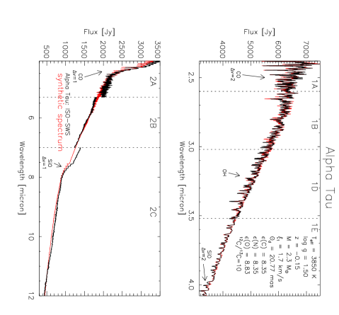
   Figure 3: Comparison between band 1 and band 2 of the ISO-SWS data of $\alpha$ Tau (black) and the synthetic spectrum (red) with stellar parameters T_eff = 3850 K, $\log$ g = 1.50, M = 2.3 M_⊙, z = -0.15, $\xi_{t}$ = 1.7 $\rm{km\,s^{-1}}$, $\mathrm{{}^{12}C/^{13}C}$ = 10, $\varepsilon$(C) = 8.35, $\varepsilon$(N) = 8.35, $\varepsilon$(O) = 8.83 and $\theta_{d}$ = 20.77 mas. The most important absorbers are indicated by an arrow.

2. One of the most prominent molecular features in band 1 is the first-overtone band of carbon monoxide (CO, $\Delta v=2$) around 2.4 $\mu$m. In these oxygen-rich stars, the total amount of carbon determines the strength of the CO band. This carbon abundance can be calculated in two ways:

   • the strong CO absorption causes a ’dip’ in the continuum till $\sim$ 2.8 $\mu$m, which may be used to determine $\varepsilon$(C);

   • the strength of the CO spectral features is directly related to $\varepsilon$(C).

   Computing a synthetic spectrum with the carbon abundance determined from this first criterion, results however in the (strongest) CO spectral features being always too strong compared to the ISO-SWS observation (2-4%). It has to be noted that this mismatch occurs in band 1A, where the standard deviation of the rebinned spectrum is larger than for the other sub-bands and that the error is within the quoted accuracy of ISO-SWS in band 1A ([Schaeidt et al.1996]). Nevertheless, it is alarming that this mismatch is not random, in the sense that the observed CO features are always weaker than the synthetic ones.

   The agreement between the high-resolution FTS spectrum and synthetic spectrum of $\alpha$ Boo is however extremely good. When scrutinizing carefully the first-overtone CO lines in the FTS spectrum, it was clear that all the ¹²CO 2-0 lines, and practically all the ¹²CO 3-1 lines, are predicted as too weak (by 1-2%)!

   Firstly, it has to be noted that the flux values in the wavelength region from 2.38 to 2.4 $\mu$m, where the CO 2-0 P18 and the CO 2-0 P21 are the main features, are unreliable due to problems with the RSRF of band 1A. Secondly, no correlation is found with the local minima and maxima in the RSRF of band 1A. Since the instrumental profile of an AOT01 is still not exactly known, the synthetic data were convolved with a gaussian with FWHM=$\lambda$/resolution. This incorrect gaussian instrumental profile introduces an error which will be most visible on the strongest lines. Together with too high a theoretical resolving power for an AOT01 speed-4 observation in band 1A ($\geq 1500$), these two instrumental effects may explain this discrepancy.

3. For both the high-resolution FTS and the medium-resolution SWS spectrum (Fig. 3), the strongest lines (OH 1-0 lines) are predicted as too weak, while the other lines match very well. Since the same effect occurs for these two different observations, it it plausible to assume that the origin of the problem is situated in the theoretical model or in the synthetic-spectrum computation. Wrong oscillator strengths for the OH lines could e.g. cause that kind of problems. Different OH line lists do however all show the same trend ([Decin2000]). Since a similar discrepancy was also noted for the low-excitation CO lines, a problem with the temperature distribution in the outermost layers of the stellar model is a very plausible explanation for this discrepancy.

4. The same remarks as for the hot stars, concerning the fringes and the memory effects, can be given.

So far, the origins of all the general discrepancies in band 1 for both hot and cool stars have been traced. With this in mind, the other stars of our sample have been studied carefully and the results are described in [*]DWE_decinthes.

4 IMPLICATION ON CALIBRATION AND MODELING

The results of this detailed comparison between observed ISO-SWS data and synthetic spectra have an impact both on the calibration of the ISO-SWS data and on the theoretical description of stellar atmospheres.

From the calibration point of view, a first conclusion is reached that the broad-band shape of the relative spectral response function is at the moment already quite accurate, although some improvements can be made at the beginning of band 1A and band 2. Also, a fringe pattern is recognized at the end of band 1D. Inaccurate beam profiles together with too high a resolving power may cause the strongest CO lines to be predicted as too strong. Since the same molecules are absorbing in band 1 and in band 2, these synthetic spectra are supposed to be also very accurate in band 2. These spectra will therefore be used to test the recently developed method for memory effect correction ([Kester2000]) and to rederive the relative spectral response function for band 2. The synthetic spectra of the standard sources of our sample are not only used to improve the flux calibration of the observations taken during the nominal phase, but they are also an excellent tool to characterize instabilities of the SWS spectrometers during the post-helium mission.

Concerning the modeling part, problems with the construction of the theoretical model and computing of the synthetic spectra are pointed out. The comparison between the high-resolution FTS spectrum of $\alpha$ Boo and the corresponding synthetic spectrum revealed that the low-excitation first-overtone CO lines and fundamental OH lines are predicted as too weak. This indicates a problematic temperature distribution in the outermost layers of the theoretical models. The upper photosphere is very difficult to model and is often computed from an extrapolation of the interior layers. The temperature distribution should now be disturbed in order to simulate a chromosphere, convection, a change in opacity, … Using these improved models, the change in abundance pattern resulting from the ISO-SWS data should be studied. The complex computation of the hydrogen lines, together with the inaccurate atomic oscillator strengths in the infrared rendered the computation of the synthetic spectra for hot stars difficult. In spite of the fact that the broadening parameters were thought to be taken into account properly, the ISO-SWS data displayed a notorious discrepancy for the Brackett, Pfund and Humphreys lines. People from the stellar-atmosphere-group in Uppsala are now scrutinizing this problem. The high-resolution ATMOS spectrum of the Sun and the SWS spectra of our standard sources indicated an insufficient knowledge of atomic oscillator strengths in the infrared. J. Sauval (Royal Observatory Belgium) is now trying to derive empirical oscillator strengths from the high-resolution ATMOS spectrum of the Sun.

Although we have mainly concentrated on the discrepancies between the ISO-SWS and synthetic spectra -s ince this was the main task of this research - we would like to emphasize the very good agreement between observed ISO-SWS data and theoretical spectra. The very small discrepancies still remnant in band 1 are at the 1-2% level for the giants, proving not only that the calibration of the (high-flux) sources has already reached a good level of accuracy, but also that the description of cool star atmospheres and molecular line lists is very accurate. The theoretical description of cool star atmospheres has lagged behind for a long time the description of hot star atmospheres, but, I think, that from now on, we may say that this is not anymore true!

References

- [\astronciteCohen et al.1992] Cohen M., Walker R.G., Witteborn F.C., 1992, AJ 104, 2030
- [\astronciteCohen et al.1995] Cohen M., Witteborn F.C., Walker R.G., Bregman J., Wooden D.H., 1995, AJ 110, 275
- [\astronciteCohen et al.1996b] Cohen M., Witteborn F.C., Carbon D.F., Davies J.K., Wooden D.H., Bregman J.D., 1996b, AJ 112, 2274
- [\astronciteDecin et al.1997] Decin L., Cohen M., Eriksson K., Gustafsson B., Huygen E., Morris P., Plez B., Sauval J., Vandenbussche B., Waelkens C., 1997, in ‘Proc. First ISO Workshop on Analytical Spectroscopy’, Heras, A.M., Leech, K., Trams, N.R., Perry, M. (eds.), ESA-SP 419, p. 185
- [\astronciteDecin et al.2000] Decin L., Waelkens C., Eriksson K., Gustafsson B., Plez B., Sauval A.J., Van Assche W., Vandenbussche B., 2000, A&A, submitted
- [\astronciteDecin2000] Decin L., 2000, in ‘Synthetic spectra of cool stars observed with the ISO Short-Wavelength Spectrometer: improving the models and the calibration of the instrument’, PhD. thesis, University of Leuven
- [\astronciteFarmer & Norton1989] Farmer C.B., Norton R.H., 1989, in ‘Atlas of the Infrared Spectrum of the Sun and the Earth Atmosphere from Space. Volume I, The Sun’, NASA Reference Publication 1224
- [\astronciteFeuchtgruber1998] Feuchtgruber H., 1998, in ‘Status of AOT01 AOT band order ratios and related data’, ISO-SWS online documentation
- [\astronciteGeller1989] Geller M., 1989, in ‘Atlas of the Infrared Spectrum of the Sun and the Earth Atmosphere from Space. Volume III. Key to Identification of Solar Features’, NASA Reference Publication 1224
- [\astronciteGustafsson et al.1975] Gustafsson B., Bell R.A., Eriksson K., Nordlund Å, 1975, A&A 42, 407
- [\astronciteHinkle et al.1995] Hinkle K., Wallace L., Livingston W., 1995, PASP 107, 1042
- [\astronciteKester2000] Kester D., 2000, in ‘ISO beyond the Peaks. The 2nd ISO workshop on analytical spectroscopy.’, A. Salama (eds.), SP-456, p. 93
- [\astronciteLorente1998] Lorente R., 1998, in ‘Spectral Resolution of SWS AOT 1’, ISO-SWS online documentation
- [\astronciteMonnier et al.1998] Monnier J.D., Geballe T.R., Danchi W.C., 1998, ApJ 502, 833
- [\astroncitePlez et al.1992] Plez B., Brett J.M., Nordlund Å, 1992, A&A 256, 551
- [\astroncitePlez et al.1993] Plez B., Smith. V.V., Lambert D.L., 1993, AJ 418, 812
- [\astroncitePourbaix et al.1999] Pourbaix D., Neuforge-Verheecke C., Noels A., 1999, A&A 344, 172
- [\astronciteSchaeidt et al.1996] Schaeidt S.G., Morris P.W., Salama A., et al., 1996, A&A 315, L55
- [\astronciteTsuji et al.1997] Tsuji T., Ohnaka K., Aoki W., Yamamura I., 1997, A&A 320, L1
- [\astronciteVandenbussche1999] Vandenbussche B., 1999, in ‘The ISO-SWS Relative Spectral Response Calibration’, ISO-SWS online documentation
- [\astronciteWitteborn et al.1999] Witteborn F.C., Cohen M., Bregman J.D., Wooden D.H., Heere K., Shirley E.L., 1999, AJ 117, 2552