Study of the Temporal Behavior of 4U 1728–34 as a Function of its Position in the Color-Color Diagram

Abstract

We study the timing properties of the bursting atoll source 4U 1728–34 as a function of its position in the X-ray color-color diagram. In the island part of the color-color diagram (corresponding to the hardest energy spectra) the power spectrum of 4U 1728–34 shows several features such as a band-limited noise component present up to a few tens of Hz, a low frequency quasi-periodic oscillation (LFQPO) at frequencies between 20 and 40 Hz, a peaked noise component around 100 Hz, and one or two QPOs at kHz frequencies. In addition to these, in the lower banana (corresponding to softer energy spectra) we also find a very low frequency noise (VLFN) component below $\sim 1$ Hz. In the upper banana (corresponding to the softest energy spectra) the power spectra are dominated by the VLFN, with a peaked noise component around 20 Hz. We find that the frequencies of the kHz QPOs are well correlated with the position in the X-ray color-color diagram. For the frequency of the LFQPO and the break frequency of the broad-band noise component the relation appears more complex. These frequencies both increase when the frequency of the upper kHz QPO increases from 400 to 900 Hz, but at this frequency a jump in the values of the parameters occurs. We interpret this jump in terms of the gradual appearance of a QPO at the position of the break at high inferred mass accretion rate, while the previous LFQPO disappears. Simultaneously, another kind of noise appears with a break frequency of $\sim 7$ Hz, similar to the NBO of Z sources. The 100 Hz peaked noise does not seem to correlate with the position of the source in the color-color diagram, but remains relatively constant in frequency. This component may be similar to several 100 Hz QPOs observed in black hole binaries.

1 Introduction

Low mass X-ray binaries (LMXBs) are usually characterized by weak magnetic fields. In these systems the accretion disk can reach regions close to the compact object, where the matter is subject to a strong gravitational field. This results in complex power spectra with characteristic frequencies, determined by the dynamical time scales close to the compact object, up to more than a thousand Hz. These timing structures can be used to probe the physics near the compact object, and timing is a key tool to perform such studies. Because several features are usually simultaneously present in the power spectra of LMXBs, we need to understand the entire timing structure in order to construct reliable theories for the different timing signals.

Power spectra of LMXBs show significant changes as a function of the source intensity and spectral hardness. Based on their spectral and temporal behavior, LMXBs can be divided into two classes, the so-called Z and atoll sources (Hasinger & van der Klis 1989), whose names are derived from the tracks they trace out in an X-ray color-color diagram. The Z sources are thought to have higher mass accretion rates and perhaps higher magnetic fields than the atoll sources. These two classes of sources show a temporal behavior that strongly depends on their position in the color-color diagram (Hasinger & van der Klis 1989). In particular, atoll sources can be found in the so-called island state, where the power spectrum is characterized by a strong band-limited noise component, called the high frequency noise (HFN), which extends up to tens of Hz in frequency, or in the banana state, where the power spectrum is dominated by a power-law noise below 1 Hz, usually called very low frequency noise (VLFN). It is thought that these states reflect different mass accretion rate, which increases from the island to the banana (see van der Klis 1995). In the island state the power spectrum usually shows other features, such as a low frequency quasi-periodic oscillation (hereafter LFQPO) between 20 and 40 Hz. This LFQPO, which may be similar to the horizontal branch oscillation (HBO) in Z sources, has been variously interpreted as due to the Lense-Thirring precession of material in the innermost disk region (Stella & Vietri 1998), to radial oscillations in the boundary layer between the neutron star surface and the accretion disk (Titarchuk & Osherovich 1999), or in terms of the magnetospheric beat frequency model (Alpar & Shaham 1985; Lamb et al. 1985; see also Psaltis et al. 1999a).

Observations with the Rossi X-Ray Timing Explorer (RXTE) have shown kilohertz quasi-periodic oscillations (kHz QPO) in the persistent emission of 20 LMXBs, with frequencies ranging from a few hundred Hz up to $1200-1300$ Hz (see van der Klis 2000 for a review). Usually two kHz peaks are simultaneously observed. The difference between the frequencies of the two simultaneous kHz QPOs is, in many cases, consistent with being constant. During type-I X-ray bursts in some atoll sources, nearly coherent oscillations were also detected at frequencies between 330 and 590 Hz, interpreted as the spin frequency of the neutron star (Strohmayer et al. 1996). In these cases the frequency separation between the two simultaneous kHz QPOs is similar to the frequency of the burst oscillations, or half that value (see Strohmayer, Swank, & Zhang 1998 for a review), suggesting a beat frequency mechanism as the origin of the kHz QPOs (Strohmayer et al. 1996; Miller, Lamb, & Psaltis 1998). However, the peak separation is sometimes significantly smaller than the frequency of the burst oscillations (Méndez, van der Klis, & van Paradijs 1998), and decreases as the frequency of the kHz QPOs increases (van der Klis et al. 1997; Méndez et al. 1998; Méndez & van der Klis 1999). Other models for the kHz QPOs are based on general relativistic periastron precession at the innermost disk boundary (Stella & Vietri 1999), or on relaxation oscillations that occur at the centrifugal barrier around the neutron star (Titarchuk, Lapidus, & Muslimov 1998).

The broad-band noise component, the LFQPO and the kHz QPOs seem to be correlated with each other and with the position of the source in the color-color diagram. The frequency of the LFQPO in Z-sources (i.e. the HBO) is correlated with the kHz QPO frequency (e.g. van der Klis et al. 1997; Wijnands et al. 1998; see also Psaltis, Belloni, & van der Klis 1999b, and references therein), as is the LFQPO in atoll sources (e.g. Stella & Vietri 1998; Ford & van der Klis 1998; van Straaten et al. 2000). The LFQPO in Z sources may differ from that in atoll sources, because they might be the second harmonic instead of the fundamental (cf. Jonker et al. 1998; Wijnands & van der Klis 1999). The break frequency of the broad-band noise component in atoll sources is also correlated with the kHz QPO frequency (Ford & van der Klis 1998; van Straaten et al. 2000; Reig et al. 2000) and such a component may also be present in Z-sources (Wijnands & van der Klis 1999). The correlation between the LFQPO and the kHz QPOs seems to be general, including also the $0.1-10$ Hz QPOs observed in black hole candidates (BHCs; Psaltis et al. 1999b). Another general correlation seems to exist between the frequency of the break of the broad-band noise component and the frequency of the LFQPO (Wijnands & van der Klis 1999). A detailed study of the kHz QPOs in several atoll sources revealed that there is a correlation between frequency and position in the color-color diagram (see e.g. Méndez & van der Klis 1999; Kaaret et al. 1999; Méndez 1999) or spectral shape (Ford et al. 1997a; Kaaret et al. 1998). These correlations suggest that all these properties depend on one parameter that could be the mass accretion rate (cf. Hasinger & van der Klis 1989). On the other hand, the relation between the frequency of the kHz QPOs and count rate is complex (Ford et al. 1997b; Yu et al. 1997; Zhang et al. 1998; Méndez 1999, and reference therein), suggesting that the X-ray flux is not a good indicator of the mass accretion rate.

One of the most interesting sources in this context is the bursting source 4U 1728–34. It belongs to the class of the atoll sources, and shows temporal variability on all time scales resulting in a complex power spectrum. It was observed with the EXOSAT satellite in the island state (Hasinger & van der Klis 1989), but a great deal of new information about this source has recently come from RXTE observations. 4U 1728–34 shows kHz QPOs (Strohmayer, Zhang, & Swank 1996) and burst oscillations at 363 Hz (Strohmayer et al. 1996). The peak separation between the kHz QPOs in this source is always smaller than 363 Hz, and decreases significantly at higher inferred accretion rates (Méndez & van der Klis 1999). Besides these high-frequency features, the power spectrum of this source also shows a broad-band noise component (with a break frequency around 10 Hz), a LFQPO (between 20 and 40 Hz; Strohmayer et al. 1996) and a bump around 100 Hz (Ford & van der Klis 1998). Both the centroid frequency of the LFQPO and the frequency of the break of the broad-band noise seem to be correlated with the frequency of the kHz QPOs (Ford & van der Klis 1998).

In this paper we present new results about the correlations between noise and QPOs in 4U 1728–34, obtained from a study of the temporal behavior of this source as a function of the position in the color-color diagram. For this analysis we used all the RXTE observations performed in 1996 and 1997, that are now publicly available (results from these data were already published by Strohmayer et al. 1996; Strohmayer, Zhang, & Swank 1997; Ford & van der Klis 1998; Méndez & van der Klis 1999). We find that, while the LFQPO frequency is correlated to both the kHz QPO and break frequencies at low inferred mass accretion rates, at higher accretion rate there is a jump in this correlation, probably because a new LFQPO appears at the position of the break, and another noise component appears in the power spectrum.

2 Observations and Analysis

We analyzed data of 4U 1728–34 from the public RXTE archive, using observations performed in 1996 between February 15 and March 1, 1996 on May 3, and 1997 between September 23 and October 1. The log of these observations is presented in Table 1.

From the instruments on board RXTE, we only used data from the Proportional Counter Array (PCA), selecting intervals for which the elevation angle of the source above the earth limb was greater than 10 degrees. We discarded those data ($\sim 2$% of the total) where 1 or 2 of the 5 PCA detectors were switched off. Several bursts occurred during these observations, but we excluded those intervals ($\sim 500$ s around each burst) from our analysis. We used the Standard 2 mode data (16 s time resolution) to produce light curves and the color-color diagram, and Event data (with a time resolution of 16 $\mu$s or 122 $\mu$s) to produce Fourier power spectra as described below.

We used the standard PCA background model 2.1b to extract background subtracted light curves binned at 16 s in the energy bands $2.0-3.5$, $3.5-6.4$, $6.4-9.7$, $9.7-16.0$ keV. We defined the soft color as the count rate ratio in the bands $3.5-6.4$ keV and $2.0-3.5$ keV, and the hard color as the ratio of count rates in the bands $9.7-16.0$ keV and $6.4-9.7$ keV, and produced a color-color diagram. Because the observations span two years, we took into account the gain changes of the PCA between epoch 1 (until 1996 March 21) and epoch 3 (from 1996 April 15 to 1999 March 22), as well as the additional continuous gain change that occurs within each epoch. As it can be seen in Table 1, 18 observations ($\sim 70\%$ of the observation time) took place in February-March 1996 during epoch 1, one observation occurred in May 1996 during epoch 3, and the remaining 9 observations occurred in September-October 1997, again during epoch 3. To correct the data for changes of the gain of the PCA, we proceeded as described in Kuulkers et al. (1994): we selected RXTE observations of Crab obtained close to the dates of our observations, and calculated X-ray colors for Crab. Between February 1996 and October 1997 the soft and hard colors of Crab increased by $\sim 16$ % and $\sim 5$ % respectively, and between May 1996 and October 1997 the same colors increased by $\sim 5$ % and $\sim 2$ %, respectively, so we applied these (multiplicative) corrections to the colors of 4U 1728–34. The resulting color-color diagram is shown in Figure 1. The reason to use Crab colors to estimate changes in the instrumental response is that the spectrum of Crab is supposed to be constant, and therefore changes in the colors of Crab are caused by changes in the instrumental response. However, the corrections calculated in this way do not take into account the difference in spectral shape between Crab and 4U 1728–34. We used spectral fits of 4U 1728–34 and the response matrices to test the magnitude of this effect. The correction factors obtained in this way are very similar to those calculated using Crab. They are $\sim 0.2$ % larger in soft color and $\sim 2$ % larger in hard color than the Crab-based correction factors, less than the statistical errors of the colors from each 16 s interval ($\sim 3$ % in both soft color and hard color). We preferred to use the Crab-based correction as it is independent of any model of either instrumental response or source spectrum.

To study the temporal variability of the source as a function of the position in the color-color diagram we divided this diagram into 19 intervals, as shown in Figure 1. The intervals were chosen in order to have a good number of intervals, and good statistics in each interval. For each interval we computed a power spectrum as follows: we divided the PCA light curve into segments 256 s long for which we calculated Fourier power spectra with no selection on energy, using a Nyquist frequency of 2048 Hz. Because every color point spans 16 s, each power spectrum corresponds to 16 color points. Due to the statistical uncertainties and to the motion of the source in the color-color diagram, a power spectrum could be spread over more than one interval (usually 2 to 3 intervals). For each interval, we averaged together all power spectra that fall in that interval for more than 30% of the time, weighing each of them by the fraction of the time it actually spent in the interval. We used 50% of the time in the upper banana (intervals 18 and 19), where the motion of the source in the color-color diagram is faster. This selection criterion allows some overlap between the nearest intervals. We checked that this overlap does not affect our results. In fact, the results we discuss in this paper do not significantly change if we use more restrictive selection criteria (without overlap between intervals), although QPO features are usually 10–20 % narrower in those cases. The power spectra, one for each interval selected in the color-color diagram, are indicated with numbers from 1 to 19 starting from the island state (upper right corner in the color-color diagram). Each interval contains from 10 to 134 power spectra. The high frequency part of each power spectrum ($1200-2048$ Hz, where neither noise nor QPOs are known to be present) was used to estimate the Poisson noise, which was subtracted before performing the spectral fitting.

In Figures 2a and 2b we show some representative power spectra (normalized as in Leahy 1983), corresponding to the intervals 4, 8, 10, 11, 12, 13, 14, and 19 of the color-color diagram of Figure 1. Power spectra 1–11 are typical of the island state of atoll sources, while 14 and 19 correspond to the lower and the upper banana respectively (see Hasinger & van der Klis 1989 for definitions). In spectra 1–11 we can distinguish several components: the HFN, with a break between 2 and 20 Hz, the LFQPO, between 10 and 40 Hz, a bump around 100 Hz, and one or two kHz QPOs. We used a broken power law, $P(\nu)\propto\nu^{-\alpha_{1,2}}$ where $\alpha_{1}$ is the power-law index below the break and $\alpha_{2}$ is the power-law index above the break, to describe the broad-band noise, and Lorentzians to describe the LFQPO, the 100 Hz peaked noise, and the kHz QPOs (when present). The characteristic frequencies of all these features are seen to increase from intervals 1 to 9. In intervals 10–13 a complex change is seen to occur in the power spectra. One way to describe this change is as follows: the break of the power law becomes sharper, and a bump is seen to occur on top of this break, which gradually turns into a QPO, pushing back the break to lower frequency. At the same time the original LFQPO, while still visible, weakens. We will discuss below how to describe this transition in terms of fits of the power spectra. In intervals 14 and higher, besides the previous components, we also see the VLFN, which we fitted using a power law, $P(\nu)\propto\nu^{-\alpha}$, with index $\alpha\sim 1.5-2.0$. The power spectrum of interval 19 appears much simpler than the others, consisting only of two noise components, namely the VLFN and the HFN. In this case the HFN appears to have a different shape from the one we observe in the island state, because it is peaked, i.e. the power law has a positive index before the break. Following Hasinger & van der Klis (1989), in this case we modeled the HFN using a power law with $\alpha<0$ plus an exponential cutoff ($\nu_{\rm cut}\sim 10$ Hz). For those intervals where the frequencies of the kHz QPOs were high enough that the kHz QPOs do not affect the parameters of the low frequency features and vice versa, we fitted the kHz QPOs in a limited frequency range (500–2048 Hz) where no other component was present. We then fitted the other components using the full frequency range and fixing the parameters of the kHz QPOs at the values obtained in the high frequency range. In particular, for interval 7 and for intervals 10 to 12 we did this with upper kHz QPO, and for intervals 13 to 17 we did it for both kHz QPOs. For the other intervals we fitted all the components (with all the parameters free) in the full frequency range.

The broad-band noise, the LFQPO, the 100 Hz peaked noise, and the kHz QPOs are detected in 17 of the 19 intervals in the color-color diagram (1 to 17), with the exception of the lower kHz peak that is absent in the first 9 intervals. The VLFN is detected in intervals 14 to 19. The broad-band noise is also detected (with a different shape) in intervals 18 and 19. In Table 2 we report the results of these fits and in Section 3 we discuss all these results in more detail.

In Figures 2a and 2b we also plot the best fit model and the corresponding residuals (in units of $\sigma$) for each power spectrum. For intervals 4 and 5 we obtain high reduced $\chi^{2}$: 4.5 and 4.1 (for 131 degrees of freedom), respectively. Looking at the residuals in Figure 2a, it is apparent that for these two intervals the main problem is the low frequency part of the power spectrum (below $\sim 3$ Hz, i.e. the frequency of the break), where the shape of the noise is curved, and is badly approximated by a power law (see also Section 2.2, where we try an alternative model for the noise component). Also, the abrupt change of the slope of the broken power law around the break frequency does not represent well the smooth change of the slope in the data there. Some residuals are also visible near the LFQPO (between 10 and 30 Hz) due to the shape of the QPO, that is sharper than a Lorentzian. For intervals 15 and 16 we obtain reduced $\chi^{2}$ of 2.3 and 2.6 (for 132 degrees of freedom), respectively. For these two intervals the largest residuals appear in the region of the kHz QPOs. In particular, the leading wing of the lower kHz QPO is not well fitted by the model. For all the other power spectra the reduced $\chi^{2}$ ranges from 1.3 to 2.0 (for $131-139$ degrees of freedom). These values are also rather large, but this is not surprising given the high statistics of the power spectra and their complexity. Nevertheless, for these other intervals the residuals in Figure 2a,b are usually within 3 $\sigma$. Most of the time the largest residuals occur in the low frequency part of the power spectrum (due to the curved shape of the noise), or around the break (due to the sharp shape of the model at the break frequency, compared to the smoother shape of the data there).

From all the above we conclude that the high values of $\chi^{2}$ we obtain in some cases are mainly due to the detailed shape of the noise component, which is not so well approximated by a broken power law. However, this does not affect strongly the parameters of the QPOs, where the residuals are usually flat, or the behavior of the break frequency of the broad-band noise component, even though a broken power law is sometimes an oversimplification of the complex shape of these power spectra. Under the applied model, our estimates of the statistical errors on the fit parameters, which use $\Delta\chi^{2}=1$, for a one-sigma single parameter error, therefore provide a good estimation of the total error for the QPO parameters. For the noise parameters systematic effects probably dominate. These will be addressed below.

The model described above gave the best fit for most of the intervals. It is also the most commonly used model in the literature, which allows us to compare our results to those obtained for other sources. However, we note that this model is not the only possible choice. For some intervals other models can fit the data equally well, and more complex models can fit better. This non-uniqueness of the model contributes systematic uncertainties to the parameters. In the next sections we try different models for the power spectra, and we discuss how the results can be affected by using different models. Our conclusion will be that, independently of the model chosen to describe the spectra, in intervals 10–12 a major change gradually occurs in the power spectra. In the model just described this change shows up as a jump in the frequency and rms amplitude of the HFN and the LFQPO (cf. Fig. 5) between intervals 12 and 13. Other models can place this jump earlier (between 9 and 10).

2.1 Presence of a second low frequency QPO

The results presented in the previous section were obtained by fitting the power spectra using always the same function. While this facilitates the study of the power spectral parameters as a function of the position in the color-color diagram, we must note that the power spectra of intervals 10 to 12 are more complex than the others, and extra components may be required to fit them properly (cf. Fig. 2). For those intervals, there is an excess of power, that can be fitted by an extra QPO, at about the break frequency of the broken power law that we used to fit the HFN. For instance, if we add this extra QPO to our fit function of interval 12, we get LFQPOs at $20.5\pm 0.3$ Hz and $46.5\pm 0.9$ Hz, while the break frequency of the HFN decreases to $6.6\pm 0.2$ Hz, compared to $\sim 20$ Hz when we only fit one LFQPO to the power spectrum. This extra LFQPO significantly improves the fit, as $\chi^{2}$ decreases from 192 for 131 degrees of freedom to 149 for 128 degrees of freedom (the F-test probability is $4\times 10^{-7}$). The addition of this extra QPO does not change the parameters of the other LFQPO, the 100 Hz peaked noise, and the kHz QPOs; the differences between the values of these parameters using these two different models are well within the errors. However, the inclusion of this extra LFQPO changes the parameters of the HFN. Both the break frequency we obtain for interval 12 using this model ($\sim 6.6$ Hz) and the frequency of the extra LFQPO ($\sim 20$ Hz) are in line with the results we obtain for interval 13. The change in the shape of the power spectra, that shows up in the model with only one LFQPO as a jump in the LFQPO frequency at interval 12–13 (to be discussed below), can be detected by the more complex model already in lower intervals. The results reported in Figures 2a and 2b and in Table 2 refer to the model with only one LFQPO.

2.2 Fitting the broad-band noise with a Lorentzian

For the first intervals, especially 4 and 5, the power spectra are not flat at low frequencies, and therefore not well fitted by a power law (cf. Fig. 2); we then get better fits using a Lorentzian instead of a broken power law. For interval 4, $\chi^{2}/d.o.f.=587/131$ using the broken power law, and $461/132$ using the Lorentzian, giving a statistically significant improvement (although the $\chi^{2}$ is still large). The Lorentzian fit becomes complicated, however, for intervals 10–12. The sharp break there (see Fig. 2) can not be fitted with the smoother Lorentzian. If we fit a Lorentzian anyway, this sharp edge appears as a QPO; two low frequency QPOs are now needed to fit these spectra. For interval 11, $\chi^{2}/d.o.f.=241/131$ for the broken power law and $182/129$ using the Lorentzian plus QPO for the broad-band noise, again a statistically significant improvement. Note that an extra LFQPO also improves the fit of intervals 10–12 when the broken power law is used to model the HFN (see Section 2.1). For the other intervals the fits are equally good whether we use a broken power law or a Lorentzian to represent the broad-band noise component.

The centroid frequency of the Lorentzian used to fit the broad-band noise goes from $0.51\pm 0.06$ Hz to $1.0\pm 0.1$ Hz for intervals 1 to 6, and it is around 3.2 ($\pm 0.3$) Hz for intervals 9 to 13. Its rms amplitude ranges from 15 to 20% up to interval 10; then it jumps down to 10% and continues decreasing to $\sim 3$%. This is the same jump that we see in the rms amplitude of the broken power law at interval 12–13 (Fig. 5): it occurs at interval 9–10 now because in intervals 10–12 the necessary extra QPO (centered near the break) absorbs some of the power. Comparing the half width at half maximum (HWHM) of the Lorentzian (plus the centroid frequency of the Lorentzian) and $\nu_{\rm break}$ in each interval, we see that there is a good correspondence between these two parameters up to interval 9, with the HWHM of the Lorentzian being a little bit larger than $\nu_{\rm break}$. In intervals 10 to 12 $\nu_{\rm break}$ increases (see Table 2b) while the HWHM of the Lorentzian is almost constant around 10 Hz. Again, this is due to the extra QPO at $\sim 20$ Hz. For intervals 13 to 17 both the HWHM of the Lorentzian and $\nu_{\rm break}$ are almost constant: $\nu_{\rm break}$ is $\sim 7$ Hz and the HWHM of the Lorentzian is $\sim 10-15$ Hz.

We conclude that the choice of either of these two models to fit the broad-band noise component does not affect the behavior of the parameters that we obtain, except for the width of the noise after interval 12. In fact, the parameters of all the other components that we obtain using a Lorentzian instead of the broken power law for the broad-band noise are consistent (usually within $1\sigma$; in a few cases the parameters of the LFQPO are within $3\sigma$) with the values already discussed, and show the same behavior when plotted against the frequency of the upper kHz QPO.

The addition of an extra LFQPO near 20 Hz in intervals 10–12, whether we use a Lorentzian for the HFN or a broken power law, modifies the width of the noise (break frequency or Lorentzian HWHM) and its rms amplitude, which jump to lower values ($\sim 7$ Hz and $\sim 7\%$, respectively). These results are in line with the parameters of the HFN and LFQPO in interval 13 and higher, indicating that a gradual change in the shape of the power spectra begins in intervals 10–12.

Finally, we also tried to fit these spectra using zero-centered Lorentzians for the noise and the bump at 100 Hz, as in Olive et al. (1998) for the source 1E 1724–3045. We did not obtain good fits, the principal reason being that the 100 Hz peaked noise can not be well fitted by a zero-centered Lorentzian for most of the intervals.

3 Results

We now describe the results from the fit with the model described in Section 2. We will note differences with the other fit function where appropriate in Section 4.

In Figure 3a we plot the frequencies of both kHz QPOs (upper panel) and their rms amplitudes (lower panel) as a function of the interval number in the color-color diagram. We also show the kHz QPO rms amplitudes as a function of the corresponding kHz QPO frequency in Figure 3b. While in the power spectra of intervals 10 to 17 we see both kHz QPOs, in the power spectra of intervals 1 to 9 (at low inferred mass accretion rate) we only see one of them, which in principle could be either the upper or the lower peak. However, when we plot the rms amplitude of the kHz QPOs vs. the position in the color-color diagram for all the intervals in which we detect kHz QPOs (Fig. 3a, lower panel), the rms amplitude of the single kHz QPO connects smoothly with the rms amplitude of the upper kHz QPO, whereas at the same time the rms amplitude of the lower kHz QPO is significantly lower. The same behavior is also visible in Figure 3b, where we plot the rms amplitude of each kHz QPO as a function of the corresponding frequency. We therefore conclude that when we only see one of the kHz QPO, it is always the upper peak (see also Ford & van der Klis 1998; Méndez & van der Klis 1999).

The frequencies of the kHz QPO range from $\sim 400$ to $\sim 1200$ Hz for the upper peak, and from $\sim 500$ to $\sim 900$ Hz for the lower peak. The frequencies of both QPOs are well correlated to the position of the source in the color-color diagram, although the frequency of the upper kHz QPO seems to jump from $\sim 500$ to $\sim 700$ Hz between intervals 6 and 7. This jump does not seem to be present in the plot of kHz QPO frequency versus position of the source in the color-color diagram (indicated with $S_{\rm a}$) shown in Méndez & van der Klis (1999; Fig. 4). However, this is because the jump is hidden by the intrinsic fluctuations of the kHz QPO frequency in the plot of Méndez & van der Klis (1999). If we average together points with similar values of $S_{\rm a}$ in their plot, we find that the average frequency of the kHz QPO remains more or less constant at $\sim 500$ Hz for $S_{\rm a}<1.4$, similar to what we observe for intervals 3–6, and then jumps to $\sim 700$ Hz for $S_{\rm a}\simeq 1.5$.

For both kHz QPOs the rms amplitude ranges from 3% to $\sim 12\%$, but while the rms amplitude of the upper peak generally decreases with frequency, the rms amplitude of the lower peak increases with frequency (except for the last point, which is significantly lower than the previous one). The width of the upper peak generally decreases with frequency. This implies higher values of the quality factor $Q=\nu/\Delta\nu$ (which ranges from $\sim 1.5$ to $\sim 9.5$), and therefore higher coherence of the signal, at higher frequency. For the lower peak no clear trend is evident. In this case Q ranges between 3.5 and 7.4 and is $\sim 15$ in the last interval in which the lower peak is detected. We note that in each interval we averaged many power spectra, and therefore the measured width of the kHz QPOs could be affected by changes in their centroid frequencies within the interval. In particular, we can estimate the effect of the frequency variations on the width of these features, considering the relation found for the frequency of the kHz QPOs versus interval number, and knowing that each power spectrum can be spread over at most three intervals. For interval numbers higher than 7, we find that the frequency of the kHz QPOs varies by $\sim 150$ Hz across 3 intervals. This is comparable with the measured widths of the kHz QPOs in interval 7 and higher where, therefore, the widths of the kHz QPOs are likely considerably affected by this broadening effect. For interval numbers lower than 7, the frequency of the kHz QPOs varies by $\sim 50$ Hz across 3 intervals. This is much smaller than the measured width of the kHz QPO (more than 200 Hz FWHM) in these intervals, indicating that the kHz QPOs may be intrinsically broader at low frequencies.

The 100 Hz peaked noise is a broad feature, with a FWHM that ranges from 100 to more than 200 Hz. Its frequency (Fig. 4, upper panel) seems to fluctuate around 130 Hz, without any clear correlation with the kHz QPO frequencies, although at higher values of the upper kHz QPO frequency ($\nu_{\rm high}>900$ Hz) it seems to increase with $\nu_{\rm high}$. Figure 4 (lower panel) shows the rms amplitude of the 100 Hz bump as a function of the frequency of the upper kHz QPO. For $\nu_{\rm high}<900$ Hz the rms amplitude of the 100 Hz bump stays constant at $\sim 10$%, and for $\nu_{\rm high}>900$ Hz it decreases to $\sim 4$%. It seems to be anti-correlated with the corresponding centroid frequency, at least at higher kHz QPO frequencies.

The broken power-law index below the break ($\alpha_{1}$) ranges from $-0.09\pm 0.04$ to $0.07\pm 0.02$, and the index above the break ($\alpha_{2}$) is almost constant around 1.5 (the typical error is 0.1), except for intervals 10 to 12 where it ranges between 2 and 2.5. This is because the shape of the power spectrum at the frequency of the break becomes sharp in these intervals, and probably another component begins to appear here (see Section 2.1). In Figure 5 (upper panel) we plot the break frequency of the broad-band noise component ($\nu_{\rm break}$) vs. the frequency of the upper kHz QPO. The break frequency increases from $\sim 2$ to $\sim 25$ Hz when $\nu_{\rm high}$ increases from $\sim 400$ Hz to 900 Hz. Beyond this frequency, $\nu_{\rm break}$ jumps down to 5 Hz and then remains constant around 7 Hz. The rms amplitude of the broad-band noise component (measured in the whole frequency range; Fig. 5, lower panel) generally decreases as the source moves in the color-color diagram from the island to the banana, as expected. In particular, it remains at $\sim 15\%$ up to $\nu_{\rm high}=800$ Hz where it starts decreasing; at $\nu_{\rm high}=900$ Hz, it jumps down to 5%, and continues decreasing down to $\sim 3$% as $\nu_{\rm high}$ increases.

Similar jumps at the same value of $\nu_{\rm high}=900$ Hz are also visible in the frequency and rms amplitude of the LFQPO (Fig. 5, upper and lower panel respectively). For $\nu_{\rm high}<900$ Hz the LFQPO frequency increases from 8 to 46 Hz as $\nu_{\rm high}$ increases. At $\nu_{\rm high}\sim 900$ Hz it jumps down to $\sim 20$ Hz, it then starts increasing again with $\nu_{\rm high}$, and finally seems to saturate. The rms amplitude of the LFQPO initially decreases from 15% to 3% as $\nu_{\rm high}$ increases up to 900 Hz; at that point the rms amplitude of the LFQPO jumps up to 10% and then decreases again from 10% to 5% as $\nu_{\rm high}$ increases.

Table 2b shows the parameters of the VLFN as a function of the interval number in the color-color diagram. The rms amplitude of the VLFN increases (from $\sim 1$% to $\sim 5\%$) with increasing inferred mass accretion rate, while the index of the power law is almost constant at 1.7. For intervals 18 and 19 we fitted the broad-band noise using a power law (with a positive index around 1.5) with an exponential cutoff at a frequency of $\sim 10$ Hz. The rms amplitude of this component is around 2%.

4 Discussion

The results illustrated in the previous section show that both the frequency and the rms amplitude of the kHz QPOs and X-ray colors are all well correlated with each other. It is thought that the position in the color-color diagram reflects different mass accretion rate (see e.g. Priedhorsky et al. 1986; Hasinger & van der Klis 1989; Hasinger et al. 1990; van der Klis 1994; Kaaret et al. 1998). Moreover, various models of the kHz QPOs associate their frequencies with the Keplerian frequency at the inner rim of the accretion disk (Miller et al. 1998; Titarchuk et al. 1998; Stella & Vietri 1999). The inner radius of the disk is thought to decrease with increasing mass accretion rate (Miller et al. 1998), suggesting that higher kHz QPO frequencies correspond to higher accretion rate. These considerations suggest that the mass accretion rate determines both the position of the source in the color-color diagram and the related timing behavior (cf. Hasinger & van der Klis 1989).

In the first 9 power spectra we only see one kHz QPO. In principle we can not say, in this case, if it is the lower or upper peak. Ford & van der Klis (1998) tentatively identified this QPO as the upper peak. This identification is in line with the result of Méndez & van der Klis (1999) that, in general, the single kHz QPO shows the same correlation with the inferred mass accretion rate as the upper peak. This identification is strengthened by our results presented here that there is a smooth trend of rms amplitude with QPO frequency if the single QPOs are identified with the upper of the two kHz QPOs (see Fig. 3b). This confirmation is important because the correlation of the LFQPO frequency with the frequency of the kHz QPOs lines up with that of other sources only if we make the identification as we do here (see e.g. Psaltis et al. 1999b).

We find that the parameters of the LFQPO and the broad-band noise are correlated with the frequency of the kHz QPOs in a complex way. As we can see in Figure 5, the frequencies of the LFQPO and of the break are correlated with the frequency of the upper kHz QPO up to $\nu_{\rm high}\sim 900$ Hz, which corresponds to interval 12, just before the appearance of the VLFN (see Table 2b). Beyond this frequency there is a jump in both the break and the LFQPO frequencies, confirming the trend already pointed out by Ford & van der Klis (1998). After the jump the frequency of the LFQPO seems to increase and then saturate at $\sim 40$ Hz while, except for the first point, $\nu_{\rm break}$ seems to be constant around 7 Hz. If for intervals 10–12 we use a model with an extra LFQPO (see Sections 2.1 and 2.2), the break of the HFN jumps to lower values, $\sim 6.6$ Hz. These values are similar to the break frequency measured in interval 13 and higher, indicating that the change in power spectral shape already begins in intervals 10–12 (corresponding to $\nu_{\rm high}\sim 850-900$ Hz). We also note that the frequency of the extra LFQPO ($\sim 20$ Hz) is similar to that of the LFQPO in intervals 13, suggesting that the LFQPO in intervals 13 and higher is the extra LFQPO present in 10–12, while the LFQPO at higher frequencies (present up to interval 12) disappears.

As mentioned in Section 2, looking carefully at the power spectra (Fig. 2), something is seen to happen starting at interval 10, namely an excess appears on top of the break at a frequency that is around half that of the LFQPO, while the LFQPO itself is fading as can be seen from its rms amplitude (Fig. 5, lower panel). In interval 12 two QPOs, one at 20 Hz (where we put the break frequency of the broken power law) and one at 46 Hz, could be present (see Sec. 2.1). So, the jump in the parameters of the LFQPO at $\nu_{\rm high}\sim 900$ Hz can be due to the fact that beyond this frequency we measure the parameters of what seems to be another LFQPO, which begins to appear at the frequency of the break already in intervals 10 to 12. At the same point, there is a jump in the parameters of the HFN (see Fig. 5 at $\nu_{\rm high}\sim 900$ Hz). This change can be identified in the power spectra: in interval 13 the HFN fits what appears to be another noise component characterized by a different behavior and a drastically lower break frequency ($\sim 7$ Hz). Some evidence of the emergence of this noise is already visible in the earlier power spectra (see Sec. 2.1). Jumps are also visible in the rms amplitudes of the noise component and of the LFQPO at $\nu_{\rm high}=900$ Hz (Fig. 5, lower panel). We note that at the same frequency similar variations (more gradual in this case) are also present in the rms amplitudes of the upper kHz QPO and the 100 Hz peaked noise, which both decrease from about 10% to $\sim 4$% (Fig. 3b and 4).

A possible interpretation of the behavior of the LFQPO and broken power-law break frequencies is that the noise component at low inferred accretion rates turns into a QPO at higher accretion rates, while what we call the LFQPO at low accretion rates gradually disappears at higher accretion rates. In Figure 5 (top) we can see that the centroid frequency of the LFQPO after the jump is in line with that of the break, as expected in this interpretation. A continuity is also visible between the rms amplitudes of the broken power law before the jump and the LFQPO after the jump (Fig. 5, bottom). We observe that the alternative models for intervals 10 to 12, containing an extra LFQPO, are also consistent with this interpretation, although the continuity between the rms amplitudes of the broken power law and the LFQPO is not observed in this case, because some of the power is absorbed by the extra LFQPO. After the jump the value of $\nu_{\rm break}$ seems to be constant around 7 Hz, which is in the same range of frequencies of the normal branch oscillations (NBOs) observed in the Z sources.

No QPO like the NBO are usually observed in atoll sources. For this reason these QPOs were associated with high accretion rates. Recently Wijnands et al. (1999) found that 4U 1820–30 shows a 7 Hz QPO at its highest mass accretion rate levels (see also Dotani et al. 1989). Going from the lower to the upper banana, in this source the broad-band noise seems to evolve into a broad peaked noise and then into a QPO around 7 Hz (Wijnands et al. 1999). This noise near 7 Hz seems quite similar to the noise after the jump shown by 4U 1728–34.

So, in 4U 1728–34 when mass accretion rate increases we see a noise component near 20 Hz turn into a QPO, while a new noise component appears at 7 Hz. This component at 7 Hz is similar to the one in 4U 1820–30, which in that source turns into a QPO when mass accretion rate increases further. We note that the noise we find after the jump in 4U 1728–34 seems to become peaked, i.e. before interval 13 the index $\alpha_{1}$ of the broken power law (below the break) is $\sim 0$, but after the jump at interval 13, $\alpha_{1}$ becomes negative (see Table 2b). A similar behavior was also observed in 4U 0614+09 (van Straaten et al. 2000).

In order to compare our results on 4U 1728–34 with similar results from other sources, we plotted in Figure 6 the frequencies of the break of the broad-band noise component (filled triangles) and of the LFQPO (open diamonds) on a logarithmic scale as a function of the lower kHz QPO frequency $\nu_{\rm low}$. For the first 9 intervals we calculated the frequency of the lower kHz QPO by subtracting an assumed constant peak separation of 363 Hz from the frequency of the upper kHz QPO. The frequency separation between the twin kHz QPOs in 4U 1728–34 is known to be constant for $\nu_{\rm low}$ between 600 and 800 Hz (Méndez & van der Klis 1999), and we are here extrapolating this result down to lower frequencies. We caution that it is unknown whether this peak separation remains constant down to the lowest kHz QPO frequencies. For instance, the relativistic precession model for the kHz QPOs (Stella & Vietri 1999) predicts that the peak separation should decrease at low frequencies (probably below $\nu_{\rm high}\sim 500-600$ Hz, depending on the mass of the compact object). This might explain the deviation of the points at the lowest frequencies from the observed correlations in Figure 6. A smaller peak separation would move these points towards higher values of $\nu_{\rm low}$, closer to the observed correlations.

Using the interpretation described above, we can distinguish three low frequency features, that are plotted in the diagram shown in Figure 6. The first one is the LFQPO at low accretion rate, that is correlated with the lower kHz QPO frequency (and therefore with the inferred mass accretion rate). As already known (Ford & van der Klis 1998), it follows a power law of index $\sim 0.95$ (the solid line drawn in Figure 6), the same as observed for the HBOs of the Z sources (Psaltis et al. 1999a,b. Note that line in Fig. 2 of Psaltis et al. 1999b has an index of 1.05). The second feature is the break of the broad-band noise which turns into a LFQPO at high accretion rate. This feature also seems to be correlated with the frequency of the lower kHz QPO. It follows a power law with index $\sim 1.5$ (the dashed line in Fig. 6). The third feature is the break frequency at high accretion rate, which we identify with the NBO of the Z sources and the 7 Hz QPO of 4U 1820–30.

Variabilities such as QPOs and broad noise components, have been observed in different kinds of accreting X-ray sources, like Z sources, atoll sources and BHCs. Recently some authors (Wijnands & van der Klis 1999; Psaltis et al. 1999b) have studied correlations between these components in order to understand if they could be explained by a single mechanism. Psaltis et al. (1999b) propose that two kinds of variability can be identified, one similar to the HBO of the Z sources and one similar to the kHz QPO, both in neutron star and in BHC systems, with different coherences and range of frequencies. The data used by Psaltis et al. (1999b) are also shown in Figure 6 (gray points). In the case of the BHC systems a $0.1-10$ Hz QPO is often accompanied by a $\sim 1-200$ Hz broad noise. Psaltis et al. (1999b) suggest to identify the first QPO with the HBO and the noise with the “kHz” QPO. When these two kinds of variabilities are plotted one against the other (PBK diagram; Psaltis et al. 1999b) a strong correlation appears that seems to extend the correlation observed for the Z sources over three orders of magnitude. In addition, the PBK diagram shows two more branches below this main branch, a second branch described by the BHCs XTE 1550–564 and GRO 1655–40, and the atoll source 4U 1608–52, and a third branch occupied by the NBO of the Z sources. If we compare our results on 4U 1728–34 with the plot shown in Psaltis et al. (1999b), we can see that our dashed line describing the break frequency at low mass accretion rate and the LFQPO at high mass accretion rate coincides with the second branch in PBK, and that $\nu_{\rm break}$ after the jump coincides with the third branch (see Fig. 6).

Another general correlation seems to exist between the frequencies of the LFQPO and the break for Z sources, atoll sources and BHCs, that is discussed in Wijnands & van der Klis (1999). These data are plotted in Figure 7 (gray points). In order to compare our results with this correlation (hereafter WK correlation) we plotted in Figure 7 the LFQPO frequency as function of $\nu_{\rm break}$ for 4U 1728–34 (filled triangles). We see that all the points before the jump follow the WK correlation, whereas the four points after the jump lie at $\nu_{\rm break}\sim 7$ Hz and $\nu_{\rm LFQPO}\sim 40$ Hz in Figure 7, slightly above the main relation, i.e. in the part of the diagram occupied by the Z sources. These correspond to higher accretion rates and follow a similar, but slightly shifted correlation, perhaps because the noise component is different in these sources (Wijnands & van der Klis 1999). The position of these points in the diagram also seems to suggest that, in 4U 1728–34 after the jump, another kind of variability is present, characterized by a different behavior. Note that with our proposed identification of $\nu_{\rm break}$ at low mass accretion rate with the second branch in the PBK diagram, we can now understand the WK correlation as the correlation between the main branch and the second branch in the PBK diagram. By plotting in the PBK diagram the break frequency vs. the lower kHz QPO frequency for other atoll sources this second branch will probably become further populated.

To summarize, we find that at low inferred mass accretion rate the frequency of the LFQPO and $\nu_{\rm break}$ are well correlated with the frequency of both kHz QPOs (and therefore with the inferred mass accretion rate). These frequencies describe two branches in the PBK diagram that are related through the WK relation. At high inferred mass accretion rate the previous LFQPO disappears and the broad-band noise changes into a QPO with a centroid frequency that corresponds to the break frequency of the previous noise. In the PBK diagram this new LFQPO falls in the same branch as the break frequency before the change. A new broad-band noise appears at these high accretion rates, characterized by a break frequency around 7 Hz. This could correspond to the NBO observed in Z sources, and also in the atoll source 4U 1820–30, at high accretion rate. All these results seem to indicate that there is a tight relation between noise and QPOs. In fact there is evidence that noise could change into a QPO and vice versa. Moreover, their characteristic frequencies show a precise dependence on inferred accretion rate, which shows up as the three branches in the PBK diagram.

The jump in the frequency of the LFQPO can be understood in the framework of the magnetospheric beat frequency model assuming that the neutron star magnetic field is approximately but not exactly dipolar (e.g., a dipole offset from the center of the star). In this case, at lower accretion rates, when the magnetospheric radius is far from the neutron star, the gas in the disk feels primarily the dipolar field. This is symmetric, and the LFQPO frequency will be double the difference between the orbital frequency at the magnetospheric radius and the spin frequency. At higher accretion rates, when the magnetospheric radius moves closer to the stellar surface, the gas in the disk feels primarily the offset, asymmetric field and the beat frequency will be the difference between the orbital and the spin frequency.

However, a phenomenology where LFQPO can mutate into broad-band noise and vice versa is probably more easily accommodated by models in which the LFQPO arises due to disk fluctuations (e.g., Titarchuk & Osherovich 1999; Psaltis & Norman 1999) than by those in which they are produced by orbital motion at the magnetospheric radius (Psaltis et al. 1999a) or Lense-Thirring precession of free-orbiting self-luminous blobs at the inner disk whose orbital radius is the upper kHz QPO frequency (Stella & Vietri 1998), particularly if the kHz QPO maintain a high Q while at the same time the LFQPO turns into broad noise. We point out, however, that disk fluctuation models do appear to be able to provide variability at or near the frequencies predicted by such orbital models (Alpar & Yilmaz 1997; Psaltis & Norman 2000).

The 100 Hz broad bump seems not to follow these general correlations, but instead to remain relatively constant in frequency at low inferred mass accretion rate. At higher accretion rate the frequency increases, while the rms amplitude decreases. We note that this component might be similar to the QPOs between 67 and 300 Hz that have been found in several BHCs (Morgan, Remillard, & Greiner 1997; Remillard et al. 1999a; Remillard et al. 1999b; Homan et al. 2000). A similar QPO near 100 Hz is also seen in the atoll source 4U 0614+09 (van Straaten et al. 2000).

Table 1: RXTE observations of 4U 1728–34 used in our analysis. The count rate corresponds to 5 PCA units and is corrected for background.

Start Time	Total Time	Averaged Rate
(UTC)	(ksec)	(c/s)
15/02/’96 11:51	25	1863
15/02/’96 18:59	18	1948
16/02/’96 00:03	20	2060
16/02/’96 06:26	15	2172
16/02/’96 15:49	21	2160
16/02/’96 22:15	10	2199
18/02/’96 11:10	25	1609
18/02/’96 19:15	15	1516
22/02/’96 11:33	25	996
22/02/’96 19:12	15	997
23/02/’96 21:16	30	978
24/02/’96 05:17	5	1090
24/02/’96 17:51	25	1022
25/02/’96 01:15	12	1034
25/02/’96 20:51	25	1080
26/02/’96 04:02	15	1093
29/02/’96 23:12	0.8	1200
01/03/’96 00:13	20	1193
03/05/’96 14:03	2.1	1126
23/09/’97 23:50	1.2	2190
24/09/’97 09:14	25	2582
24/09/’97 17:15	4	2422
26/09/’97 12:30	25	1775
27/09/’97 09:19	25	1506
30/09/’97 04:34	15	1799
30/09/’97 10:57	8	1793
01/10/’97 06:09	25	1659
01/10/’97 14:10	3.5	1683

Table 2a: Fitted parameters of the kHz QPOs and the peaked noise at 100 Hz.

		Upper kHz QPO			Lower kHz QPO			100 Hz peaked noise
Interval	Rate	Frequency	FWHM	rms	Frequency	FWHM	rms	Frequency	FWHM	rms
Number	(c/s)	(Hz)	(Hz)	(%)	(Hz)	(Hz)	(%)	(Hz)	(Hz)	(%)
1	1315	387$\pm$18	230$\pm$73	9.6$\pm$2.1	-	-	-	64$\pm$37	350$\pm$110	16.3$\pm$3.1
2	1285	397$\pm$14	270$\pm$37	10.57$\pm$0.97	-	-	-	110$\pm$20	269$\pm$61	12.5$\pm$2.0
3	1209	466$\pm$21	295$\pm$52	12.0$\pm$1.2	-	-	-	163$\pm$15	205$\pm$61	10.4$\pm$1.6
4	1156	497.8$\pm$5.3	282$\pm$17	12.80$\pm$0.34	-	-	-	154.7$\pm$3.6	164$\pm$14	10.51$\pm$0.44
5	1155	498.7$\pm$5.9	287$\pm$18	12.44$\pm$0.35	-	-	-	151.5$\pm$4.0	183$\pm$16	10.79$\pm$0.46
6	1151	517.3$\pm$8.1	219$\pm$26	11.10$\pm$0.59	-	-	-	169.8$\pm$9.6	220$\pm$33	11.22$\pm$0.86
7	1375	694.5$\pm$9.3	206$\pm$33	13.31$\pm$0.68	-	-	-	153$\pm$11	118$\pm$47	8.9$\pm$1.8
8	1510	729.0$\pm$3.5	162.6$\pm$8.5	11.77$\pm$0.26	-	-	-	106$\pm$21	211$\pm$38	10.7$\pm$1.8
9	1605	789.6$\pm$2.5	143.4$\pm$5.7	11.52$\pm$0.19	-	-	-	72$\pm$24	239$\pm$27	12.5$\pm$2.0
10	1722	846.9$\pm$2.0	133.0$\pm$6.0	10.93$\pm$0.19	511$\pm$17	98$\pm$48	3.12$\pm$0.54	94.6$\pm$9.0	190$\pm$15	12.14$\pm$0.90
11	1739	872.9$\pm$1.6	131.1$\pm$4.3	10.54$\pm$0.13	559$\pm$11	88$\pm$32	2.98$\pm$0.35	91.4$\pm$5.4	167.5$\pm$9.2	11.39$\pm$0.54
12	1732	905.2$\pm$2.6	134.5$\pm$7.4	10.12$\pm$0.22	599$\pm$14	139$\pm$30	4.60$\pm$0.39	103.9$\pm$5.4	149$\pm$12	10.76$\pm$0.57
13	1865	948.8$\pm$3.8	158$\pm$12	8.30$\pm$0.26	673$\pm$10	191$\pm$33	5.82$\pm$0.41	121.9$\pm$3.0	98$\pm$10	6.86$\pm$0.33
14	1871	1054.7$\pm$8.7	166$\pm$27	5.62$\pm$0.33	750.9$\pm$3.7	121.8$\pm$9.3	7.04$\pm$0.22	142.1$\pm$5.4	87$\pm$14	4.54$\pm$0.34
15	1907	1105.8$\pm$6.8	148$\pm$19	4.79$\pm$0.22	773.0$\pm$1.8	103.8$\pm$5.1	7.16$\pm$0.13	159.1$\pm$5.4	94$\pm$16	3.85$\pm$0.29
16	1861	1129$\pm$13	117$\pm$22	3.38$\pm$0.27	816.0$\pm$4.0	166.0$\pm$6.6	7.82$\pm$0.13	146.5$\pm$8.7	102$\pm$16	3.68$\pm$0.27
17	1939	1158$\pm$18	129$\pm$56	3.68$\pm$0.54	876.1$\pm$2.6	59.5$\pm$7.2	5.59$\pm$0.24	210$\pm$32	180$\pm$74	3.96$\pm$0.74
18	2500	-	-	-	-	-	-	-	-	-
19	2600	-	-	-	-	-	-	-	-	-

Table 2b: Fitted parameters of the broad-band noise, the low-frequency QPO and the very low frequency noise.

	HFN				LFQPO			VLFN
Interval	$\alpha_{1}$	break or cutoff	$\alpha_{2}$	rms	Frequency	FWHM	rms	$\alpha$	rms	$\chi^{2}(d.o.f.)$
Number	$(\times 10^{-2})$	(Hz)		(%)	(Hz)	(Hz)	(%)		(%)
1	$-1.5$$\pm$1.5	1.392$\pm$0.038	1.55$\pm$0.14	13.7$\pm$1.1	8.08$\pm$0.43	15.43$\pm$0.79	17.00$\pm$0.95	-	-	241 (131)
2	$-2.4$$\pm$1.2	1.364$\pm$0.055	1.35$\pm$0.11	15.4$\pm$1.7	8.63$\pm$0.30	15.19$\pm$0.74	15.93$\pm$0.85	-	-	273 (131)
3	2.6$\pm$1.1	1.891$\pm$0.039	1.348$\pm$0.061	14.74$\pm$0.90	9.04$\pm$0.58	24.10$\pm$0.95	17.15$\pm$0.78	-	-	270 (131)
4	2.91$\pm$0.57	2.804$\pm$0.031	1.543$\pm$0.058	14.07$\pm$0.50	13.37$\pm$0.36	26.01$\pm$0.69	16.02$\pm$0.46	-	-	587 (131)
5	3.10$\pm$0.55	2.817$\pm$0.029	1.467$\pm$0.043	14.63$\pm$0.46	13.84$\pm$0.32	25.88$\pm$0.65	15.48$\pm$0.40	-	-	538 (131)
6	1.2$\pm$1.0	2.978$\pm$0.058	1.422$\pm$0.082	15.00$\pm$0.90	15.10$\pm$0.62	27.1$\pm$1.4	15.02$\pm$0.75	-	-	267 (131)
7	6.8$\pm$1.7	8.94$\pm$0.58	1.314$\pm$0.090	18.4$\pm$1.3	26.17$\pm$0.85	12.8$\pm$3.9	6.2$\pm$1.0	-	-	219 (134)
8	4.77$\pm$0.87	10.39$\pm$0.21	1.385$\pm$0.089	15.8$\pm$1.0	28.99$\pm$0.57	20.0$\pm$2.7	7.04$\pm$0.59	-	-	282 (131)
9	2.27$\pm$0.77	13.90$\pm$0.22	1.511$\pm$0.098	14.94$\pm$0.92	35.58$\pm$0.46	12.0$\pm$1.6	4.44$\pm$0.33	-	-	254 (131)
10	2.21$\pm$0.77	19.05$\pm$0.29	2.05$\pm$0.21	12.23$\pm$0.57	41.63$\pm$0.80	16.3$\pm$2.7	4.20$\pm$0.51	-	-	275 (131)
11	1.54$\pm$0.63	21.08$\pm$0.22	2.22$\pm$0.16	11.62$\pm$0.35	45.16$\pm$0.75	12.7$\pm$2.5	3.16$\pm$0.25	-	-	241 (131)
12	1.78$\pm$0.93	23.63$\pm$0.41	2.62$\pm$0.31	10.86$\pm$0.42	46.52$\pm$0.93	13.5$\pm$3.9	3.22$\pm$0.60	-	-	192 (131)
13	$-8.2$$\pm$4.3	5.06$\pm$0.32	1.42$\pm$0.18	5.26$\pm$0.67	22.22$\pm$0.76	39.2$\pm$2.0	10.61$\pm$0.38	-	-	181 (134)
14	$-9.2$$\pm$4.7	6.60$\pm$0.40	1.29$\pm$0.10	5.56$\pm$0.45	36.99$\pm$0.60	28.3$\pm$2.0	6.54$\pm$0.24	1.64$\pm$0.19	1.05$\pm$0.12	203 (132)
15	$-2.4$$\pm$3.9	6.91$\pm$0.39	1.299$\pm$0.094	4.72$\pm$0.32	40.44$\pm$0.33	22.0$\pm$1.1	5.55$\pm$0.13	1.68$\pm$0.11	1.284$\pm$0.091	305 (132)
16	$-4.9$$\pm$5.5	7.06$\pm$0.61	1.34$\pm$0.11	4.03$\pm$0.29	41.77$\pm$0.36	21.3$\pm$1.3	5.16$\pm$0.14	1.784$\pm$0.080	1.82$\pm$0.11	348 (132)
17	$-9$$\pm$19	6.5$\pm$1.3	1.31$\pm$0.57	3.11$\pm$0.97	41.0$\pm$1.1	25.8$\pm$3.9	4.80$\pm$0.36	1.718$\pm$0.087	3.39$\pm$0.31	191 (132)
18	-	14.6$\pm$4.4	$-1.38$$\pm$0.51	2.60$\pm$0.16	-	-	-	1.712$\pm$0.033	5.66$\pm$0.26	179 (139)
19	-	9.38$\pm$3.0	$-1.54$$\pm$0.61	2.16$\pm$0.16	-	-	-	1.602$\pm$0.028	4.73$\pm$0.17	184 (139)

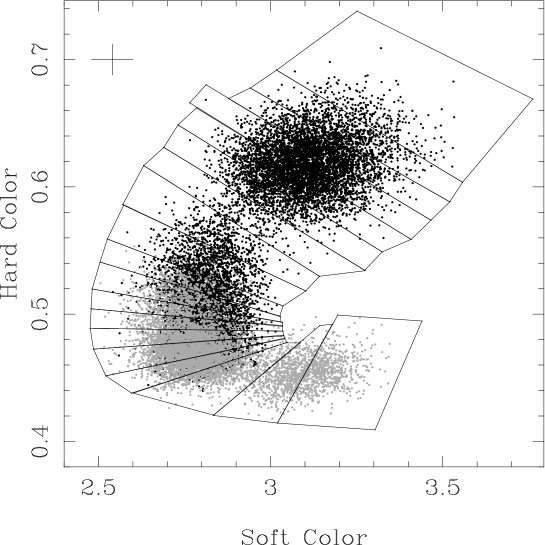
Figure 1: Color-color diagram of 4U 1728–34. The soft and hard colors are defined as the ratio of the count rate in the bands $3.5-6.4$ keV/$2.0-3.5$ keV, and $9.7-16$ keV/$6.4-9.7$ keV, respectively. Each point represents 16 s of data. Black points represent epoch 1 data (until 1996 March 21), and gray points represent epoch 3 data (from 1996 April 15 to 1999 March 22). A typical error bar is shown at the top left corner of the diagram. The boxes in the color-color diagram indicate the intervals we used to select the power spectra.

Fig. 2a.    Representative Leahy normalized power spectra of 4U 1728–34 corresponding to different intervals in the color-color diagram of Figure 1. Interval numbers are indicated. For each interval the power spectrum and the best fit model (including always at most one LFQPO, see text) are shown in the upper panel, and the corresponding residuals (in units of $\sigma$) are shown in the lower panel.

Fig. 2b.    Same as Figure 2a.

Fig. 3a.    Frequencies (upper panel) and rms amplitudes (lower panel) of the kHz QPOs as a function of the interval number in the color-color diagram. Different symbols are used for the lower peak (filled triangles) and the upper peak (open diamonds). Open squares represent intervals where we only detected one of the kHz QPOs.

Fig. 3b.    Rms amplitudes of the kHz QPOs as a function of the corresponding kHz QPO frequency. Symbols are as described in Figure 3a.

Fig. 4.    Frequency (upper panel) and rms amplitude (lower panel) of the 100 Hz peaked noise as a function of the frequency of the upper kHz QPO.

Fig. 5.    Parameters of the HFN and LFQPO as a function of the frequency of the upper kHz QPO. Different symbols are used for the HFN (filled triangles) and LFQPO (open diamonds). Upper panel: break frequency of the HFN and centroid frequency of the LFQPO. Lower panel: rms amplitudes of the HFN (calculated from 0 Hz to infinity) and of the LFQPO.

Fig. 6.    Frequencies of the LFQPO (open diamonds) and of the break (filled triangles) as a function of the frequency of the lower kHz QPO, $\nu_{\rm low}$. In the first 9 intervals $\nu_{\rm low}$ is calculated by subtracting the assumed constant peak separation of 363 Hz from the frequency of the upper kHz QPO that has been detected. For comparison, data for several LMXBs (including Z sources, atoll sources and black hole candidates, from Psaltis et al. 1999b) are also shown (gray points). Correlations between these frequencies are visible: the solid line is a power law of index 0.95 (Psaltis et al. 1999b) and the dashed line is a power law of index 1.5.

Fig. 7.    Centroid frequency of the LFQPO as a function of the break frequency of the HFN (filled triangles). For comparison, data for several LMXBs (including Z sources, atoll sources and black hole candidates, from Wijnands & van der Klis 1999) are also shown (gray points). These frequencies follow the WK correlation, except for four points at $\nu_{\rm break}\sim 7$ Hz and $\nu_{\rm LFQPO}\sim 40$ Hz, corresponding to frequencies of the upper kHz QPO higher than 900 Hz.