Radio Halos of Galaxy Clusters from Hadronic Secondary Electron Injection in Realistic Magnetic Field Configurations

Abstract

We investigate the possibility that radio halos of clusters of galaxies are caused by synchrotron emission of cosmic ray electrons (CRe), which were produced by cosmic ray protons (CRp) interacting hadronically with the intra-cluster medium (ICM) protons. We perform cosmological magneto-hydrodynamics (MHD) simulations to obtain a sample of ten magnetized galaxy clusters. They provide realistic models of the gas and magnetic field distribution, needed to predict the CRe production rates, their cooling, and their synchrotron emissivity. We assume a CRp population within the ICM with an energy density which has a constant ratio to thermal energy density. This ratio is adjusted in such a way that one of the simulated clusters reproduces the radio luminosity of the radio halo of the Coma cluster of galaxies. Our model exhibits the observed low degree of radio polarization and has a similar radial emission profile as the Coma cluster. We provide estimates for the expected gamma ray and neutrino flux. The necessary CRp/thermal energy ratio is 4 … 14 % ${(E_{\rm p,min}/{\rm GeV})}^{-0.375}$ (for the range of magnetic field strengths suggested by Faraday measurements), where $E_{\rm p,min}$ is the lower kinetic energy cutoff of the CRp with spectral index $\alpha_{\rm p}\approx 2.375$. Assuming this ratio to be the same in the whole set of simulated clusters a $T_{\mathrm{x}}-L_{\nu}$ relation is predicted which follows the observed relation well.

1 Introduction

Some clusters of galaxies contain large, Mpc-sized regions of diffuse radio emission, the so called cluster radio halos and cluster radio relics. Although known for decades, these sources receive increasing attention due to the improved detection sensitivities and their important theoretical implications for the non-thermal content of the ICM. For reviews see Valtaoja Valtaoja (1984), Jaffe Jaffe (1992), Feretti & Giovannini Feretti & Giovannini (1996), Feretti Feretti (1999), Enßlin Enßlin (1999b), and Giovannini et al. Giovannini et al. (1999).

Whereas the cluster relic sources are nowadays widely believed to trace the presence of large shock waves in the ICM Enßlin et al. (1998); Roettiger et al. (1999); Enßlin & Krishna (2000) the origin of radio halos is less clear. The lifetime of the radio emitting CRe is much shorter than any reasonable transport time over cluster scales. This means that the CRe need to be continuously re-energized, or freshly injected on a cluster-wide scale. The latter would happen if the CRe result from the decay of charged pions produced in hadronic interaction of energetic CRp distributed throughout the cluster volume Dennison (1980); Vestrand (1982); Valtaoja (1984); Schlickeiser et al. (1987); Blasi & Colafrancesco (1999). The CRp have lifetimes in the IGM of the order of a Hubble time Berezinsky et al. (1997); Enßlin et al. (1997), giving them enough time to diffuse away from their source and to maintain a cluster wide distribution.

It is the purpose of this work to demonstrate that a simple model for hadronic electron injection in a realistic magnetic field configuration leads to radio halos which reproduce several observations: the profile of the radialy decreasing radio emission, the low radio polarization, the radio to X-ray surface brightness correlation, and the cluster radio halo luminosity-temperature relation. We do not attempt to reproduce all observational information on cluster radio halos. For example the observed spatial spectral index variations of individual clusters Giovannini et al. (1993); Deiss et al. (1997) are not reproduced by the presented model. It is our goal to investigate the observational consequences of a conceptually simple model. Sophisticated modifications, which fine-tune the model to the data, are principally possible. But first an understanding of idealized models is most helpful. The assumptions of our model are:

1. CRe are secondary particles of hadronic interactions of CRp with the background protons of the ICM. The origin of the CRp is not specified here, but a likely explanation is particle acceleration in shock waves of cluster merger events and in accretion shocks of the clusters Colafrancesco & Blasi (1998). ICM CRp might also migrate from radio plasma of radio galaxies into the ICM Valtaoja (1984); Enßlin et al. (1997); Enßlin (1999a); Blasi & Colafrancesco (1999) or result from supernova driven galactic winds Volk et al. (1996).

2. The energy density in CRp is assumed to be proportional to the energy density of the thermal ICM gas. This is reasonable if the thermal gas and the CRp were energized in the same shock waves of cluster mergers, since a constant fraction of energy dissipated in the shock should go into the CRp population. Previous work ignored the spatial profiles Dennison (1980); Vestrand (1982) or assumed one single central point source from which the CRp diffused away, resulting in a centrally very peaked CRp profile Blasi & Colafrancesco (1999).

3. The CRp spectral index is independent of position or cluster and therefore the radio spectral index is constant in this model. Although this is certainly an oversimplification since e.g. the radio halo of the Coma cluster does show spectral index variations, it allows to predict radio halo statistics.

4. No significant re-acceleration or particle diffusion of the CRe is occurring.

5. The radio spectrum is assumed to be quasi-stationary, since the electron cooling time is short and a stationary CRe population is rapidly established. The spectrum of this population results from the shape of the proton spectrum, which is assumed to be a single power-law, and the synchrotron and inverse Compton cooling. Hence electron and radio spectra are also power laws.

6. The magnetic field configuration results from amplification of pre-cluster seed fields as simulated by Dolag et al. Dolag et al. (1999). We therefore investigate very inhomogeneously magnetised clusters. Although the importance of realistic field configurations for the appearence of radio halos was stressed by Tribble Tribble (1991), even recent work on halos of hadronic origin assumed spatially constant field strength.

2 MHD Cluster Formation Simulation

Figure 1: The radial profile of the magnetic field strength of the simulated clusters is shown in units of the virial radius $R_{200}$. The solid line represents the field strength in the cluster Sim.9. The thick dotted line is the profile averaged over all ten simulations, the thin dotted lines are the minimum and maximum values found in the different simulations.

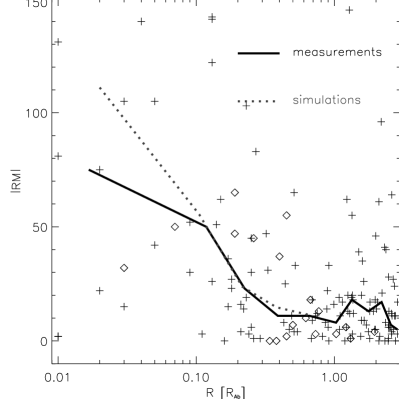
Figure 2: Comparison of synthetic Faraday-rotation measurements with a sample of measurements in Abell clusters. The absolute values of Faraday rotation measurements Kim et al. (1991) vs. radius in units of the Abell radius are shown. Obviously, the dispersion increases towards the cluster center. The solid curves mark the median of the measurements, the dotted curve is the median obtained from the simulated cluster sample. Some measurements have Faraday measurements which are outside the region shown (marked by the arrows on top of the plotting region). The median was chosen because it is not influenced by such values. The flattening of the observations towards the cluster center seems to be an artefact in the data. A comparison with newer data Clarke et al. (1999, 2000) shows that the inner-most bin is also perfectly in agreement with the simulations.

We used the cosmological MHD code described in Dolag et al. Dolag et al. (1999) to simulate the formation of magnetised galaxy clusters from an initial density perturbation field. The evolution of the magnetic field is followed from an initial seed field. This field is amplified by the compression during the cluster collapse. Merger events and sheer flows, which are very common in the cosmological environment of large-scale structure, lead to Kelvin-Helmholtz instabilities. They further increase the field strength by a large factor. In order to reproduce the present $\mu$G fields an initial nG field strength is required.

2.1 GrapeSPH

The code combines the merely gravitational interaction of a dark-matter component with the hydrodynamics of a gaseous component. The gravitational interaction of the particles is evaluated on GRAPE boards, while the gas dynamics is computed in the SPH approximation. It was also supplemented with the magneto-hydrodynamic equations to trace the evolution of the magnetic fields which are frozen into the motion of the gas because of its assumed ideal electric conductivity. The back-reaction of the magnetic field on the gas is included. Extensive tests of the code were successfully performed and described in the previous paper. $\@vec{\nabla}\cdot\@vec{B}$ is always negligible compared to the magnetic field divided by a typical length scale. The code also assumes the ICM to be an ideal gas with an adiabatic index of $\gamma=5/3$ and neglects cooling. The surroundings of the clusters are dynamically important because of tidal influences and the details of the merger history. In order to account for this the cluster simulation volumes are surrounded by a layer of boundary SPH particles in order to represent accurately the sources of the tidal fields in the cluster neighborhood. For details of the code, the models and the obtained magnetic field structure see Dolag et al. (1999; in preparation).

2.2 Initial conditions

For an accurate calculation of the synchrotron emission the resolution of the magnetic field is crucial. We therefore perform simulations in a CDM Einstein-de-Sitter cosmology ($\Omega_{\mathrm{m}}^{0}=1.0$, $\Omega_{\Lambda}^{0}=0$, $H_{0}=50\,{\rm km\,s^{-1}\,Mpc^{-1}}$), with twice the mass resolution of the simulation described in Dolag (1999). We simulate a set of ten different realisations which result in clusters of different final masses and different dynamical states at redshift $z=0$.

As shown in Dolag 1999, the initial field structure is irrelevant because the final field structure is mostly determined by the dynamics of the cluster collapse. The initial field strengths in this simulations where chosen so that the final field strength reproduces the observed Faraday rotation data collected by Kim et al. Kim et al. (1991). The central values of the ten clusters vary between $0.5\mu$G and $2\mu$G, whereas Sim.9 reaches values of $\approx 1\mu$G. The simulated magnetic field strength drops by two orders of magnitudes from the central part out to the virial radius (see Fig. 1).

Given the large uncertainties a field strength twice as high may also be consistent with the Faraday data. Therefore we also give results for the extrapolated case of field strength twice as high. We note that neither the simulation, nor the Faraday rotation measurements can exclude the existence of stronger small-scale ($\leq 1$ kpc) magnetic field components. Here, we assume only the presence of large-scale ($\geq 20$ kpc) and relatively weak fields. A comparison of the synthetic Faraday rotation measurements with the observations is shown in Fig. 2.

3 Hadronic Secondary Electron Injection

A CRp population may be well described by a power-law in kinetic energy $E_{\rm p}$

$$f_{\rm p}(\@vec{x},E_{\rm p})\,dE_{\rm p}\,dV=\frac{N_{\rm p}(\@vec{x})}{\rm GeV}\,\left(\frac{E_{\rm p}}{\rm GeV}\right)^{-\alpha_{\rm p}}\,dE_{\rm p}\,dV\,.$$ (1)

We assume a lower cutoff at $E_{\rm p,min}\approx 1\,{\rm GeV}$. The contribution of He (assuming a 24% mass fraction) to the cosmic rays and thermal gas is implicitly taken into account in our calculations by replacing proton densities by the correct nucleon densities without further notification. We choose the normalization $N_{\rm p}(\@vec{x})$ so that the (kinetic) CRp energy density $\varepsilon_{\rm CRp}(\@vec{x})$ is a constant fraction of the thermal energy density $\varepsilon_{\rm th}(\@vec{x})$ of the ICM.

$$\varepsilon_{\rm CRp}=X_{\rm CRp}\,\varepsilon_{\rm th}=\frac{N_{\rm p}(\@vec{x})}{\alpha_{\rm p}-2}\,\left(\frac{E_{\rm p,min}}{\rm GeV}\right)^{2-\alpha_{\rm p}}\,{\rm GeV}$$ (2)

Since the spectral index is sufficiently steep in our model ($\alpha_{\rm p}\approx 2.4$) the upper cutoff was set to infinity.

The CRp interact hadronically with the background gas and produce pions. The charged pions decay into secondary electrons (and neutrinos) and the neutral pions into gamma-rays:

$$\pi^{\pm} \rightarrow \mu^{\pm}+\nu_{\mu}/\bar{\nu}_{\mu}\rightarrow e^{\pm}+\nu_{e}/\bar{\nu}_{e}+\nu_{\mu}+\bar{\nu}_{\mu}$$

$$\pi^{0} \rightarrow 2\gamma$$

The resulting electron injection spectrum $q_{\rm e}(\@vec{x},E_{\rm e})\,dE_{\rm e}\,dV$ peaks at the energy of $m_{\pi}\,c^{2}/4\approx 35\,{\rm MeV}$ due to rough energy equipartition between electrons and neutrinos in the charged pion decay Mannheim & Schlickeiser (1994). The radio emission is produced by electrons with an energy of several GeV (depending on observing frequency and magnetic field strength), which have to result from protons of even higher energies. For this energy range the electron production spectrum can be calculated following Mannheim & Schlickeiser Mannheim & Schlickeiser (1994) to be

$$q_{\rm e}(\@vec{x},E_{\rm e})\approx 2^{6}\,\sigma_{\rm pp}\,c\,n_{\rm p}(\@vec{x})\,\frac{N_{\rm p}(\@vec{x})}{\rm GeV}\,\left(\frac{24\,E_{\rm e}}{\rm GeV}\right)^{-\frac{4}{3}(\alpha_{\rm p}-\frac{1}{2})}\!\!\!\!\!\!,$$ (3)

where $\sigma_{pp}=32\,{\rm mbarn}$ is the inelastic p-p cross section, and $n_{\rm p}$ is the target proton density . We note, that the neutrino production spectrum is $q_{\nu}(\@vec{x},E_{\nu})=3\,q_{\rm e}(\@vec{x},E_{\nu})$, and the $\pi^{0}$-decay induced gamma-ray spectrum is $q_{\gamma}(\@vec{x},E_{\gamma})=3\,q_{\rm e}(\@vec{x},E_{\gamma}/4)/(16\,\alpha_{\rm p}-8)$ for $E_{\gamma}\gg m_{\pi^{0}}\,c^{2}/2\approx 68\,{\rm MeV}$.

The steady-state CRe spectrum is shaped by the injection and cooling process and is governed by

$$\frac{\partial}{\partial E_{\rm e}}\left(\dot{E_{\rm e}}(\@vec{x},E_{\rm e})f_{\rm e}(\@vec{x},E_{\rm e})\right)=q_{\rm e}(\@vec{x},E_{\rm e})\,.$$ (4)

For $\dot{E_{\rm e}}(\@vec{x},p)<0$ this equation is solved by

$$f_{\rm e}(\@vec{x},E_{\rm e})=\frac{1}{|\dot{E_{\rm e}}(\@vec{x},E_{\rm e})|}\int_{E_{\rm e}}^{\infty}\!dE_{\rm e}^{\prime}q_{\rm e}(\@vec{x},E_{\rm e}^{\prime})\,.$$ (5)

The cooling of the radio emitting CRe is dominated by synchrotron and inverse Compton losses giving

$$-\dot{E_{\rm e}}(\@vec{x},E_{\rm e})=\frac{4\,\sigma_{T}\,c}{3\,m_{\rm e}^{2}\,c^{4}}\left(\frac{B^{2}(\@vec{x})}{8\,\pi}+\frac{B^{2}_{\rm CMB}}{8\,\pi}\right)\,E_{\rm e}^{2}\,,$$ (6)

where $B(\@vec{x})$ is the local magnetic field strength and $B^{2}_{\rm CMB}/(8\,\pi)$ is the energy density of the cosmic microwave background expressed by an equivalent field strength. The CRe have therefore a power-law spectrum

$$f_{\rm e}(\@vec{x},E_{\rm e})=\frac{N_{\rm e}(\@vec{x})}{\rm GeV}\,\left(\frac{E_{\rm e}}{\rm GeV}\right)^{-\alpha_{\rm e}}\,,$$ (7)

with $\alpha_{\rm e}=\frac{4}{3}\,\alpha_{\rm p}+\frac{1}{3}$ and

$$N_{\rm e}(\@vec{x})=\frac{2^{7}\,3^{2}\,\pi\,\,24^{-\frac{4}{3}(\alpha_{\rm p}-\frac{1}{2})}}{4\,\alpha_{\rm p}-5}\,\frac{\sigma_{\rm pp}\,m_{\rm e}^{2}\,c^{4}}{\sigma_{T}\,{\rm GeV}}\,\frac{n_{\rm p}(\@vec{x})\,N_{\rm p}(\@vec{x})}{B^{2}(\@vec{x})+B^{2}_{\rm CMB}}\,.$$ (8)

The radio emissivity $j_{\nu}$ at frequency $\nu$ and per steradian is given by

$$j_{\nu}=c_{2}(\alpha_{\rm e})\,N_{\rm e}(\@vec{x})\,B_{\perp}(x)^{\frac{\alpha_{\rm e}+1}{2}}\left(\frac{\nu}{c_{1}}\right)^{-\frac{\alpha_{\rm e}-1}{2}}$$ (9)

Lang (1999) with $c_{1}=3\,e\,{\rm GeV^{2}}/(2\,\pi\,m_{\rm e}^{3}\,c^{5})\,$,

$$c_{2}(\alpha_{\rm e})=\frac{\sqrt{3}}{16\pi}\frac{e^{3}}{m_{\mathrm{e}}c^{2}}\frac{\alpha_{\rm e}+\frac{7}{3}}{\alpha_{\rm e}+1}\Gamma\left(\frac{3\alpha_{\rm e}-1}{12}\right)\Gamma\left(\frac{3\alpha_{\rm e}+7}{12}\right),$$ (10)

and $B_{\perp}(\@vec{x})$ being the magnetic field component within the image plane. Integration of $j_{\nu}(\@vec{x})$ along the $z$-direction gives the surface brightness of the radio halo.

Thus we find that the radio emissivity as a function of position in the hadronic secondary electron model scales with the ICM properties as

$$j_{\nu}\sim X_{\rm CRp}\,n_{\rm p}\,\varepsilon_{\rm th}\frac{B_{\perp}^{\alpha_{\nu}+1}}{B^{2}+B^{2}_{\rm CMB}}\,\nu^{-\alpha_{\nu}}\,,$$ (11)

where $\alpha_{\nu}=(\alpha_{\rm e}-1)/2=(2\,\alpha_{\rm p}-1)/3$. It follows that the emissivity of strong field regions ($B^{2}\gg B^{2}_{\rm CMB}$) is nearly independent of the magnetic field strength, whereas in weak field regions ($B^{2}\ll B^{2}_{\rm CMB}$) it is very sensitive to it. The factor $n_{\rm p}\,\varepsilon_{\rm th}$ is nearly identical to the X-ray emissivity $l_{X}\sim n_{\rm p}^{2}\,(kT_{\rm e})^{1/2}$ so that for a radially decreasing magnetic field strength one always gets a radio luminosity which declines more rapidly than the X-ray emission:

$$\frac{j_{\nu}}{l_{X}}\sim X_{\rm CRp}\,(kT_{\rm e})^{1/2}\frac{B_{\perp}^{\alpha_{\nu}+1}}{B^{2}+B^{2}_{\rm CMB}}\,\nu^{-\alpha_{\nu}}\,,$$ (12)

The normalization constant of Eq. 11 depends on the assumed scaling between CRp and thermal energy density. We fix this relation by comparing Coma to a similar simulated cluster (Sim. 9) and assume it to hold for all clusters in order to predict their radio luminosity.

Figure 3: The upper left panel shows the Effelsberg radio map of the radio halo in the Coma cluster from Deiss et al. Deiss et al. (1997). The central radio halo, the peripheral cluster radio relic 1253+275, and the so called radio bridge between them are visible. The other panels show synthetic radio maps of a simulated cluster (Sim. 9) at 1.4GHz in three spatial projections. For brtter comparison they are smoothed to the resolution of the radio observation. Contour levels are 0.1, 0.2, 0.4, 0.6, 0.8, 1.0, 1.2, 1.4 $\mathrm{mJy}/\mathrm{arcmin}^{2}$.

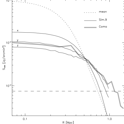
Figure 4: The radial profile (centered on the emission weighted maximum) of the Coma cluster (thick line) is compared to the profiles obtained from the three projections of the simulation shown in Fig. 3 (thin lines). The dotted line represents the mean profile over all ten simulated clusters. The horizontal line marks a crude estimate of the noise enclosed in the observations.

4 Synthetic Radio Maps

To obtain the synthetic radio maps we calculate all quantities needed in a $5\,\mathrm{Mpc}^{3}$ box containing $200^{3}$ grid cells, centered on the cluster position and distribute the CRe as described before. From this data cube we calculate the maps by projecting the emission along the three spatial directions. As the radio emission depends on the angle between the magnetic field and the observing direction, this leads to different total radio luminosities in different observing directions. As the magnetic field in the simulations is nearly isotropic, the differences are small. Additionally projection effects of substructure in the underlying density distribution can lead to different radial profiles as seen in Fig. 4.

As a reference point we chose one simulated cluster (Sim. 9), which has an emission weighted temperature (9.4 keV) and a velocity dispersion (1200 km/s derived from the virial mass and radius) comparable to the values observed in the Coma cluster of galaxies (9 keV (Donelly et al., 1999), 1140 km/s Zabludoff et al. (1993)). This cluster is in a post-merger stadium, like Coma Burns et al. (1994); Bravo-Alfaro et al. (2000).

We assume $\alpha_{p}=2.375$, which gives $\alpha_{\nu}=1.25$, typical for cluster radio halos, and adjust $X_{\rm CRp}$ to $0.14\,{(E_{\rm p,min}/{\rm GeV})}^{-0.375}$ so that this cluster reproduces the observed total 1.4 GHz radio emission of Coma. In the case of a twice the field strength $X_{\rm CRp}$ needs to be $0.04\,{(E_{\rm p,min}/{\rm GeV})}^{-0.375}$. Note that in this case the magnetic fields and the CRp are in equipartition for $E_{\rm p,min}=1\,{\rm GeV}$.

The synthetic radio maps are shown in Fig. 3 in comparison with the radio map of Coma. In the calculation of the radial radio emission profile of Coma the so called radio bridge of Coma (see Fig. 3, top-left panel at $x=3.5$ Mpc, $y=1.5$ Mpc) is included. This can be justified because a similar bridge is also visible in the X-ray emission, which suggests that the radio bridge results from ICM substructure. This substructure is believed to be the core of a smaller merging cluster which already passed the core region of Coma Burns et al. (1994); Bravo-Alfaro et al. (2000). The radio relic in Coma (see Fig. 3, top-left panel at $x=4.5$ Mpc, $y=1$ Mpc) does not affect the comparison of the radio profiles due to its peripheral location.

Although we cannot expect this simulated cluster to match the morphology of the radio halo of Coma exactly, the radial emission profiles in the $y$- and $z$-projection are quite comparable (Fig. 4). In the $x$-projection the two sub-lumps are projected on top of each other. This leads to a steeper radial radio profile (Fig. 4). The second simulated cluster with flat radio emission profile is also in a post-merger stadium with substantial substructure.

The large extension of low level radio emission of Coma is not reproduced by the model. As the simulation has its highest resolution in the center, the simulation might underestimate the small scale magnetic fields, and therefore the radio emission, in the outer regions. This could explain the less extended synthetic radio halo. Another possibility is that e.g. diffusion established a more extended CRp profile than it is assumed in this work.

The observed radio halos do not show any radio polarization. We estimate for our simulated field configuration the expected degree of radio polarization following the treatment of internal Faraday rotation of Burn Burn (1966). The synthetic polarization maps has peak values of the order of $10^{-6}$. This undetectable signal would be further reduced by beam depolarization due to the small-scale polarization pattern.

It is difficult to compare morphological different clusters of galaxies. But Eq. 12 indicates a close relation between radio and X-ray emissivities within the hadronic halo model. This should be approximatively conserved in the projected fluxes, which allows for a less morphology-dependent comparison of different real or simulated clusters. For Sim. 9 we compare X-ray and radio surface brightness point by point. In order to process the data in the same way as real observational data we average over 250 kpc boxes and use the RMS as an error estimate (plus systematic errors of $\delta L_{X}=10^{-7}\,{\rm erg\,s^{-1}\,cm^{-2}}$ and $\delta L_{\nu}=10^{-21}\,{\rm erg\,s^{-1}\,cm^{-2}\,Hz^{-1}}$). The results are given in Fig. 5. For instrumentally detectable regions ($L_{\nu}>\delta L_{\nu}$, $L_{X}>\delta L_{X}$) the radio and X-ray emissivity can be related via a power law $L_{\nu}=a\,L_{X}^{b}$, where $a=2.23\cdot 10^{-13}$ and $b=1.26$ in cgs units. Govoni et al. Govoni et al. (2000) give for four clusters a point by point radio to X-ray count rate correlation. Their values ($b=0.64\pm 0.07$ for Coma, $b=0.82\pm 0.04$ for A2319, $b=0.94\pm 0.04$ for A2255, $b=0.99\pm 0.05$ for A2744) are significantly smaller, which is also supported by the visual impression of the more concentrated simulated halo in comparison to Coma (Fig. 3). This indicates that the radial CRp profile should be more extended than the thermal energy of the ICM, as we have assumed in this work, if radio halos are of hadronic origin.

Figure 5: Point by point radio to X-ray comparison of Sim. 9.

5 Gamma-Rays and Neutrinos

The luminosity of the simulated cluster Sim. 9 in neutrinos and gamma-rays is $Q_{\nu_{{\rm e},\mu}}(E_{\nu})=5.5\cdot 10^{45}\,E_{\nu}^{-2.5}/{\rm GeV^{-1.5}}$ and $Q_{\gamma}(E_{\gamma})=5.9\cdot 10^{45}\,E_{\gamma}^{-2.5}/{\rm GeV^{-1.5}}$. This leads to a gamma ray flux of $\leq 5.2\cdot 10^{-8}{\,\rm cm^{-2}\,s^{-1}}$ above 100 MeV ($\leq$ since the spectrum is significant below the above power law near $E_{\gamma}=100$ MeV). This is comparable to the upper limit $4\cdot 10^{-8}{\,\rm cm^{-2}\,s^{-1}}$ for the flux from Coma measured by EGRET (Sreekumar et al., 1996). In the case of twice the field strength one finds $Q_{\nu_{{\rm e},\mu}}(E_{\nu})=1.5\cdot 10^{45}\,E_{\nu}^{-2.5}/{\rm GeV^{-1.5}}$, and $Q_{\gamma}(E_{\gamma})=1.6\cdot 10^{45}\,E_{\gamma}^{-2.5}/{\rm GeV^{-1.5}}$, which leads to a flux above 100 MeV of $\leq 1.4\cdot 10^{-8}{\,\rm cm^{-2}\,s^{-1}}$ well below the EGRET limit. For comparison with gamma ray and neutrino flux predictions for clusters of galaxies see Völk et al. Volk et al. (1996), Enßlin et al. Enßlin et al. (1997), Colafrancesco & Blasi Colafrancesco & Blasi (1998), and Blasi Blasi (1999).

6 The Temperature-Radio-Luminosity Relation

Clusters with radio halos exhibit a strong correlation between the radio luminosity (at 1.4 GHz: $L_{\rm 1.4GHz}$) and the ICM temperature ($T_{X}$) Liang (1999); Colafrancesco (1999). This is expected because of the known correlations of cluster size and energy content with temperature Mohr & Evrard (1997); Schindler (1999); Mohr et al. (1999). But the shape of the $T_{X}$–$L_{\rm 1.4GHz}$ relation is an important touchstone of every radio halo theory. It can be seen in Fig. 6 that the hadronic halo model reproduces the observed relation if a cluster independent $\varepsilon_{\rm CRp}/\varepsilon_{\rm th}$ ratio is assumed.

Figure 6: Temperature-radio luminosity relation. The data points with the error bars are taken from Liang Liang (1999), the diamonds are the simulated clusters. Bigger symbols mark Coma and Sim. 9.

7 Conclusion

A set of simulated clusters of galaxies in a CDM EdS cosmology, including fully MHD simulated magnetic field structures, was used to test a conceptual simple hadronic secondary electron model for radio halo formation of clusters. The seed magnetic fields were chosen so that the final magnetic fields reproduce the observed Faraday rotation measurements. It was assumed further, that in all clusters a spatially constant ratio between the cosmic ray proton and the thermal energy density exists. We normalized this ratio by comparison of a simulated radio halo of a Coma like cluster in our sample to the observed radio halo of the Coma cluster. With the further simplifying assumption of an unique power law proton energy spectrum, the resulting radio halo, gamma ray and neutrino emission could be calculated. The main results are:

1. A cosmic ray proton to thermal gas energy ratio of 4 … 14 % ${(E_{\rm p,min}/{\rm GeV})}^{-0.375}$ seems to be required to reproduce the total flux at 1.4 GHz of the Coma cluster with the simulated Coma like cluster. $E_{\rm p,min}$ is the lower kinetic energy cutoff of the protons with assumed spectral index $\alpha_{\rm p}\approx 2.375$.

2. The radial profile of the simulated Coma like cluster, is comparable to that of Coma.

3. But a detailed point by point radio to X-ray comparison, reveals a relation ($L_{\rm 1.4GHz}\sim L_{\rm X}^{b}$, $b=1.26$) which seems to be steeper than the observed relation ($b\leq 1$). This would imply that if radio halos are of hadronic origin, the parent cosmic ray proton population needs to have a spatially wider energy density distribution than the thermal gas.

4. The expected radio polarization is of the order of $10^{-6}$. This is mainly a property of the magnetic field configuration, and should also hold for other radio halo models.

5. The expected gamma ray fluxes are below present observational limits, but possibly in the range of future instruments.

6. The set of 10 simulated clusters reproduces the observed radio luminosity-temperature relation of clusters of galaxies surprisingly well.