Comparison of the Two Followup Observation Strategies
for Gravitational Microlensing Planet Searches

Abstract

There are two different strategies of followup observations for the detection of planets by using microlensing. One is detecting the light curve anomalies affected by the planetary caustic from continuous monitoring of all events detected by microlensing survey programs (type I strategy) and the other is detecting anomalies near the peak amplification affected by the central caustic from intensive monitoring of high amplification events (type II strategy). It was shown by Griest & Safizadeh that the type II strategy yields high planet detection efficiency per event. However, it is not known the planet detection rate by this strategy can make up a substantial fraction of the total rate. In this paper, we estimate the relative planet detection rates expected under the two followup observation strategies. From this estimation, we find that the rate under the type II strategy is substantial and will comprise $\sim 1/4$ – 1/2 of the total rate. We also find that compared to the type I strategy the type II strategy is more efficient in detecting planets located outside of the lensing zone. We determine the optimal monitoring frequency of the type II strategy to be $\sim 20$ times/night, which can be easily achieved by the current microlensing followup programs even with a single telescope.

1 Introduction

Experiments to detect microlensing events by monitoring millions of stars located in the Magellanic Clouds and the Galactic bulge have been and are being carried out by several groups (Alcock et al., 1993; Aubourg et al., 1993; Udalski et al., 1993; Alard & Guibert, 1995; Abe et al., 1997). With their efforts, the total number of candidate events now reaches up to a thousand (P. Popowski 1999, private communication).

Although the primary goal for these experiments was to investigate the nature of Galactic dark matter, it turns out to be that microlensing can be very useful in various other fields of astronomy. One of the important applications of microlensing is the detection of extra-solar planets. Planet detection by using microlensing is possible because the event caused by a lens system with a planet can exhibit detectable anomalies in the light curve when the source passes close to the lens caustics (Mao & Paczyński, 1991; Gould & Loeb, 1992; Bolatto & Falco, 1994). For this lens system, there are 2 or 3 disconnected sets of caustics depending on the projected separation between the planet and the primary lens (planet-lens separation). Among them, one is located very close to the primary lens, ‘central caustic’, and the other(s) is (are) located relatively away from the primary lens, ‘planetary caustics’ (Griest & Safizadeh, 1998). Accordingly, there exist two different types of anomalies in the light curves; one affected by the planetary caustic(s), ‘type I anomaly’, and the other affected by the central caustic, ‘type II anomaly’ (Covone et al., 2000). Due to the characteristics of the central caustic, type II anomalies occur near the peak of the light curves of high amplification events.

Compared to the frequency of type I anomalies, type II anomalies occur with a relatively low frequency due to the smaller size of the central caustic than the corresponding planetary caustic. However, the efficiency of detecting type II anomalies can be high because intensive monitoring of events is possible due to the predictable time of anomalies (Griest & Safizadeh, 1998). We call the planet search strategy of intensive monitoring near the peak of high amplification events as the ‘type II’ strategy, while the strategy of continuous monitoring for all events detected from lensing survey programs as the ‘type I’ strategy. Then a naturally arising questions is whether the planet detection rate (not the detection efficiency per event) under the type II strategy can make up a substantial fraction of the total rate. In this paper, we answer to this question by estimating the relative detection rates under the two strategies of planet search followup observations.

2 Types of Planet-induced Anomalies

The lens system with a planet is described by the formalism of the binary lens system with a very low-mass companion. When lengths are normalized to the combined angular Einstein ring radius, which is equivalent to the angular Einstein ring radius of a single lens with a mass equal to the total mass of the binary, the lens equation in complex notations for a binary lens system is represented by

$$\zeta=z+{m_{1}\over\bar{z}_{1}-\bar{z}}+{m_{2}\over\bar{z}_{2}-\bar{z}},$$ (1)

where $m_{1}$ and $m_{2}$ are the mass fractions of individual lenses (and thus $m_{1}+m_{2}=1$), $z_{1}$ and $z_{2}$ are the positions of the lenses, $\zeta=\xi+i\eta$ and $z=x+iy$ are the positions of the source and images, and $\bar{z}$ denotes the complex conjugate of $z$ (Witt, 1990). The combined angular Einstein ring radius is related to the physical parameters of the lens system by

$$\theta_{\rm E}=\left({4GM\over c^{2}}{D_{\rm ls}\over D_{\rm os}D_{\rm ol}}\right)^{1/2},$$ (2)

where $M$ is the total mass of the binary lens system and $D_{\rm ol}$, $D_{\rm ls}$, and $D_{\rm os}$ represent the separations between the observer, lens, and source star, respectively. The amplification of each image is given by the Jacobian of the transformation (1) evaluated at the image position, i.e.

$$A_{i}=\left({1\over|{\rm det}\ J|}\right)_{z=z_{i}};\qquad{\rm det}\ J=1-{\partial\zeta\over\partial\bar{z}}{\overline{\partial\zeta}\over\partial\bar{z}}.$$ (3)

Then the total amplification of a binary lens event is given by the sum of the amplifications of the individual images, i.e. $A=\sum_{i}A_{i}$. The set of source positions with infinite amplifications, i.e. ${\rm det}\ J=0$, form closed curves called caustics. As a result, whenever a source passes very close to the caustic, the resulting light curve deviates significantly from the standard Paczyński (1986) curve.

The caustic structure of the lens system with a planet varies depending on the planet-lens separation $d$ normalized by $\theta_{\rm E}$. A lens system with a wide planet ($d>1.0$) forms 2 disconnected sets of caustics. One caustic is located very close to the center of mass (and thus referred as the central caustic), and the other planetary caustic is located away from the center of mass on the planet-side (with respect to the center of mass) axis connecting the primary lens and the planet. A system with a close planet ($d<1.0$) also has a single central caustic, but has two planetary caustics, which are located on the opposite side of the planet with respect to the center of mass and not on the planet-lens axis. The sizes of both the central and planetary caustics are maximized when the planet is located in the lensing zone of $0.618\leq d\leq 1.618$ (Griest & Safizadeh, 1998), and decrease as the planet-lens separation becomes either smaller or larger. However, regardless of the separation the central caustic of a lens system is always smaller than the corresponding planetary caustic(s).

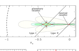
Figure 1: The central and planetary caustics of an example lens system with a planet and the corresponding type I and II anomalies in the resulting light curves. Presented in upper panel is the contour map of the fractional amplification excess $\epsilon$. The contours around the individual types of caustic (closed figures drawn by the thick solid line) are drawn at the levels of $\epsilon=1\%$, 5%, and 10%. The example lens system has a mass ratio and a planet-lens separation of $q=10^{-3}$. The lower panels show the light curves resulting from the two source trajectories marked by straight lines in the upper panel. The two curves in each panel represent those expected in the presence (solid curve) and absence (dotted curve) of the planet, respectively.

In Figure 1, we illustrate the central and planetary caustics of an example lens system with a planet and the corresponding type I and II anomalies in the resulting light curves. Presented in upper panel are the contour map of the fractional amplification excess, which is computed by

$$\epsilon={\left|A-A_{\rm s}\right|\over A_{\rm s}},$$ (4)

where $A$ and $A_{\rm s}$ represent the amplifications with and without the existence of the planet, respectively. The single lens event amplification is related to the separation (normalized by the angular Einstein ring radius of the primary lens) between the source and the primary lens, $u$, by

$$A_{\rm s}={u^{2}+2\over u(u^{2}+4)^{1/2}}.$$ (5)

The contours (thin solid curves) around the individual types of caustic (closed figures drawn by the thick solid line) are drawn at the levels of $\epsilon=1\%$, 5%, and 10% with increasing distance from the caustics. The example lens system has a mass ratio and a projected planet-lens separation of $q=10^{-3}$ (corresponding to a Jupiter-mass planet around a $1\ M_{\odot}$ star) and $d=1.2$. The positions of the primary lens and the planet are chosen such that the center of mass is at the origin and all lengths are scaled by $\theta_{\rm E}$. The lower panels show the light curves resulting from the two source trajectories marked by straight lines in the upper panel. The two curves in each panel represent those expected in the presence (solid curve) and absence (dotted curve) of the planet. Times are in units of the Einstein ring radius crossing time (Einstein time-scale). From the figure, one finds that the region of large type II deviations is smaller than the corresponding region of type I deviations. One also finds that the type II anomaly in the light curve occurs near the peak amplification.

3 Type I versus Type II Strategies

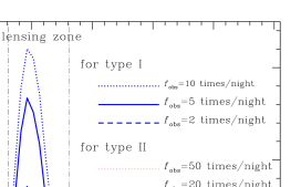
Figure 2: Distributions of the planet detection probability expected under the type I and II followup observation strategies with various monitoring frequencies as a function of the planet-lens separation for events caused by a planetary system with $q=10^{-3}$. The events are assumed to have $t_{\rm E}=20\ {\rm days}$. The region enclosed by the dot-dashed lines represents the lensing zone with $0.618\leq d\leq 1.618$. For the details about the observational conditions and detection criteria, see the text.

Table 1: The Fractions of Planet Detections by the Type II Strategy

$f_{\rm obs}$		fraction (%)
(times/night)		for all systems	for systems with
type I	type II	with $d\leq 5.0$	$d$ in the lensing zone
2	10	45.2	37.6
	20	52.1	40.5
	50	53.6	41.3
5	10	34.8	27.9
	20	41.3	30.4
	50	42.8	31.1
10	10	30.9	23.9
	20	36.4	26.3
	50	37.8	26.8

Note. — The fractions of planet detection rate under the type II strategy out of the total rate for various combinations of monitoring frequencies of the individual strategies. Two sets of fractions are presented. The first set is for all planetary systems with planet separations $d\leq 5.0$ and the second set is for those with planets located in the lensing zone only.

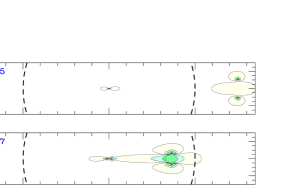
Figure 3: The variation in the positions of the type I and II deviation regions. Notations are same as those in the upper panel of Figure 1.

Due to the difference in the characteristics of the central and planetary caustics and the resulting anomalies, detecting planets by using the type II strategy has both advantages and disadvantages. The greatest advantage of the type II strategy is that the time of anomalies, which occurs near the peak amplification, can be predicted in advance, and thus high time-resolution monitoring of the event is possible (Griest & Safizadeh, 1998). In addition, more accurate photometry can be performed because more photons will be available for high amplification events. On the other hand, the disadvantage is that type II anomalies occur with a relatively low frequency due to the smaller size of the central caustic. Then, the question is whether the planet detection rate under the type II strategy can be high enough to be comparable to the rate under the type I strategy. In this section, we answer to this question by estimating the relative planet detection rates expected under the two different types of planet search strategies.

To estimate the detection rates, we assume the following observational conditions and detection criteria. For the type I strategy, all events with $A\mathrel{\hbox{\hbox to0.0pt{\hbox{\lower 4.0pt\hbox{$\sim$}}\hss}\hbox{$>$}}}A_{\rm th}=1.34$ (i.e. $u\leq u_{\rm th}=1.0$) are assumed to be monitored in a round-the-clock manner during 8 hours per night on average. Here $u_{\rm th}$ and $A_{\rm th}$ represent the threshold lens-source separation and the corresponding threshold amplification, which are required for the event to become the target of followup observations. On the other hand, if the events are suspected to have high amplifications with $A\geq A_{\rm th}=10$ (i.e. $u\mathrel{\hbox{\hbox to0.0pt{\hbox{\lower 4.0pt\hbox{$\sim$}}\hss}\hbox{$<$}}}u_{\rm th}=0.1$), they become targets for intensive montoring by the type II strategy. We assume that the type I strategy is employed during $-0.4t_{\rm E}\leq t_{\rm obs}\leq 2.0t_{\rm E}$, while the type II strategy is employed only during the time of high amplifications with $A\geq A_{\rm th}$. For planet detection, it is assumed that one should detect light curve deviations greater than a threshold value, $\epsilon_{\rm th}$, at least more than 5 times. The adopted threshold deviations are $\epsilon_{\rm th}=5\%$ for the type I and $1\%$ for the type II strategies, respectively. We adopt the lower value of $\epsilon_{\rm th}$ for the type II strategy because the events monitored by this strategy will have higher amplifications. For more sophisticated computations of the planet detection probability including not only more refined models of photometric precision but also the effects of finite source size and blending, see Gaudi & Sackett (2000). According to the current microlensing detection rate, there are on average several dozens of on-going events. Then, considering the average total observation time of $\sim 8$ hours per night and $\sim 5$ – 10 minutes of required time per event, one can observe on average $\sim 2$ – 3 times for each event under the type I strategy. However, since the frequency can be increased by employing multiple telescopes like the current followup observation teams (Albrow et al., 1998; Rhie et al., 1999), we test various monitoring frequencies per night of $f_{\rm obs}=2$, 5, and 10 for the type I strategy. For the type II strategy, we test $f_{\rm obs}=10$, 20, and 50.

In Figure 2, we present the distributions of the planet detection probability expected under the individual strategies with various monitoring frequencies as a function of the planet-lens separation for events caused by a planetary lens system with $q=10^{-3}$. The events are assumed to have a common Einstein time scale of $t_{\rm E}=20\ {\rm days}$, which corresponds to that of the bulge self-lensing event with a lens mass $1\ M_{\odot}$. The region enclosed by the dot-dashed lines represents the lensing zone. Note that our probability under the type II strategy are normalized by the total number of events with $A\geq 1.34$ unlike those of Griest & Safizadeh (1998), who normalized by the number of only the intensively monitored high amplification events. Since we applied $u_{\rm th}=0.1$, our probability is equivalent to approximately one tenth of their value. In Table 1, we list the fractions of planet detection rate by the type II strategy out of the total rate (type I + type II) for various combinations of $f_{\rm obs}$ of the individual strategies. We estimate two sets of fractions. The first set is for all planetary systems with separations $d\leq 5.0$ and the second set is for those with planets located within the lensing zone only.

The findings from Figure 2 and Table 1 are summarized as follows:

1. As pointed out by Griest & Safizadeh (1998), the planet detection efficiency per event, which is ten times of the probability presented in Figure 2, expected under the type II strategy is very high. We note, however, that our estimate is somewhat lower than their estimate. We suspect the difference is caused because they assume that the type II monitoring strategy is applied during the entire duration of the event, while we assume that intensive monitoring is performed only during the time of high amplifications. We actually obtain similar efficiency distributions to theirs under the observational conditions they assumed.

2. In addition to the higher efficiency, the planet detection rate under the type II strategy is expected to comprise a substantial fraction of the total rate. We find that the fraction will be $\sim 1/4$ – 1/2 depending on the combinations of the individual strategies’ monitoring frequencies.

3. Compared to the type I strategy, the type II strategy is more efficient in detecting planets located outside of the lensing zone. This is because while the planetary caustic lies at the position with increasing distance from the primary lens as the planet-lens separation becomes smaller or large than $d\sim 1.0$ (Wambsganss, 1997), the central caustic is located always near the primary lens regardless of the planet-lens separation (see Figure 3). As a result, while the type II efficiency decreases only by the decrease of the (central) caustic size, the type I efficiency is decreased additionally by the increasing distance of the (planetary) caustic location from the primary lens.

4. The optimal monitoring frequency of the type II strategy will be $f_{\rm obs}\sim 20$. This is because observations with frequencies higher than this value will result in very slight increase in the planet detection rate (see Table 1). This optimal frequency can be easily achieved by the current followup programs even with a single telescope.

4 Conclusion

We compare the planet detection rates expected by the type I and II followup observation strategies. From this comparison, we find that the rate under the type II strategy will be substantial, comprising $\sim 1/4$ – 1/2 of the total rate. It is also found that compared to the type I strategy, the type II strategy is more efficient in detecting planets located outside of the lensing zone. Therefore, in addition to yielding high planet detection efficiency for each high amplification event, employment of the type II strategy will allow one not only to increase the total planet detection rate but also to probe the existence of planets with a wider range of separations. Despite these benefits, implementation of the strategy requires only a modest improvement in the monitoring frequencies.

References

- Abe et al. (1997) Abe, F., et al. 1997, in Variable Stars and the Astrophysical Returns of the Microlensing Surveys, eds. R. Ferlet, J.-P. Milliard, & B. Raba (Cedex: Editions Frontieres), 75
- Alard & Guibert (1995) Alard, C., & Guibert, J. 1997, A&A, 326, 1
- Albrow et al. (1998) Albrow, M. D., et al. 1998, ApJ, 509, 687
- Alcock et al. (1993) Alcock, C., et al. 1993, Nature, 365, 621
- Aubourg et al. (1993) Aubourg, E., et al. 1993, Nature, 365, 623
- Bolatto & Falco (1994) Bolatto, A. D., & Falco, E. E. 1994, ApJ, 436, 112
- Covone et al. (2000) Covone, G., de Ritis, R., Dominik, M., & Marino, A. A. 2000, A&A, 357, 816
- Gaudi & Sackett (2000) Gaudi, B. S., & Sackett, P. D. 2000, ApJ, 528, 56
- Gould & Loeb (1992) Gould, A., & Loeb, A. 1992, ApJ, 396, 104
- Griest & Safizadeh (1998) Griest, K., & Safizadeh, N. 1998, ApJ, 500, 37
- Mao & Paczyński (1991) Mao, S., & Paczyński, B. 1991, ApJ, 374, L37
- Paczyński (1986) Paczyński, B. 1986, ApJ
- Rhie et al. (1999) Rhie, S. H. 1999, ApJ, 522, 1037
- Udalski et al. (1993) Udalski, A., et al. 1993, Acta Astron., 43, 289
- Wambsganss (1997) Wambsganss, J. 1997, MNRAS, 284, 172
- Witt (1990) Witt, H. J. 1990, A&A, 263, 311