Comparing Giant Molecular Clouds in M31, M33 & the Milky Way

Abstract

We present new observations of a 2^′ field in the north-eastern spiral arm of M31. In the 0.8 $\times$ 3.6 kpc mosaicked region, we have detected six distinct, large complexes of molecular gas, most of which lie along the spiral arm dust lane or in the vicinity of HII regions. The mean properties of these complexes are as follows: D$\sim$57$\pm$13 pc, $\Delta$V$\sim$ 6.5$\pm$1.2 km s^-1, M_CO$\sim$3.0$\pm$1.6 $\times$10⁵ $M_{\hbox{$\odot$}}$, peak brightness temperatures$\sim$1.6–4.2 K. We investigate the effects of spatial filtering on the quantitative comparison of Local Group and Milky Way giant molecular clouds properties and distributions. We also discuss different cloud identification techniques and their impact on derived cloud properties. When we employ the same cloud identification method and account for differences in data acquisition for M31, Milky Way, and M33, we find that the molecular cloud complexes in all three galaxies are similar. While the global distribution of molecular gas may vary from galaxy to galaxy, cloud complexes are similar, suggesting that cloud formation and destruction is determined by local physics. This work is supported by grants AST-9613716 & AST-9981289 from the National Science Foundation.

1 Introduction

Molecular gas is a major constituent of the interstellar medium in the inner disks of spiral galaxies. It is organized into discrete entities (clouds and cloud complexes) and virtually all star formation is associated with them (see reviews by Scoville 1990; Combes 1991; Blitz 1993). However, the molecular cloud populations and properties in external galaxies are not well known because of the difficulty in obtaining the high resolution, high sensitivity data required for spatially resolving individual complexes. For instance, in the nearest spiral M31, a typical molecular cloud ($\sim$40 pc) has an angular size of 12^′′, comparable to the beam of the world’s largest single dish millimeter-wavelength telescope in the CO(1-0) line.

Interferometric observations can achieve the higher resolution necessary, and with improved receiver technology and other advances, several molecular clouds have been detected in both M31 (Vogel, Boulanger & Ball 1987; Wilson & Rudolph 1993) and M33 (Wilson & Scoville 1990, 1992). With forthcoming arrays like CARMA and ALMA, it will be possible to study molecular clouds over the entire disks of galaxies as far away as the Virgo cluster. In order to compare such interferometric observations with Milky Way studies, we must understand the effects of spatial filtering of interferometers. In addition, we must understand which if any of the various methods of identifying molecular clouds are appropriate for comparing clouds in different galaxies. In this contribution, we address these issues by comparing molecular clouds using new and existing data for M31, M33 and the Milky Way.

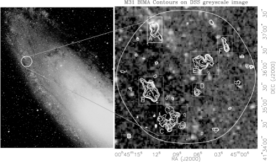
Fig. 1: Velocity-integrated intensity map of M31 field shown in logarithmic contours of 1.5${}^{n}\times$ 2 K km/s. The grey scale image underlying the contours is a DSS image in which obscuring dust appears black. The six complexes used for comparison to the Milky Way are identified with the boxes labelled A-F. The outer circle is the gain=0.4 contour.

2 Data: New M31 Observations & Existing Data

In Figure 1, we show a velocity-integrated CO(J=1–0) BIMA (Berkeley-Illinois-Maryland Association) map in contours overlaid on a grey-scale optical image. Most of the CO emission lies in the two dust lanes which are separated by a distance of 2 kpc (assuming $i$=77^o). Our mass sensitivity limit for these data is 5$\times$10⁴$M_{\hbox{$\odot$}}$. We also obtained the interferometric OVRO data for M33 (Wilson & Scoville 1990) and parts of the 1.2m Columbia Survey (Dame et al. 1987) for four large ($\sim$10⁵-10⁶$M_{\hbox{$\odot$}}$) Milky Way complexes: Gem OB1 (Stacy & Thaddeus 1991), W3 (Digel et al. 1996), Cas A (Dame et al. 1987), and a complex in the outer Carina arm (Grabelsky et al. 1987).

3 Comparing GMCs in M31, M33 and the Milky Way

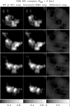
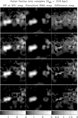
Fig. 2: Simulation of interferometric observations of the Gem OB1 complex (left) and the outer Carina Arm complex (right). In each panel, the 4 rows represent consecutive channels from the data cube, The first column shows the Milky Way data projected at M31, the middle column shows the same data (with same greyscale) after simulated observations with BIMA, and the third column shows the difference between the first and second columns.

3.1 Spatial Filtering Experiments: Milky Way Clouds Moved to M31

For both interferometers and single dish telescopes, the observed brightness distribution is the convolution of true brightness with the instrument response function. This response is qualitatively different for the two types of telescopes. In general, interferometers are better at mapping small, compact structures than smooth, large angular-size structures. To evaluate the effect of the observational method on determination of cloud properties, we simulated interferometric observations of the Milky Way complexes at the distance of M31. Our simulations found that Gem OB1, W3 and Cas A complexes were recovered completely by the interferometer; their sizes, shapes and velocity widths were identical before and after the interferometric observations (see left panel in Fig. 2). In contrast, the complex in the outer Carina Arm suffered from a significant loss of flux (as much as $\sim$50%) but the complex itself did not change shape, size or velocity width (see right panel in Fig. 2).

The difference between the three complexes recovered completely and the Carina complex is that the Carina complex is $\sim$ 4$\times$ further away. At this distance, the 8$.\mkern-4.0mu^{\prime}$8 beam of the 1.2m telescope is not able to provide a sufficiently high resolution map to mimic the true distribution of the molecular gas; the complex is smoothed by the coarse beam and consequently the flux is resolved out by the interferometer. To test whether this was indeed the case, we smoothed the Cas A complex and projected it to the distance of M31 and observed it with the interferometer; the result was the same as for the Carina complex: as much as 50% of the flux was resolved out. Thus we conclude that interferometers are excellent instruments for recovering typical Milky Way GMCs and interferometric M31 and M33 data may be compared to the single dish MW data.

3.2 Cloud Identification Experiments: What is a Molecular Cloud?

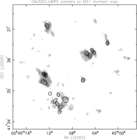
Fig. 3: Illustration of differences between Method I and II. The edges of the grey scale would be the individual complexes defined by Method I as shown in Figure 1 where the complexes A-F are defined using this method. The black ovals are clouds identified by Gaussclumps, i.e. Method II.

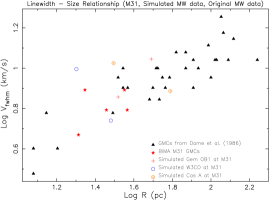
Fig. 4: Comparison of M31 and Milky Way clouds using Method I. The size-linewidth relationship is the same for MW clouds (triangles, Dame et al. 1986), M31 (stars, BIMA observations), and the simulated Milky Way complexes (other symbols).

The techniques for identifying clouds can be divided broadly into two main methods with opposite philosophies. The first method defines clouds using an integrated intensity contour, ignoring all substructure (e.g., Dame et al. 1986; Sanders et al. 1985). The second method identifies as clouds all resolved intensity peaks which emphasizes the substructure in molecular emission (e.g, Gaussclump by Stutzki & Güsten 1990 or Clumpfind by Williams et al. 1994). The difference between these methods is illustrated in Figure 3. The advantage of the first method is that the results can be directly compared to several previous Galactic studies of GMCs. However this method is time consuming and subjective. In contrast, the second method can be automated, but it has a severe drawback in that it never identifies clouds larger than one or two resolution elements. This resolution dependence, while useful for studying the substructure in the molecular ISM, makes comparative studies of GMCs in different galaxies difficult. We applied both methods to the simulated Milky Way data, and the M31 and M33 datasets.

Method I. Using an integrated intensity contour: We defined M31 complexes using the integrated intensity contour method. These are the complexes A-F in Fig.1. Comparing these to those found in the Milky Way by Dame et al. (1987) using a similar technique, we find that the M31 complexes are very similar to the Milky Way complexes. In our data, M31 complexes range in sizes from 40–75 pc and have velocity widths 4.7–7.8 km s^-1(FWHM), compared to the Milky Way complexes which ranged from 20–250 pc and 4-15 km s^-1. The M31 clouds appear to be virialized, i.e. their virial masses are equal to their molecular masses within a factor of 2 (calculated with N(H₂)/W_CO= 3$\times$10²⁰ cm^-2 K^-1 km^-1 s). The M31 complexes have masses ranging from 0.8–5$\times$10⁵$M_{\hbox{$\odot$}}$. We find that the M31 complexes follow the same linewidth-size relationship as the Milky Way complexes (see Figure 4). Applying this method to the M33 data, we find that the Wilson & Scoville (1990) clouds increase in size because neighbouring clumps are now identified as a single complex; complexes thus defined have properties similar to those seen in M31 and Milky Way complexes.

Method II. Using Gaussclump: Since the simulated Milky Way data has similar resolution and noise characteristics as the M31 and M33 datasets, we compared all three using Gaussclump. We found that the derived properties (amplitude, velocity widths and sizes) of all three datasets were similar (figure not shown). But as noted earlier, these methods measure the substructure in molecular clouds rather than their overall properties, and therefore cannot be used to characterize global populations and properties of GMCs in a galaxy. Nonetheless, applying both methods leads to the same conclusion: the GMCs in all three galaxies are fairly similar.

SUMMARY: By simulating interferometric observations of Milky Way GMCs at Andromeda, we concluded that interferometers are excellent at recovering GMCs in M31 and M33. Then by using common cloud identification techniques, we found that GMCs in all three galaxies are similar to each other. Surveys much larger than ours will be necessary for determining global properties (e.g., mass distribution functions) of GMC populations.

References

Blitz, L. (1993) in Protostars and Planets III, ed. Levy, E.H. & Lunine, J.I. p. 125-161

Combes, F. (1991) Annu. Rev. Astron. Astrophys. 29, 195

Dame, T.M., Elmegreen, B.G., Cohen, R.S., & Thaddeus, P. (1986) , Astrophys. J., 305892.

Dame, T.M., Ungerechts, H., Cohen, R.S., de Geus, E.J., Grenier, I.A., May, J., Murphy, D.C., Nyman, L.-A., Thaddeus, P. (1987) Astrophys. J. 322, 706.

Digel, S.W., Lyder, D.A., Philbrick, A.J., Puche, D., & Thaddeus, P. (1996) Astrophys. J. 458, 561.

Grabelsky, D.A., Cohen, R.S., Bronfman, L., Thaddeus, P., & May, J. (1987) Astrophys. J. 315, 122.

Sanders, D.B., Scoville, N.Z., Solomon,P.M. (1985) Astrophys. J. 289, 373.

Scoville, N.Z. (1990) in The Evolution of the Interstellar Medium, ed. L. Blitz, PASP, p. 49.

Stacy, J.A., Thaddeus, P. (1991) in ASP Conf. Ser. 16, Atoms, Ions, and Molecules: New Results in Spectral Line Astrophysics, eds. A. D. Haschick & P.T.P. Ho, ASP, p. 197

Stutzki, J., & Güsten, R. (1990) Astrophys. J. 356, 513.

Vogel, S.N., Boulanger, F., & Ball, R. (1987) Astrophys. J. 321, 145

Williams, J.P., de Geus, E.J., & Blitz, L. (1994) Astrophys. J. 428, 693.

Wilson, C.D., & Rudolph, A.L. (1993) Astrophys. J. 406, 477

Wilson, C.D., & Scoville, N. (1990) Astrophys. J. 363, 435.

Wilson, C.D., & Scoville, N. (1990) Astrophys. J. 385, 512.