A new look at simple inhomogeneous chemical evolution

Abstract

A rudimentary, one-zone, closed-box model for inhomogeneous chemical evolution is offered as an alternative reference than the Simple model in the limit of no mixing. The metallicity distribution functions (MDFs) of Galactic halo and bulge stars can be matched by varying a single evolutionary parameter, $nQ$. $Q$ is the filling factor of contaminating regions and $n$ is the number of star-forming generations. Therefore, Q and n have equivalent roles, and combinations of $n$ and $Q$ yield systems with different metallicities at any given age. The model also revises interpretation of observed MDFs. Unevolved systems probe the parent distribution of metal production $f(z)$, for example, the high-metallicity tail of the halo distribution agrees with a power-law $f(z)$.

1. Introduction

The relation between galactic star formation history and the interstellar medium (ISM) is recorded in the distribution of elements we observe today. The principal signatures are: (A) Time-integrated metallicity distribution functions (MDFs), as exhibited by long-lived stars; (B) instantaneous MDFs at a given time, for example, the present-day dispersion in the inhomogeneous ISM; (C) abundance ratios of elements with varying origin and histories; and (D) age-metallicity relations. A unified understanding of these tracers is fundamental to solving the puzzle of galaxy assembly and evolution.

Over the 30 years of work on chemical evolution modeling, the constraints offered by (B), the instantaneous MDF, have been relatively neglected. However, Tinsley (1975) showed early on that chemical inhomogeneity significantly affects the other chemical signatures. Edmunds (1975) also argued that simplistic inhomogeneous evolution of overlapping supernova remnants, with no mixing, yields a present-day ISM that is orders of magnitude smoother than what is presently observed. This issue is only rarely discussed (e.g., Roy & Kunth 1995). But recently, the significance of dispersions in the chemical signatures has been reemphasized (e.g., Wyse 1995; van den Hoek & de Jong 1997). We are therefore overdue to reexamine inhomogeneous chemical evolution.

Picking up threads from the early work, I present here an analytic model that predicts the metallicity dispersion from first principles in the limiting case of no mixing. As a reference, we return to the standard, Simple model (e.g., Tinsley 1980; Pagel & Patchett 1975; Schmidt 1963), which assumes: (1) a closed system, (2) initially metal-free, (3) constant stellar initial mass function (IMF), and (4) chemical homogeneity at all times. Most previous analytic investigations of inhomogeneous evolution were tied to the Simple model, and assumed a given dispersion in metal production: Tinsley (1975) adopted a fixed metallicity dispersion and propagated this through the Simple model; while Searle (1977) and Malinie et al. (1993) considered an ensemble of regions that individually follow the Simple model such that they yield a given dispersion.

2. A fresh approach

A different, perhaps simpler, approach, returns to the concept of overlapping regions of contamination, as discussed qualitatively by, e.g, Edmunds (1975). We adopt the tenets, except for (4), of the Simple model. Consider an initially metal-free ISM, in which a first generation of star forming regions is randomly distributed, occupying a volume filling factor $Q$. We assume that these individual regions have a distribution of metal production $f(z)$, which is the probability density function for obtaining metallicity $z$ at any point affected by star formation. Note that it is not necessary to assume anything specific about the sizes of the individual regions, but only the relative total volumes of contaminated to primordial gas, given by $Q$.

We now consider $n$ subsequent generations of star formation. The individual regions also fall randomly in the ISM, but for each generation, occupy the same filling factor $Q$ as the first. The role of this last assumption will become apparent in §4 below. The probability that any given point in the ISM is occupied by $j$ overlapping regions is given by the binomial distribution in $n$ and $Q$:

$$P_{j}=\Biggl{(}{n\atop j}\Biggr{)}\ Q^{j}\ (1-Q)^{n-j}\ \ ,\quad 1\leq j\leq n\quad;$$ (1)

and the probability of a point retaining primordial metallicity is,

$$P_{0}=(1-Q)^{n}\quad.$$ (2)

For our purposes, we define the metallicity $z$ to be the mass of metals per unit volume; the coexisting mass density of H is assumed to be spatially uniform. In accordance with our assumption of no mixing, we assume that the metallicity at any given point is the sum of those contributed by the individual overlapping regions $z_{i}$:

$$z=\sum_{i=1}^{j}\ z_{i}\quad.$$ (3)

To obtain the instantaneous MDF after $n$ generations, we sum the distributions $N_{j}(z)$ for individual sets of regions occupied by $j$ objects, weighted by their $P_{j}$:

$$N_{\rm ins}(z)=\sum_{j=1}^{n}\ P_{j}\ N_{j}(z)\quad.$$ (4)

To derive the total MDF of all objects ever created over $n$ generations, we must reduce the total gas mass after each generation $k$ by a factor $D_{k}=1-k\delta$, to account for the conversion of gas into stars. We assume the reduction increment $\delta$ to be constant, so that the present-day gas fraction $\mu_{1}=1-n\delta$. The total, time-integrated MDF is then:

$$N_{\rm tot}(z)=\frac{1}{n}\ \sum_{k=1}^{n}\ D_{k-1}\ N_{\rm ins,k}(z)=\frac{1}{n}\ \sum_{j=1}^{n}\ \sum_{k=j}^{n}\ D_{k-1}\ P_{j,k}\ N_{j}(z)\ ,$$ (5)

where $P_{j,k}$ is $P_{j}$ for a given generation $k$. Note that this treatment for gas consumption assumes that $P_{j,k}$ remain unaffected by the reduction of gas.

We now assume that $f(z)$ remains the same for all generations. For large $j$, the Central Limit Theorem applies, which predicts that the summed MDF approximates a normal distribution with mean and variance given by $j$ times the mean $a$ and variance $\sigma^{2}$ of $f(z)$. Thus, $N_{\rm ins}(z)$ is given simply by:

$$N_{\rm ins}(z)=\sum_{j=1}^{n}\ P_{j}\ (2\pi j\sigma^{2})^{-1/2}\ e^{\frac{-(z-ja)^{2}}{2j\sigma^{2}}}\quad,$$ (6)

where $P_{j}$ is given by equation 1. Likewise, to estimate $N_{\rm tot}(z)$ for large $k$, the binomial distribution approximates a normal distribution with mean and variance given by

$$a_{\rm b} = kQ$$

$$\sigma_{\rm b}^{2} = kQ(1-Q)\quad.$$ (7)

Thus equation 5 may be written:

$$N_{\rm tot}(z)=\frac{1}{n}\ \sum_{j=1}^{n}\ \sum_{k=j}^{n}\frac{D_{k-1}}{j^{1/2}\ 2\pi\sigma_{\rm b}\sigma}\ e^{\frac{-(j-a_{\rm b})^{2}}{2\sigma_{\rm b}^{2}}\ +\frac{-(z-ja)^{2}}{2j\sigma^{2}}}\ \ .$$ (8)

For small $n$, equations 6 and 8 break down unless $f(z)$ describes a normal distribution.

3. The form of $f(z)$

Several considerations suggest that $f(z)$ should be given by a power-law. As a rough estimate, we consider the volume affected by a star-forming region to be that of the superbubble generated by its $N_{*}$ core-collapse supernovae (SNe). Following Oey & Clarke (1997; hereafter OC97), the mechanical power $L=N_{*}E_{\rm SN}/t_{\rm e}$, where $t_{\rm e}=40$ Myr is the life expectancy of $L$ for OB associations, and $E_{\rm SN}=10^{51}$ erg is the individual SN energy. The mechanical luminosity function of $L$ is assumed to be a power-law with index $-\beta$ (OC97, eq. 1). If the superbubbles grow until they are confined by the ambient pressure, the standard, adiabatic shell evolution implies that their final radii will be related to $L$ as $R\propto L^{1/2}$ (OC97, eq. 29). The total affected volume is therefore,

$$V_{s}\propto R^{3}\propto L^{3/2}\quad.$$ (9)

In contrast, the total mass of metals produced by $N_{*}$ SNe is given by,

$$M_{z}=m_{y}\ (t_{\rm e}/E_{\rm SN})\ L\quad,$$ (10)

where $m_{y}$ is the mean yield of metals per SN.

Taking $z=M_{z}/V_{s}$, we find that $z\propto L^{-1/2}$ for the superbubble population, showing that the largest superbubbles generate the lowest metallicities, owing to dilution into larger volume. The MDF for superbubbles is,

$$N_{s}(z)\ dz\propto N_{s}(R)\ dR\ \frac{dz}{dR}\propto z^{-3+2\beta}dz\propto z\ dz\quad,$$ (11)

where $N_{s}(R)\propto R^{1-2\beta}$ is the size distribution for objects at their final radii (OC97, eq. 41). The final relation is obtained for $\beta=2$, a value typical, perhaps, for all galaxies (Oey & Clarke 1998). Here we see that there are larger numbers of metal-rich objects owing to the larger numbers of smaller superbubbles. Finally, the probability density for $z$ at any given point in the ISM is:

$$f(z)\propto\frac{4}{3}\pi R^{3}\ N_{s}(z)\propto z^{-6+2\beta}\quad.$$ (12)

For $\beta=2$, we obtain,

$$f(z)\ dz=Cz^{-2}\ dz\ \ ,\quad z_{\rm min}<z<z_{\rm max}\quad.$$ (13)

Since $f(z)$ is a probability density function, its integral must be unity, and $C$ gives the appropriate normalization. Thus, for a given generation of star formation, $f(z)$ is weighted toward low-metallicity regions because of their large sizes. The limiting values $z_{\rm min}$ and $z_{\rm max}$ are determined by the corresponding $R_{\rm max}$ and $R_{\rm min}$.

For a Salpeter (1955) IMF of slope –2.35 and SN progenitor masses between 8 and 120 $\rm\,M_{\odot}$, we use $m_{y}=10\ \rm\,M_{\odot}$, based roughly on models by Woosley & Weaver (1995). We take $R_{\rm max}=1300$ pc, a rather arbitrary value corresponding to the characteristic parameter $R_{\rm e}$ of OC97; and $R_{\rm min}=25$ pc, corresponding to individual SN remnants. These yield $\log z_{\rm min}=-4.7$ and $\log z_{\rm max}=-3.0$, or, taking O as a tracer of primary elements, minimum and maximum [O/H] of –3.0 and –1.3 relative to solar. The adopted yield of $m_{y}=10\rm\,M_{\odot}$ may be somewhat high (e.g., Woosley & Weaver 1995), but the mean $f(z)$ may be somewhat modified depending on $z_{\rm min}$ and $z_{\rm max}$.

4. Results

We can now construct Monte Carlo models of the MDF for small $n$. We generate the components $N_{j}(z)$ by drawing from $f(z)$ (equation 13) $j$ times and summing the drawn $z_{i}$ (equation 3). This is repeated 5000 times to obtain distributions for $N_{j}(z)$. Equations 4 and 5 then provide the instantaneous and total MDFs. The histograms in Figures 1$a$ and $c$ show these models of $N_{\rm ins}(z)$ and $N_{\rm tot}(z)$ for $n=2$ and $Q=0.72$, and panels $b$ and $d$ show the same for $n=4$ generations. The hatched bar in panels $a$ and $b$ shows the fraction of primordial gas remaining, as determined by $Q$. The analytic curves show the corresponding results from equations 6 and 8. After 2 generations at $Q=0.72$, we can still see the component power-law distributions in the Monte Carlo models, and there is gross deviation from the analytic approximation. However, at only $n=4$, we can already see how the stochastic model is approaching the analytic version. In panel $e$ at $n=24$, the models are in close agreement.

Figure 1.— Histograms show Monte Carlo models for MDFs, and analytic curves show results from equations 6 and 8, with $n$ and $Q$ indicated. The hatched bars in panels $a$ and $b$ show the proportion of metal-free gas, placed arbitrarily in $\log z$.

In contrast to this rapid evolution, Figure 1$f$ demonstrates the effect of a small $Q$. The model for $n=24,\ Q=0.12$ is similar to that in panel $d$ for $n=4,\ Q=0.72$. Although these are not identical, we can see that it is the product $nQ$ that characterizes the evolutionary state, as a result of equation 2. Thus, the relative filling factor of contamination has the same importance as the number of contaminating generations. While this statement may seem intuitively obvious, it is worth emphasizing, since the implications are profound.

Figure 2.— MDF for Galactic halo stars from Laird et al. (1988; dash-dot line), overplotted with a Monte Carlo inhomogeneous model for $n=8,\ Q=0.8$ (solid histogram). The dotted line shows the Simple Model for $\log z_{1}/\rm\,Z_{\odot}=-0.2$. All models use $\mu_{1}=0.$

Figure 2 shows data for the outer Galactic halo MDF (Laird et al. 1988; dash-dot line), with [Fe/H] converted to [O/H] following Pagel (1989). The solid histogram shows an inhomogeneous Monte Carlo model for $nQ=6.4$. There is remarkable similarity between the observations and our rudimentary model, especially in the qualitative shape, having a metal-rich tail and large ($\sim 1.0$ dex) dispersion. The data also agree well, coincidentally, with the Simple model (dotted line; e.g., Tinsley 1980, equation 4.3) for present-day metallicity $\log z_{1}/\rm\,Z_{\odot}=-0.2$. Both models take $\mu_{1}=0$.

Figure 3.— Galactic bulge empirical F/G-dwarf MDF from Ibata & Gilmore (1995, dot-dashed line); they truncate data at [O/H]$>0$, due to uncertainties. The solid line shows an analytic, inhomogeneous model for $n=55,\ Q=0.8,\ \mu_{1}=0$ (solid line). Simple models are shown for $\mu_{1}=0.25,\ z_{1}=\rm\,Z_{\odot}$ (dotted line) and a non-consuming model, $\mu_{1}=1,\ z_{1}=\rm\,Z_{\odot}$ (dashed line).

However, it is essential to note that the shapes of the two models result from entirely different processes. The high-metallicity turnover in the Simple model results purely from consumption of gas into stars. Figure 3 shows the Galactic bulge, a relatively evolved system, with data from Ibata & Gilmore (1995). A Simple model having $z_{1}=\rm\,Z_{\odot}$ requires $\mu_{1}\sim 0.25$ to resemble the data (dotted line). The dashed line shows a similar homogeneous model with no gas consumption, i.e., a linear relation with equal numbers of stars created at all metallicities ($\mu_{1}=1$). The difference between these two homogeneous models is thus entirely due to the depletion of gas into stars, which also applies to the Simple model for the halo (Figure 2).

In contrast, the high-metallicity tail of the inhomogeneous halo model represents the vestige of the $f(z)$ power-law; while the low-metallicity turnover results from the Central Limit Theorem, as the component distributions progress toward gaussians (cf. Figure 1). This offers an alternative interpretation of the MDF vs. the Simple Model. In addition, it reveals the importance of the high-metallicity tail in relatively unevolved systems, for probing the parent distribution $f(z)$.

An evolved inhomogeneous model like the Galactic bulge should approach the same limit as the homogeneous Simple model, since the metallicities contributed by $f(z)$ constitute a progressively smaller fraction of the current $\bar{z}$ of the ISM (Edmunds 1975). Figure 3 indeed shows that all the models essentially coincide in the low-metallicity tail. However, at the high-metallicity end, the form of the inhomogeneous model mainly reflects $\sigma_{\rm b}$ for the most recent contaminating generations. These become progressively narrower (equation 2), but do not truncate like the Simple model.

The inhomogeneous model matches the observed bulge MDF for $\mu_{1}=0,\ z_{1}=\rm\,Z_{\odot}$; while the Simple model would require $z_{1}$ to be 10 times larger for $\mu_{1}=0$, with almost half the distribution at $0<$ [O/H] $\lesssim 1$. Thus, it is especially noteworthy that the inhomogeneous model agrees with both the Galactic halo and bulge MDFs by varying only the single parameter, nQ. The predicted shape, dispersion, and mean $\bar{z}$ are linked, thus the simultaneous agreement for these features is highly encouraging. It is also clear that the supersolar MDF is a vital discriminant between the models. Malinie et al. (1993) emphasize the importance of reproducing not only the low-metallicity tail, but also the high-metallicity drop-off of the MDF.

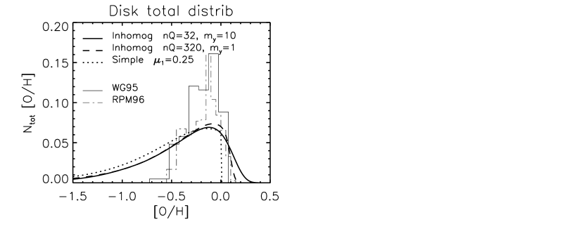
Figure 4.— MDF of Galactic disk F/G-dwarfs from Wyse & Gilmore (1995) and Rocha-Pinto & Maciel (1996). Analytic, inhomogeneous models are shown for $n=40,\ Q=0.8,\ m_{y}=10\rm\,M_{\odot}$ (solid line) and $n=400,\ Q=0.8,\ m_{y}=1\rm\,M_{\odot}$ (dashed line). The dotted curve shows the Simple Model for $z_{1}=\rm\,Z_{\odot}$. All models use $\mu_{1}=0.25$.

Figure 4 shows histograms of the empirical Galactic disk G-dwarf MDF for stars in solar neighborhood, with [Fe/H] converted to [O/H] as before. The solid curve shows the analytic inhomogeneous model for $nQ=32,\ m_{y}=10\rm\,M_{\odot}$; the dashed line shows a model with a lower yield $m_{y}=1\rm\,M_{\odot}$, which is thereby 10 times more evolved for the given mean metallicity. Finally, the dotted line shows the Simple model for $z_{1}=\rm\,Z_{\odot}$. All models take $\mu_{1}=0.25$.

The Simple model deviates most strongly from the data, illustrating the “G-dwarf Problem.” Although the inhomogeneous models do not solve the Problem, their MDFs are slightly more peaked, thus more similar to the data. Note also that Rocha-Pinto & Maciel (1996) truncated their derived distribution below an effective [O/H] $<-0.6$. The predicted [O/H] FWHM dispersions in the present-day, instantaneous MDF are 0.27 and 0.08 dex for the models with $nQ=32$ and 320, respectively. These values can be compared to the present-day observed dispersion in the solar neighborhood evidenced, for example, by the well-known –0.3 dex deviation of the Orion nebula from solar metallicity.

In summary, I present a rudimentary, one-zone model which considers overlapping areas of contamination with no mixing. This model thus represents a limiting case opposite to the homogeneous Simple model. An under-appreciated point is that the filling factor $Q$ of contamination is as important as the number of star-forming generations $n$. The product $nQ$ therefore constitutes a single parameter that describes a system’s evolutionary state. $Q$ and $n$ may be independent, and are roughly associated with the global star formation efficiency and age, respectively. Thus a system with low $Q$ can result in a present-day metal-poor ISM, but having old stars (e.g., I Zw 18); and a high $Q$ can yield an old, and simultaneously, metal-rich population (e.g., the Galactic bulge). By varying only the parameter $nQ$, the model can remarkably match both the Galactic halo and bulge metallicity distributions, and slightly improve the disk G-dwarf Problem. As expected, relatively unevolved systems are sensitive to the parent $f(z)$. For example, the high-metallicity tail of the Galactic halo MDF is consistent with a power-law $f(z)$. However, evolved systems are independent of $f(z)$ and show progressively decreasing dispersions. Further development of this inhomogeneous model, and investigation of additional empirical constraints, are currently underway.

References

- (1) Edmunds, M. G., 1975, ApSS, 32, 483
- (2) Ibata, R. A. & Gilmore, G., 1995, MNRAS, 275, 605
- (3) Laird, J. B., Rupen, M. P., Carney, B. W., & Latham, D., 1988, AJ, 96, 1908
- (4) Malinie, G., Hartmann, D. H., Clayton, D. D., & Mathews, G. J., 1993, ApJ, 413, 633
- (5) Oey, M. S. & Clarke, C. J. 1997, MNRAS, 289, 570
- (6) Oey, M. S. & Clarke, C. J. 1998, AJ, 115, 1543
- (7) Pagel, B. E. J., 1989, in Evolutionary Phenomena in Galaxies, J. E. Beckman & B. E. J. Pagel (eds.), (Cambridge: Cambridge U. Press), 201
- (8) Pagel, B. E. J. & Patchett, B. E., 1975, MNRAS, 172, 13
- (9) Rocha-Pinto, H. J. & Maciel, W. J., MNRAS, 279, 882
- (10) Roy, J.-R. & Kunth, D., 1995, AA, 294, 432
- (11) Salpeter, E. E., 1955, ApJ, 121, 161
- (12) Schmidt, M., 1963, ApJ, 137, 758
- (13) Searle, L., 1977, in The Evolution of Galaxies and Stellar Populations, B. M. Tinsley & R. B. Larson, (eds.), (New Haven: Yale Univ. Obs.), 219
- (14) Tinsley, B. M., 1975, 197, 159
- (15) Tinsley, B. M., 1980, Fund. Cosmic Phys., 5, 287
- (16) van den Hoek, L. B. & de Jong, T., 1997, AA, 318, 231
- (17) Woosley, S. E. & Weaver, T. A., 1995, ApJS, 101, 181
- (18) Wyse, R. F. G., 1995, in Stellar Populations, P. C. van der Kruit & G. Gilmore, (eds.), IAU Symp. 164, (Dordrecht: Kluwer), 133
- (19) Wyse, R. F. G. & Gilmore, G., AJ, 1995, 110, 2771