On the Association of Gamma–ray Bursts with Massive Stars: Implications for Number Counts and Lensing Statistics

Abstract

Recent evidence appears to link gamma–ray bursts (GRBs) to star–forming regions in galaxies at cosmological distances. If short–lived massive stars are the progenitors of GRBs, the rate of events per unit cosmological volume should be an unbiased tracer (i.e. unaffected by dust obscuration and surface brightness limits) of the cosmic history of star formation. Here we use realistic estimates for the evolution of the stellar birthrate in galaxies to model the number counts, redshift distribution, and time–delay factors of GRBs. We present luminosity function fits to the BATSE $\log N-\log P$ relation for different redshift distributions of the bursts. Our results imply about $1-2$ GRBs every one million Type II supernovae, and a characteristic ‘isotropic–equivalent’ burst luminosity in the range $3-20\times 10^{51}\,$ergs s^-1 (for $H_{0}=65\,\,{\rm km\,s^{-1}\,Mpc^{-1}}$). We compute the rate of multiple imaging of background GRBs due to foreground mass condensations in a $\Lambda$–dominated cold dark matter cosmology, assuming that dark halos approximate singular isothermal spheres on galaxy scales and Navarro–Frenk–White profiles on group/cluster scales, and are distributed in mass according to the Press–Schechter model. We show that the expected sensivity increase of Swift relative to BATSE could result in a few strongly lensed individual bursts detected down to a photon flux of $0.1\,\,{\rm cm^{-2}\,s^{-1}}$ in a 3–year survey. Because of the partial sky coverage, however, it is unlikely that the Swift satellite will observe recurrent events (lensed pairs).

1. Introduction

The Burst And Transient Source Experiment (BATSE) on the Compton Gamma Ray Observatory (CGRO) has detected thousands of gamma–ray bursts (GRBs) since 1991 (Paciesas et al. 1999). The distribution of BATSE bursts on the sky is isotropic, while the intensity distribution shows a clear deficiency of faint events relative to a uniform population of sources in Euclidean space (Meegan et al. 1992). Both these results provided the first clear indication for a cosmological origin of GRBs. The discovery of X–ray (Costa et al. 1997) and optical (van Paradijis et al. 1997) afterglows has permitted to firmly establish the cosmological nature of these events.

From a theoretical perspective, the physical origin of GRBs is still uncertain. Few known phenomena can release a suitable amount of energy to trigger such a powerful event, and most models associate GRBs either with merging neutron stars or with the death of massive stars. Recent observations have provided some evidence that GRBs are related to star forming regions (Paczyński 1998; Fruchter et al. 1999), and perhaps to some type of supernova explosion (Galama et al. 1998). If the violent death of massive stars (whose lifetimes are much shorter than the expansion timescale at the redshifts of interest) is somehow at the origin of the GRB phenomenon, then the rate of events per unit cosmological volume should be an unbiased tracer – unaffected by dust obscuration and surface brightness limits – of the global star formation history of the universe. It has been pointed out by many authors (Lamb & Reichart 2000; Blain & Natarajan 2000; Totani 1997, 1999; Krumholz, Thorsett, & Harrison 1999; Lloyd & Petrosian 1999; Wijers et al. 1998; Sahu et al. 1997) that standard statistical analyses of GRBs and their afterglows could then be used to derive additional constraints on the evolution of the stellar birthrate (SFR), and to gain further insight on the nature of these events.

In this paper we study the expected cosmological distribution of GRBs in the massive star progenitor scenario, identify some uncertanties in the data and in their interpretation, and discuss future observations for addressing them. We show that the brightness distribution of the BATSE bursts can be well reproduced by assuming a proportionality between the GRB rate density and observationally–based SFR estimates, once the standard candle hypothesis is relaxed (cf. Totani 1999). By itself, the bursts number–flux relation cannot discriminate between different plausible star formation histories (see Krumholz et al. 1998) since, given a SFR and assuming a functional form for the intrinsic luminosity function of GRBs, the values of free parameters can always be optimized to reproduce the observed number counts. On the other hand, quantities which reflect the redshift distribution of the bursts (like, e.g., the ratio between the average durations of bright and faint events) do depend on the underlying SFR and could be used as discriminants. With this problem in mind we also reassess the detectability of multiply–imaged GRBs due to the strong lensing effect of foreground mass concentrations (Paczyński 1986; Mao 1992). Events associated with galaxy (cluster) lenses will produce images with typical angular separations of a few ($\sim 20$) arcseconds and time delays of the order of weeks or months (years). Multiply–imaged bursts cannot be spatially resolved by present–day gamma–ray detectors and will appear as ‘mirror’ or recurrent events – same location on the sky, identical spectra and light curves – at different times and with different intensities. While a number of strongly lensed individual bursts could be detected by Swift, the restricted sky coverage makes the probability of observing a lensed pair rather small.

2. log $N$–log $P$ distribution

The photon flux (in units of $\,{\rm cm^{-2}\,s^{-1}}$) observed at Earth in the energy band $E_{\rm min}<E<E_{\rm max}$ and emitted by an isotropically radiating source at redshift $z$ is

$$P=\frac{\displaystyle(1+z)\int_{(1+z)E_{\rm min}}^{(1+z)E_{\rm max}}S(E)\,dE}{4\pi d^{2}_{\rm L}(z)}\;,$$ (1)

where $S(E)$ is the differential rest–frame photon luminosity of the source (in units of s${}^{-1}\,$ keV^-1), and $d_{L}(z)$ is the standard luminosity distance for a Friedmann–Robertson–Walker (FRW) metric. It is customary to define an ‘isotropic equivalent’ burst luminosity in the energy band 30–2000 keV as $L=\int_{30\,{\rm keV}}^{2000\,{\rm keV}}E\,S(E)\,dE$. If we denote with $\psi(L)$ the GRB luminosity function (normalized to unity), then the observed rate of bursts with observed peak fluxes in the interval $(P_{1},P_{2})$ is

$${dN\over dt}(P_{1}\leq P<P_{2})=\int_{0}^{\infty}dz\,\frac{dV(z)}{dz}\frac{R_{\rm GRB}(z)}{1+z}\int_{L(P_{1},z)}^{L(P_{2},z)}dL^{\prime}\,\psi(L^{\prime})\epsilon(P)\;,$$ (2)

where $dV/dz$ is the comoving volume element, $R_{\rm GRB}(z)$ is the comoving GRB rate density, $\epsilon(P)$ is the detector efficiency as a function of photon flux, and the factor $(1+z)^{-1}$ accounts for cosmological time dilation. If the geometry of the universe is FRW on large scales, then

$${dV\over dz}={c\over H_{0}}\frac{\Delta\Omega_{s}d_{L}^{2}(z)}{(1+z)^{2}[\Omega_{M}(1+z)^{3}+\Omega_{K}(1+z)^{2}+\Omega_{\Lambda}]^{1/2}},$$ (3)

where $\Delta\Omega_{s}$ is the solid angle covered on the sky by the survey, and $\Omega_{K}=1-\Omega_{M}-\Omega_{\Lambda}$ is the curvature contribution to the present density parameter. Unless otherwise stated, we shall assume in the following a vacuum–dominated cosmology with density parameters $\Omega_{M}=0.3$ and $\Omega_{\Lambda}=0.7$, and a Hubble constant $H_{0}=65\,h_{65}\,{\rm km\,s^{-1}\,Mpc^{-1}}$.

3. Star formation history

Our starting hypothesis is that the rate of GRBs traces the global star formation history of the universe, $R_{\rm GRB}(z)\propto R_{\rm SF}(z)\propto R_{\rm SN}(z)$, with $R_{\rm SF}$ and $R_{\rm SN}$ the comoving rate densities of star formation and core–collapse (Type II) supernovae, respectively. The constant of proportionality, $k\equiv R_{\rm SN}/R_{\rm GRB}$, is a free–parameter of the model. Popular scenarios for GRBs include merging neutron stars (Paczyński 1986) or the formation of black holes in supernova–like events (‘collapsars’, MacFadyen & Woosley 1999). The key idea here is to assume that GRBs are produced by stellar systems which evolve rapidly – by cosmological standards – from their formation to the explosion epoch. This would not be true at high redshift in the case of coalescing neutron stars, which have a median merger time of 100 Myr according to the recent population synthesis study of Bloom, Sigurdsson, & Pols (1999).

A number of workers have modelled the expected evolution of the cosmic SFR with redshift. Most have followed a similar route to that employed by Madau et al. (1996), who based their estimates on the observed (rest–frame) UV luminosity density of the galaxy population as a whole. Using various diagnostics, the cosmic SFR can now be traced to $z\approx 4$, although some details remain controversial. We use here three different parameterizations (shown in Figure 1) of the global star formation rate per unit comoving volume in an Einstein–de Sitter universe (EdS). The first (hereafter SF1) is taken from Madau & Pozzetti (2000):

$$R_{\rm SF1}(z)=0.3\,h_{65}\,\frac{\displaystyle{\exp(3.4z)}}{\displaystyle{\exp(3.8z)+45}}\,{\rm M_{\odot}\,yr^{-1}\,Mpc^{-3}}\;.$$ (4)

This star formation history matches most measured UV–continuum and H$\alpha$ luminosity densities, and includes an upward correction for dust reddening of $A_{1500}=1.2$ mag. The SFR increases rapidly between $z=0$ and $z=1$, peaks between $z=1$ and 2, and gently declines at higher redshifts. Because of the uncertainties associated with the incompleteness of the data sets and the amount of dust extinction at early epochs, we consider a second scenario in which the SFR remains instead roughly constant at $z\mathrel{\hbox to0.0pt{\lower 3.0pt\hbox{$\mathchar 536\relax$}\hss}\raise 2.0pt\hbox{$\mathchar 318\relax$}}2$ (Steidel et al. 1999),

$$R_{\rm SF2}(z)=0.15\,h_{65}\,\frac{\displaystyle{\exp(3.4z)}}{\displaystyle{\exp(3.4z)+22}}\,{\rm M_{\odot}\,yr^{-1}\,Mpc^{-3}}$$ (5)

(SF2). Some recent studies have suggested that the evolution of the SFR up to $z\approx 1$ may have been overestimated (e.g. Cowie, Songaila, & Barger 1999), while the rates at high–$z$ may have been severely underestimated due to large amounts of dust extinction (e.g. Blain et al. 1999). We then consider a third SFR,

$$R_{\rm SF3}(z)=0.2\,h_{65}\,\frac{\displaystyle{\exp(3.05z-0.4)}}{\displaystyle{\exp(2.93z)+15}}\,{\rm M_{\odot}\,yr^{-1}\,Mpc^{-3}}$$ (6)

(SF3), with more star formation at early epochs. In every case we adopt a Salpeter initial mass function (IMF) – assumed to remain constant with time – with a lower cutoff around $0.5\,M_{\odot}$ (Madau & Pozzetti 2000), consistent with observations of M subdwarf disk stars (Gould, Bahcall, & Flynn 1996). A constant multiplicative factor of 1.67 will convert the SFR to a Salpeter IMF with a cutoff of $0.1\,M_{\odot}$. To include the effect of a $\Lambda$–dominated cosmology we have computed the difference in luminosity density between an EdS and a $\Lambda$ universe, and applied this correction to the SFR above (see Appendix A for details). Assuming that all stars with masses $M>8\,{\rm M}_{\odot}$ explode as core–collapse supernovae (SNe), the SN II rate density $R_{\rm SN}(z)$ can then be estimated by multiplying the selected SFR by the coefficient

$${\int_{8}^{125}dm\,\phi(m)\over\int_{0}^{125}dm\,m\,\phi(m)}=0.0122\,{\rm M}_{\odot}^{-1}\;,$$ (7)

where $\phi(m)$ is the IMF and $m$ the stellar mass in solar units. The resulting rates agree within the errors with the locally observed value of $R_{\rm SN}=(1.1\pm 0.4)\times 10^{-4}\,h_{65}^{3}\,{\rm yr}^{-1}\,{\rm Mpc}^{-3}$ (e.g. Madau, della Valle, & Panagia 1998 and references therein).

4. Luminosity function

The observed fluxes from GRBs with secure redshifts rule out the classical standard candle hypothesis (see Table 1 of Lamb & Reichart 2000 and references therein): the inferred ‘isotropic–equivalent’ photon luminosities at peak vary by about a factor of 50, with a mean value of $3.8\,h_{65}^{-2}\times 10^{58}\,{\rm s}^{-1}$. The data are too sparse, however, for an empirical determination of the burst luminosity function, $\psi(L)$. To model the number counts we then simply assume that the burst luminosity distribution does not evolve with redshift and adopt a simple functional form for $\psi(L)$,

$$\psi(L)=C\,\left(\frac{L}{L_{0}}\right)^{\gamma}\exp\left(-\frac{L_{0}}{L}\right),$$ (8)

where $L$ denotes the peak luminosity in the 30–2000 keV energy range (rest–frame), $\gamma$ is the asymptotic slope at the bright end, $L_{0}$ marks a characteristic cutoff scale, and the constant $C=[L_{0}\Gamma(-\gamma-1)]^{-1}$ (for $\gamma<-1$) ensures a proper normalization $\int_{0}^{\infty}\psi(L)dL=1$.

5. Photon spectrum

To describe the typical burst spectrum we adopt the functional form empirically proposed by Band et al. (1993):

$$S(E)=A\times\left\{\begin{array}[]{ll}\displaystyle{\left(\frac{E}{100\,{\rm keV}}\right)^{\alpha}\exp\left[\frac{E(\beta-\alpha)}{E_{b}}\right]}&\textrm{if $E<E_{b}$}\;;\\ \displaystyle{\left(\frac{E_{b}}{100\,{\rm keV}}\right)^{\alpha-\beta}\exp{(\beta-\alpha)}\left(\frac{E}{100\,{\rm keV}}\right)^{\beta}}&\textrm{if $E\geq E_{b}$}\;.\end{array}\right.$$ (9)

For simplicity, the low and high energy spectral indices, $\alpha$ and $\beta$, have been assigned the values of $-1$ and $-2.25$, respectively, for all bursts. These are the mean values recently measured by Preece et al. (2000) for a large collection of bright BATSE events. The assumed characteristic energy of the spectral break is $E_{b}=511$ keV. Note that the method introduced by Fenimore & Bloom (1995) to account for the spectral diversity of bursts by averaging the number counts over the spectral catalog by Band et al. (1993) cannot be rigorously applied when the standard candle hypothesis is relaxed. We have checked, a posteriori, the stability of our results with respect to small variations of the spectral parameters. This issue is briefly discussed in the next session.

6. Comparison with the data

Table 1Best–fitting parameters for the $\log N-\log P$ relation.

Model	$\gamma$	$L_{0}(10^{51}h^{-2}_{65}{\rm erg\,s}^{-1})$	$k_{\rm B}(10^{5}h^{-2}_{65})$	$\chi^{2}_{\rm B}$	$k_{\rm P}(10^{5}h^{-2}_{65})$	$\chi^{2}_{\rm P}$
SF1	$-2.5\pm 0.2$	$3.2^{+1.0}_{-0.7}$	$4.4\pm 0.2$	$18.5$	$1.82^{+0.17}_{-0.14}$	$6.26$
SF2	$-2.9^{+0.4}_{-0.6}$	$7^{+4}_{-2}$	$6.0^{+0.4}_{-0.3}$	$20.9$	$2.17^{+0.20}_{-0.17}$	$5.69$
SF3	$-3.7^{+0.8}_{-2.2}$	$17^{+19}_{-8}$	$8.2^{+0.4}_{-0.5}$	$23.2$	$2.82^{+0.26}_{-0.22}$	$5.70$

To calibrate and test our models against the observed number counts we have used the off–line BATSE sample of Kommers et al. (2000), which includes 1998 archival BATSE (“triggered” plus “non–triggered”) bursts in the energy band 50–300 keV. The efficiency of this off–line search is well–described by the function $\epsilon(P)=0.5[(1+{\rm erf}(-4.801+29.868P)]$ (Kommers et al. 2000).

We have optimized the value of our three free parameters, $k,\gamma$ and $L_{0}$, by $\chi^{2}$ minimization over 25 peak flux intervals (see Table 2 in Kommers et al. 2000). In Figure 2 we show the best–fitting results for the three different star formation histories considered. The observed number counts have been converted into rates per unit time per unit solid angle by estimating the effective live time of the searches and their field of view following Kommers et al. (2000). Assuming a normal distribution for the errors, we can relate confidence levels to value intervals for the free parameters. Table 1 gives the chi–square of the best–fitting models, $\chi^{2}_{\rm B}$, the ranges corresponding to the $68\%$ confidence level for the parameters that determine the luminosity function ($\gamma$ and $L_{0}$), and the expected number of core–collapse supernovae per BATSE burst, $k_{\rm B}$.

The overall quality of the best–fit decreases when the star formation rate at high redshift is increased, i.e. as the models start predicting too many bursts to be consistent with the faintest off–line BATSE counts: the minimum $\chi^{2}$ per degree of freedom is $18.5/22=0.84$ for $R_{\rm SF1}$, $20.9/22=0.95$ for $R_{\rm SR2}$, and $23.2/22=1.05$ for $R_{\rm SF3}$.

Table 2Moments of the best–fitting luminosity functions (all in units of $10^{51}h^{-2}_{65}{\rm erg\,s}^{-1}$).

Model	$L_{5}$	$L_{95}$	$\langle L\rangle$	$L_{50}$	$L_{+}$
SF1	$0.82$	$18.19$	$6.40$	$2.71$	$1.28$
SF2	$1.57$	$22.78$	$8.00$	$4.56$	$2.48$
SF3	$2.82$	$24.71$	$9.71$	$6.95$	$4.46$

Strong covariance of $\gamma$ and $L_{0}$ is observed in the region of parameter space surrounding the best–fitting values. When the slope of the high–luminosity tail of the $\psi(L)$ is increased, one has to correspondingly raise the value of the cutoff luminosity to prevent a strong $\chi^{2}$ increment: this means that our models need the presence of relatively high–luminosity events to reproduce the data. Luminosity intervals corresponding to $90\%$ of the bursts (obtained excluding the $5\%$ tails on both sides) are given in Table 2. The average ($\langle L\rangle$), median ($L_{50}$), and mode ($L_{+}$) of the distributions are also given . The derived rate of GRBs at the present epoch ranges from $(0.181\pm 0.008)\,h_{65}^{-1}\,{\rm yr}^{-1}\,{\rm Gpc}^{-3}$ (SF1) down to $(0.133^{+0.006}_{-0.009})\,h_{65}^{-1}\,{\rm yr}^{-1}\,{\rm Gpc}^{-3}$ (SF2) and $(0.125^{+0.008}_{-0.006})\,h_{65}^{-1}\,{\rm yr}^{-1}\,{\rm Gpc}^{-3}$ (SF3). The best–fit values for $\gamma$ and $L_{0}$ are found to be rather insensitive to $20\%$ variations in the spectral parameters $\alpha$ and $E_{0}$. The cutoff scale of the luminosity function, however, depends more sensitively on the assumed value of the high–energy spectral index $\beta$ (this is especially true for $\beta>-2.25$). For example, for SF1 and $\beta=-2.0$, the best–fitting parameters become $L_{0}=3.7^{+1.0}_{-0.8}$ and $\gamma=-2.5\pm 0.2$.

It is of interest to compare the properties of the luminosity functions that provide the best–fit for each star formation rate. As expected, to balance the effect of cosmic expansion, the typical burst luminosity increases in models with larger amounts of star formation at early epochs (see Table 2). Moreover, changing from SF1 to SF3, the luminosity function broadens, becoming less and less peaked around $L_{+}$, while the slope of the luminosity function in the range $L_{+}\mathrel{\hbox to0.0pt{\lower 3.0pt\hbox{$\mathchar 536\relax$}\hss}\raise 2.0pt\hbox{$\mathchar 316\relax$}}L\mathrel{\hbox to0.0pt{\lower 3.0pt\hbox{$\mathchar 536\relax$}\hss}\raise 2.0pt\hbox{$\mathchar 316\relax$}}L_{95}$, $\gamma_{\rm eff}$, remains the same in all the models, $\gamma_{\rm eff}\sim 2.3$. An increase in the amount of star–formation at high redshifts requires a steeper high–luminosity tail of $\psi(L)$. Regrettably, since the number of GRBs with known redshift is very small, it is not yet possible to use observational data to discriminate among different luminosity functions (see below, however, for a comparison between the redshift distributions of bursts predicted by our models as a function of measured peak flux, and the available data).

Table 3Average redshifts and time–delay factors.

Model	$\langle z\rangle_{\rm b}$	$\langle z\rangle_{\rm i}$	$\langle z\rangle_{\rm f}$	$\langle z\rangle_{\rm t}$	$\langle z\rangle_{\rm Nb}$	$\langle z\rangle_{\rm Nd}$	$\displaystyle{\frac{\langle 1+z\rangle_{\rm Nd}}{\langle 1+z\rangle_{\rm Nb}}}$	$\langle z\rangle_{\rm Nb^{\prime}}$	$\langle z\rangle_{\rm Nd^{\prime}}$	$\displaystyle{\frac{\langle 1+z\rangle_{\rm Nd^{\prime}}}{\langle 1+z\rangle_{\rm Nb^{\prime}}}}$
SF1	$0.94$	$1.45$	$2.29$	$1.67$	$0.99$	$1.59$	$1.30$	$0.90$	$1.58$	$1.36$
SF2	$0.92$	$1.72$	$3.10$	$2.08$	$1.00$	$1.94$	$1.47$	$0.85$	$1.92$	$1.57$
SF3	$0.85$	$1.89$	$3.71$	$2.37$	$0.96$	$2.19$	$1.63$	$0.77$	$2.16$	$1.79$

To test our models against observations of very bright and rare bursts we have also used the number counts accumulated by the Pioneer Venus Orbiter (PVO) at $20<P<1000\,\,{\rm cm^{-2}\,s^{-1}}$ in the 100–500 keV band (see Table 2 in Fenimore & Bloom 1995). Since no threshold effects are expected in the PVO detection of such bright events, we set $\epsilon(P)=1$ in equation (2) for the counts. By combining PVO and BATSE data we should be able to test our models over about 3.5 orders of magnitudes in peak flux. We find that, while our best–fitting models for the BATSE counts have the right shape to accurately describe the PVO rates (roughly a $3/2$ power–law), the predicted counts need to be multiplied by a factor of $\sim 2.5-3$ to have the right normalization (see Figure 2). To better quantify this discrepancy, we have minimized the chi–square function using only PVO data (divided in 6 bins as in Fenimore & Bloom 1995), and allowing just the parameter $k$ to vary, while assigning to $\gamma$ and $L_{0}$ the values given in Table 1. The resulting minimum chi–square, $\chi^{2}_{\rm P}$, and the corresponding normalization constant of the GRB rate, $k_{\rm P}$, are shown in Table 1. It is possible that the PVO and off–line BATSE catalogues, using different selection criteria, may not form a homogeneous burst sample.   The PVO catalogue does not report the trigger time–scale for burst detection, and each light curve has been analyzed a posteriori to select only events above the detection threshold on timescales of either 0.25 s or 1 s. Kommers et al. (2000) have included only events detected on a timescale of 1.024 s: short–duration bursts may then be under–represented in the off–line BATSE sample. Alternatively, the discrepancy could be explained with the existence of a local (bright) population of GRBs. In the following we will only include long–duration bursts in our analysis and use models calibrated against archival BATSE data.

In Figure 3, the expected redshift distribution of bursts, $d/dz(dN/dt)$ (with $dN/dt$ defined in eq. 2), is plotted as a function of redshift for a number of selected luminosity intervals (the efficiency of BATSE off–line search is assumed), and two different star formation histories: SF1 (upper panels) and SF3 (lower panels). Bright events ($P\geq 1\,{\rm cm^{-2}\,s^{-1}}$) are depicted in the left panels, faint bursts on the right. The peak flux intervals used by Kommers et al. (2000) (approximately evenly spaced in $\log P$) which contain at least one GRB with known redshift are considered. A similar analysis for the faint bursts ($P<1\,{\rm cm^{-2}\,s^{-1}}$) is performed in the right panels. In this case, we also plot the redshift distribution of the sources corresponding to two luminosity intervals in which no afterglow redshifts have been determined. The redshifts of bursts with known optical counterparts (see Table 1 of Lamb & Reichart 2000), including GRB000301C (Smith, Hurley, & Kline 2000; Castro et al. 2000) are also shown as filled points on the curve corresponding to their observed brightness. We do not include GRB980425 in this analysis, since its association with SN 1998 bw (a Type Ic at $z=0.0085$) is uncertain (Pian et al. 2000). It might well be the case that GRB980425 is representative of a special class of GRBs (e.g. Bloom et al. 1998).

Note that, barring selection effects, model SF1 can reasonably account for all but the highest observed redshift ($z=3.418$ for GRB971214), which has a low a priori probability in all three models (cf. Schmidt 1999). The detection of relatively faint bursts at $z\sim 1$ (like GRB970508 and GRB980613) appears improbable in model SF3. Table 3 lists the expected average redshift of GRBs observed in three selected flux ranges: a bright sample ($7.94<P<20\,\,{\rm cm^{-2}\,s^{-1}}$, subscript $b$), an intermediate sample ($1.0<P<2.26\,\,{\rm cm^{-2}\,s^{-1}}$, subscript $i$), and a faint sample ($0.18<P<0.20\,\,{\rm cm^{-2}\,s^{-1}}$, subscript $f$). The entire interval $0.18<P<20\,\,{\rm cm^{-2}\,s^{-1}}$ is also considered (subscript $t$). The redshift distribution of GRBs has another direct observational consequence: because of cosmic expansion, faint bursts will have longer durations than bright ones, on the average. This time dilation effect is proportional to $1+z$. Even though observational results are still controversial, a cosmological time dilation factor of about 2 between dim and bright bursts is widely accepted for the long duration events (Norris et al. 1994, 1995; Norris 1996). The average redshifts of the bursts lying in the peak flux intervals considered by Norris et al. (1995) are also shown in Table 3. The quantities $\langle z\rangle_{\rm Nb}$ and $\langle z\rangle_{\rm Nd}$ refer, respectively, to their bright ($4.21\leq P\leq 58.28\,\,{\rm cm^{-2}\,s^{-1}}$) and combined dim + dimmest ($0.33\leq P\leq 2.82\,\,{\rm cm^{-2}\,s^{-1}}$) samples (see Table 1 in Horack, Mallozzi & Koshut 1996). Since, for both classes of GRBs, the peak flux distribution of the dataset used in the analysis of Norris et al. (1995) is strongly peaked around the mean value, we repeated our calculations considering smaller $P$ intervals. The quantities $\langle z\rangle_{\rm Nb^{\prime}}$ and $\langle z\rangle_{\rm Nd^{\prime}}$ are, in fact, performed over the ranges of peak flux corresponding to $\langle P\rangle\pm 2\sigma_{\langle P\rangle}$ (i.e. $12.34\leq P\leq 20.06\,\,{\rm cm^{-2}\,s^{-1}}$ for the bright sample, and $0.72\leq P\leq 0.84\,\,{\rm cm^{-2}\,s^{-1}}$ for the faint one), with $\sigma_{\langle P\rangle}$ the standard deviation of the mean. The time dilation estimates of $\sim 2.25$ (Norris et al. 1995) and $\sim 1.75$ (Norris 1995) appear to favor scenarios in which the SFR does not decrease at high–redshift. On the other hand, SF1 is slightly preferred to the other cosmic star formation histories by the $\,\log N-\log P$ analysis of the BATSE data (see the $\chi^{2}_{\rm B}$ values in Table 1). A recent search for non–triggered GRBs in the BATSE records (Stern et al. 2000), however, has detected many more faint bursts than the analysis by Kommers et al. (2000). The ratio between the estimated number counts can be as high as a factor of $\sim 2$ at $P=0.2\,{\rm cm^{-2}\,s^{-1}}$. If confirmed, a large number of faint counts would probably favor scenarios in which the star–formation rate does not substantially decrease at $z\mathrel{\hbox to0.0pt{\lower 3.0pt\hbox{$\mathchar 536\relax$}\hss}\raise 2.0pt\hbox{$\mathchar 318\relax$}}3-4$.

7. Gravitational lensing of GRBs

In the observable (clumpy) universe, gravitational lensing will magnify and demagnify high redshift GRBs relative to the predictions of ideal (homogeneous) reference cosmological models. A burst that goes off within the Einstein ring of a foreground mass concentration may generate multiple images at different positions on the sky. The magnitude and frequency of the effect depend on the redshift distribution of the sources, the abundance and the clustering properties of virialized clumps, the mass distribution within individual lenses, and the underlying world model. Events associated with galaxy (cluster) lenses will produce images with typical angular separations of a few ($\sim 20$) arcseconds, smaller than the presently achievable $\gamma$–ray instrumental resolution. On the other hand, GRBs are transient phenomena with durations ranging from a fraction of a second to several hundreds seconds, while the typical time delay between multiple images is of the order of weeks in the case of galaxy lensing, and years for lensing by a foreground cluster. Mirror images of the same burst will then appear as separate events with overlapping positional error boxes, identical time histories, and intensities that differ only by a scale factor. In principle, the detection of two or more images satisfying these three conditions should pinpoint a good candidate for a lensed GRB. However, temporal variation of the background signal and the presence of noise in observed light curves can make this task estremely difficult (Wambsganss 1993), and special statistical methods devised to minimize the effect of the noise must be adopted for light curve comparison (e.g. Nowak & Grossman 1994).

In this section we estimate the number of multiply–imaged GRBs expected as a function of the limiting sensitivity of the survey, and for the different star formation histories discussed in § 3. We improve upon previous calculations of GRB lensing by using more realistic models of the burst redshift and brightness distributions, and of the foreground mass concentrations. Following our previous study on high–$z$ supernovae (Porciani & Madau 2000), we assume that lensing events are caused by intervening dark matter halos which approximate singular isothermal spheres on galaxy scales and Navarro–Frenk–White (Navarro, Frenk, & White 1997; hereafter NFW) profiles on group/cluster scales, and are distributed in mass according to the Press–Schechter (Press & Schechter 1974; hereafter PS) theory. This model for the lens population provides a good fit to the data on QSO image separations lensing, and may originate in a scheme which includes the dissipation and cooling of the baryonic protogalactic component and the radial re–distribution of the collisionless dark matter as a consequence of baryonic infall (e.g. Keeton 1998). The strong lensing optical depth for a light–beam emitted by a point source at redshift $z_{s}$ is (Turner, Ostriker, & Gott 1984)

$$\tau(z_{s})=\int_{0}^{z_{s}}dz(1+z)^{3}\frac{dl}{dz}\int_{0}^{\infty}dM\,\Sigma(M,z,z_{s})n(M,z)\;,$$ (10)

where $dl/dz=cH_{0}^{-1}(1+z)^{-1}[\Omega_{M}(1+z)^{3}+\Omega_{K}(1+z)^{2}+\Omega_{\Lambda}]^{-1/2}$ is the cosmological line element, $\Sigma(M,z,z_{s})$ is the lensing cross section as measured on the lens–plane, and $n(M,z)$ the comoving differential distribution of halos with mass $M$ at redshift $z$. Equation (10) assumes that each bundle of light rays encounters only one lens, the lens population is randomly distributed, and the resulting $\tau\ll 1$. The mass distribution in a single lens and the geometry of the source–lens–observer system completely determine $\Sigma(M,z,z_{s})$. For a singular isothermal sphere (SIS) with one–dimensional velocity dispersion $\sigma_{v}$, the strong lensing cross section is

$$\Sigma_{\rm SIS}(\sigma_{v},z_{s},z_{l})=16\pi^{3}\left(\frac{\sigma_{v}}{c}\right)^{4}\left(\frac{D_{l}D_{ls}}{D_{s}}\right)^{2}\;,$$ (11)

where $D_{l},D_{s},$ and $D_{ls}$ are the angular diameter distances between the observer–lens, the observer–source, and the lens–source systems. According to the PS theory, the differential comoving number density of dark halos with mass $M$ at redshift $z$ is given by

$$n(M,z)=\frac{1}{\sqrt{2\pi}}\frac{\rho_{0}}{M}\frac{\delta_{c}(z)}{\sigma_{M}^{3}}\exp\left[-\frac{\delta_{c}^{2}(z)}{2\sigma_{M}^{2}}\right]\left|\frac{d\sigma_{M}^{2}}{dM}\right|\;,$$ (12)

where $\rho_{0}$ is the present mean density of the universe. The halo abundance is then fully determined by the redshift–dependent critical overdensity $\delta_{c}$ (e.g. Eke, Cole, & Frenk 1996) and by the linearly extrapolated (to $z=0$) variance of the mass–density field smoothed on the scale $M$, $\sigma_{M}^{2}$. The latter is computed assuming a scale–invariant power–spectrum of primordial density fluctuations with spectral index $n_{\rm p}=0.96$ and the transfer function for CDM given in Bardeen et al. (1986). The amplitude of density perturbations is fixed by requiring the (present–day, linearly extrapolated) rms mass fluctuation in a $8\;h^{-1}$ Mpc sphere to be $\sigma_{8}=0.87$.

Assuming that every halo virializes to form a (truncated) singular isothermal sphere of velocity dispersion $\sigma_{v}$, mass conservation implies

$$\sigma_{v}(M,z)=\frac{1}{2}H_{0}\left(\frac{3M}{4\pi\rho_{0}}\right)^{1/3}\,\Omega_{M}^{1/3}\Delta^{1/6}\left[\frac{\Omega_{M}}{\Omega(z)}\right]^{1/6}(1+z)^{1/2}\;,$$ (13)

where $\Omega(z)=\Omega_{M}(1+z)^{3}/[\Omega_{M}(1+z)^{3}+\Omega_{K}(1+z)^{2}+\Omega_{\Lambda}]$. Here $z$ denotes the virialization epoch of the halo, and $\Delta(z)$ is the ratio between its actual mean density at virialization and the corresponding critical density, $\rho_{\rm crit}(z)=3H^{2}(z)/8\pi G$ (here $H(z)$ the Hubble parameter at redshift $z$, and $G$ the gravitational constant). Equation (13) relates the PS mass function to the SIS lens profile, therefore allowing the computation of the optical depth given in equation (10). For the NFW density profile – shallower than isothermal near the halo center and steeper than isothermal in its outer regions – the lens equation must be solved numerically. With respect to a halo SIS profile containing the same total mass, a NFW lens has a smaller cross section for multiple imaging, but generates a higher magnification.

The resulting optical depths for strong lensing are plotted in Figure 4 for our reference cosmology ($\Lambda$CDM) and two other popular cold dark matter models: OCDM ($\Omega_{M}=0.3$, $\Omega_{\Lambda}=0$, $n_{\rm p}=1$, $\sigma_{8}=0.85$, and $H_{0}=70\,\,{\rm km\,s^{-1}\,Mpc^{-1}}$), and SCDM ($\Omega_{M}=1$, $\Omega_{\Lambda}=0$, $n_{\rm p}=1$, $\sigma_{8}=0.5$, and $H_{0}=50\,\,{\rm km\,s^{-1}\,Mpc^{-1}}$). In all cases the amplitude of the power spectrum has been fixed in order to reproduce the observed abundance of rich galaxy clusters in the local universe (e.g. Eke, Cole & Frenk 1996). In $\Lambda$CDM a convenient fit to the lensing optical depth is

$$\tau(z)={8.4\times 10^{-4}\over 3.1z^{-2.85}-0.39z^{-1.42}+z^{-1}+9.5\times 10^{-4}z^{1.5}},$$ (14)

to within 1% in the range $0.6<z<7$. Our analytical method is expected to be very accurate for sources at $z_{s}\leq 3$, and to slightly underestimate the optical depth for multiple lensing at higher redshift (Holz, Miller, & Quashnock 1999).

The cumulative rate of lensed GRBs can then be computed as

$${dN\over dt}=\int_{0}^{\infty}dz\,\frac{dV(z)}{dz}\frac{R_{\rm GRB}(z)}{1+z}\int_{0}^{\infty}dL\,\psi(L)\int_{\mu_{\rm min}(L,z)}^{\infty}d\mu\,{\cal P}(\mu,z)\epsilon[\mu P(L,z)]\;,$$ (15)

where $\mu_{\rm min}(L,z)$ is the minimum magnification needed to detect a source in a flux–limited survey. The above equation relates the number counts to the probability distribution of magnification, ${\cal P}(\mu,z)$, which is related to $\tau(z)$ as discussed in Porciani & Madau (2000). The detection rates for the two brightest detectable images of strongly lensed GRBs are compared with the total number counts in Figure 5. These results have been obtained by considering the different star formation histories discussed above (solid, short–dashed, and long–dashed lines refer to SF1, SF2, and SF3, respectively), and taking $\epsilon(P)=1$. The upper set of curves (which lie approximately on top of each other since we impose our models to provide the same number counts in the BATSE energy band) represents the GRB counts in absence of any lensing effects. The $\log N-\log P$ relation has a $-3/2$ slope at the bright end ($P\mathrel{\hbox to0.0pt{\lower 3.0pt\hbox{$\mathchar 536\relax$}\hss}\raise 2.0pt\hbox{$\mathchar 318\relax$}}10\,{\rm cm^{-2}\,s^{-1}}$) and progressively flattens out with decreasing limiting flux. The remaining two sets of curves show, respectively, the count–rates for the brightest and the second brigthest images of strongly lensed GRBs. Qualitatively, the shapes of these curves are similar to those of the unlensed counts. The limiting peak flux at which they flatten out, however, depends on the assumed star formation history, and decreases from SF1 to SF3 as the lensing cross–section increases with the source redshift. Note that the rates in Figure 5 are all–sky averages, and the detection of the fainter image (the last to reach the observer) does not imply that its brighter counterpart will also be observed. This is because satellite experiments generally guarantee only partial sky (and temporal) coverage and have a rapidly varying field–of–view. In this case the detection of multiple images of the same event has a much smaller probability. For a perfect detector – full sky and time coverage plus $\epsilon=1$ – our models predict the presence of a doubly–imaged event every 2557, 1886, and 1615 bursts with $P>1\,\,{\rm cm^{-2}\,s^{-1}}$ for SF1, SF2 and SF3, respectively. At fainter fluxes, $P>0.01\,\,{\rm cm^{-2}\,s^{-1}}$, recurrent events will be detected every 888, 533, and 420 bursts instead.

Marani (1998) has compared the light curves of the brightest $75\%$ events of a sample containing 1235 BATSE bursts. Her analysis revealed the absence of good lens candidates with $P>1\,\,{\rm cm^{-2}\,s^{-1}}$, a result largely expected because of the low efficiency of BATSE at detecting multiply–imaged bursts. As a consequence of Earth blockage, BATSE could only monitor $\sim 2/3$ of the sky at the same time. Moreover, the trigger was disabled during readout time and when the spacecraft was in specific locations. Depending on declination, the angular exposure (i.e. the fraction of time during which burst detection is possible in a given direction of the sky) of the 4B catalogue ranges between 0.44 and 0.6, with a mean value of 0.48 (Hakkila et al. 1998). Since the orbital period of CGRO was only $\sim 5000$ s, the BATSE efficiency for detecting a burst in a particular direction of the sky varied with a characteristic time–scale which was much shorter than the typical time–delay between lensed multiple images. In other words, the phases of the CGRO orbit at which two mirror images of a burst could be observed were practically uncorrelated: the efficiency of multiply–imaged detection is then proportional to $\epsilon(\mu_{1}P)\times\epsilon(\mu_{2}P)$, and roughly 3/4 of lensed events remained undetected. We will see in the next section that, because of the inefficient duty cycle, the probability of detecting a double burst is quite small even in a more sensitive future experiment like Swift.

8. Discussion

In a flux–limited sample, sources that are observed to be gravitationally lensed include not only the lensed objects that are intrinsically brighter than the flux limit, but also sources that are intrinsically fainter but are brought into the sample by the magnification effect Relative to the optical depth shown in Figure 4, lensed systems will then be overrepresented among GRBs of a given peak flux. We have quantified this effect from the GRBs number counts, by defining the magnification bias $B$ as the ratio between the actual flux–limited counts of lensed GRBs and the counts of lensed events that are intrinsically brighter than the flux limit,

$$B(<P)=\frac{\displaystyle{\int_{0}^{\infty}dz\,\frac{dV(z)}{dz}\frac{R_{\rm GRB}(z)}{1+z}\int_{0}^{\infty}dL\,\psi(L)\,\epsilon\int_{\mu_{\rm min}(L,z)}^{\infty}{\cal P}(\mu,z)\,d\mu}}{\displaystyle{\int_{0}^{\infty}dz\,\frac{dV(z)}{dz}\frac{R_{\rm GRB}(z)}{1+z}\int_{L(P,z)}^{\infty}dL\,\psi(L)\,\epsilon\int_{\mu_{\rm min}(L,z)}^{\infty}{\cal P}(\mu,z)\,d\mu}}\;.$$ (16)

This definition (Porciani & Madau 2000) generalizes that given in Turner, Ostriker & Gott (1984) by taking into account the redshift dependence of the lensing optical depth. The magnification bias for the two brightest images of a GRB is plotted in Figure 6 (for $\epsilon=1$). At faint fluxes, where lensing becomes a significant effect, the bias is small as a consequence of the flatness of the burst $\log N-\log P$ relation. Contrary to quasars, where the number of sources at a given flux rises steeply at the faint end, there are relatively few GRBs to be brought into the flux–limited sample by the magnification effect. The situation is different for bright bursts. In this case, the steepening of the $\log N-\log P$ relation causes a rapid increase of the magnification bias. However, as shown in Figure 5, the absolute rate of lensed events is extremely low for such luminous events.

It is interesting to use our modelling of the GRBs number counts, redshift distribution, and lensing probability to make predictions for a future space mission like the Swift Gamma Ray Burst Explorer, a multiwavelength orbiting observatory selected by NASA for launch in the 2003 . Its main instrument will be the Burst Alert Telescope (BAT) in the 10–150 keV energy range. A X–ray telescope (XRT) and an ultraviolet and optical telescope (UVUOT) complete the onboard instrumentation and will be used to study afterglows and get accurate determinations of burst locations. In Figure 7 we plot our estimates for the GRB number counts accumulated by the BAT in a 3–year survey, as a function of limiting flux $P$. These have been computed in the energy band $10-150$ keV, assuming a field of view of 2 sr and $\epsilon=1$. The expected sensitivity of the BAT should be close to $0.14\,\,{\rm cm^{-2}\,s^{-1}}$ in the fully–coded field of view ($0.2\,\,{\rm cm^{-2}\,s^{-1}}$ half–coded), assuming a flat–topped GRB of duration 2 s and an 8–sigma detection (D. Palmer, personal communication). Note that, even though the luminosity functions and the overall spatial density of bursts have been fixed to reproduce the BATSE rates, the Swift counts corresponding to SF1 and SF3 disagree by about a factor of two at both the faint and bright ends. This shows how data from BATSE and Swift could be combined to set additional constraints on the statistical properties of GRBs.

The number of lensed images that could be detected with the BAT is small. As shown in Figure 7, in a 3–year survey with $P>0.1\,\,{\rm cm^{-2}\,s^{-1}}$, Swift should detect 0.45 secondary lensed images (i.e. the second brightest images of strongly lensed events) over a total number of 525 bursts for SF1, 0.90 over 611 for SF2, and 1.34 over 760 for SF3. Even at $P>0.01\,\,{\rm cm^{-2}\,s^{-1}}$, the number of lensed images would not sensibly increase: 0.78 over 573 for SF1, 1.73 over 715 for SF2, and 2.74 over 908 for SF3. In a SCDM cosmology the numbers are typically 40% higher. In any case, since the field of view of BAT covers a small fraction of the sky, the probability of detecting a lensed pair is extremely low.

For particular configurations, lensed pairs could also be detected by combining BAT and XRT observations. The XRT will make high resolution spectroscopic observations of afterglows from the initial acquisition ($\sim 50$ s after the burst) for up to 10 hours, while spectrophotometric observations will go on for up to 4 days after the burst. Thus, if the time delay between the different components of a strongly lensed system is as small as a few days, the secondary image may be easily detected by the XRT during follow–up observations (even when too weak to trigger the BAT). For a given lensing halo, and at fixed source and lens redshifts, the time delay is anti–correlated with the magnification: smaller delays correspond to more perfect source–lens alignments and thus to larger magnifications. On the other hand, less massive deflectors will always produce relatively short delays. For example, in our $\Lambda$CDM cosmology, isolated SIS lenses at $z=0.5$, deflecting the light emitted by a point source at $z_{s}=2$ and having masses of $10^{12}$, $10^{11}$ and $10^{10}$ $M_{\odot}$, will produce maximum delays of 6.6, 1.4 and 0.3 days, respectively. Thus, the search for short–delayed images of lensed bursts could be optimized following up those bursts which are located in the vicinity of field galaxies having redshifts between 0.5 and 1. Assuming SIS+NFW lenses distributed in mass according to the PS theory, and considering a point source at $z_{s}=2$, we find that $\sim 15\%$ of the bursts which generate multiple images will have time delays smaller than 4 days. This implies that, on average, only about one lensed pair should be detected during a 3–year survey.

So far we have confined our attention to axially symmmetric lenses producing two observable images. Non axisymmetric (e.g. elliptical) potentials, however, generally produce 5 images (one of them always strongly demagnified and in practice unobservable), and this may increase the odds of a successful lensing detection. As shown by Grossman & Nowak (1994), the probability of observing two or more images out of $n$ above the detection limit follows a binomial distribution

$${\cal P}(\geq 2|n)=\sum_{i=2}^{n}\left({}^{n}_{i}\right)p^{i}(1-p)^{n-i}\;,$$ (17)

where $p$ is the probability of detecting a single image. Taking the sky coverage of Swift ($1/2\pi$) as a representative value for $p$, one gets: ${\cal P}(\geq 2|2)=0.025$, ${\cal P}(\geq 2|3)=0.068$ and ${\cal P}(\geq 2|4)=0.122$. If systems producing 4 sufficiently bright images are common, then the probability of detecting a recurrent burst is a factor of 5 higher than estimated by considering axisymmetric lenses only. For QSOs, doubly–imaged objects account roughly for one–half of all lensed systems, groups of 4 images contribute for another $30\%$ (see http://cfa–www.harvard.edu/castles/index.htm). In the case of GRBs, the magnitude of this enhancement will depend on their redshift distribution.

Appendix A. Star formation rate density in different cosmologies

The estimate for the luminosity density at redshift $z$, obtained by combining photometric and spectroscopic data of a galaxy sample, depends on the assumed underlying cosmology. In particular, it comes out proportional to the quantity $F(z|\Omega_{M},\Omega_{\Lambda},h_{65})=d_{L}^{2}(z)/(dV/dz)$. Thus,

$$R_{\rm SF}(z|\Omega_{M},\Omega_{\Lambda},h_{65})=\frac{F(z|\Omega_{M},\Omega_{\Lambda},h_{65})}{F(z|1,0,1)}R_{\rm SF}(z|1,0,1)=\frac{H(z|\Omega_{M},\Omega_{\Lambda},h_{65})}{H(z|1,0,1)}R_{\rm SF}(z|1,0,1)\;,$$

and, expliciting the dependence of the Hubble expansion rate $H$ on the cosmological parameters, we eventually get

$$R_{\rm SF}(z|\Omega_{M},\Omega_{\Lambda},h_{65})=h_{65}\frac{[\Omega_{M}(1+z)^{3}+\Omega_{K}(1+z)^{2}+\Omega_{\Lambda}]^{1/2}}{(1+z)^{3/2}}R_{\rm SF}(z|1,0,1)\;.$$

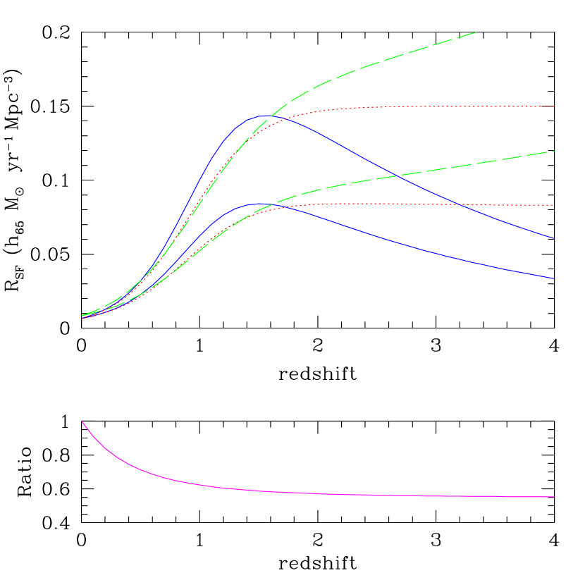
Figure 1.— Cosmic star formation history. The continuous, dotted, and dashed curves show the rate of star formation per unit comoving volume as a function of redshift, for our models SF1, SF2, and SF3, respectively. The top set of curves refers to an EdS universe, while the lower lines are for a $\Lambda$–dominated cosmology. The ratio between the two sets is shown in the small panel at the bottom.

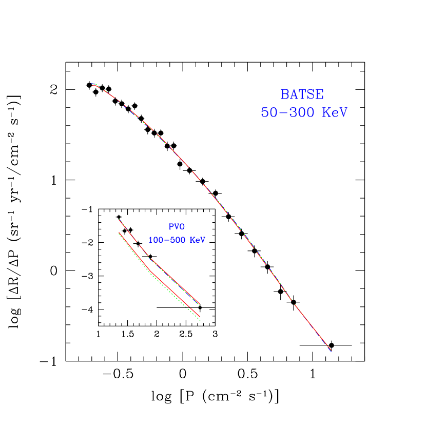
Figure 2.— Differential GRB number counts versus peak photon flux. The points and vertical error bars show the observed rates from Kommers et al. (2000) and their Poisson uncertainties (horizontal error bars denote bin sizes). The best–fit models obtained by assuming that the burst rate is proportional to SF1, SF2 and SF3 are shown with (overlapping) solid, dotted, and dashed lines, respectively. The comparison of the model results with PVO rates is depicted in the inset. In this case two sets of curves are plotted: the upper one represents the best fit to the PVO data, the lower set the extrapolation of the rates shown in the main panel.

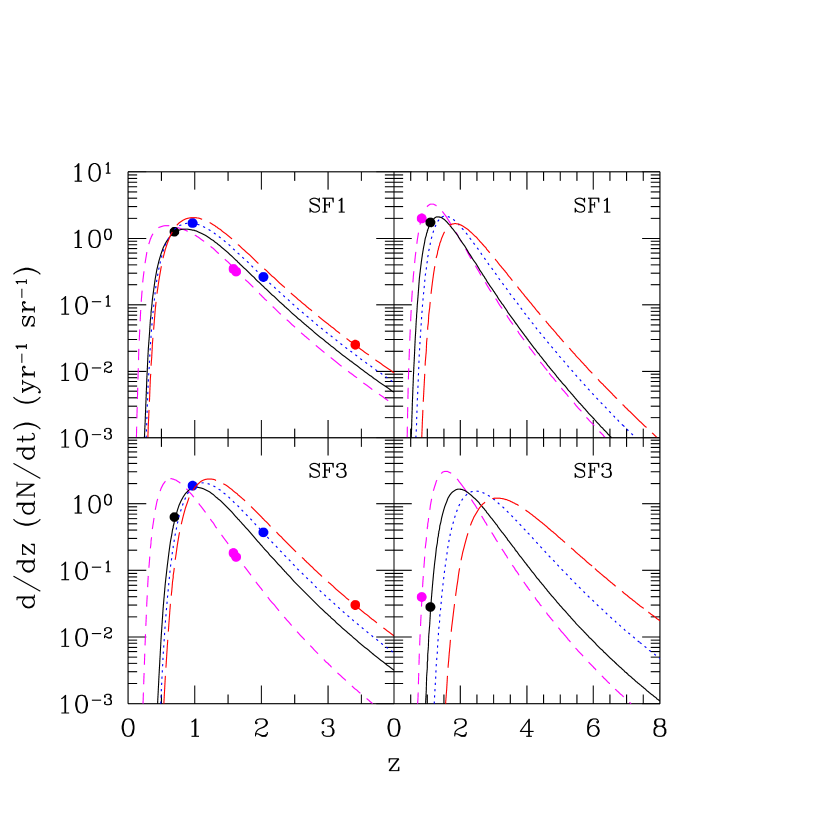
Figure 3.— Redshift distributions of the bursts detected in the off–line search by Kommers et al. (2000). In the left panels the short–dashed, solid, dotted, and long–dashed curves refer, respectively, to the peak flux ($\,{\rm cm^{-2}\,s^{-1}}$) intervals $(7.943,20.00)$, $(3.162,3.981)$, $(2.511,3.162)$, and $(1.995,2.511)$. The corresponding intervals in the right panels are $(1.000,1.259)$, $(0.569,0.639)$, $(0.320,0.359)$, and $(0.180,0.202)$. The curves in the upper (lower) panels have been derived assuming a burst rate proportional to SF1 (SF3). GRBs with known redshifts have been plotted as filled points on the curve corresponding to their observed brightness.

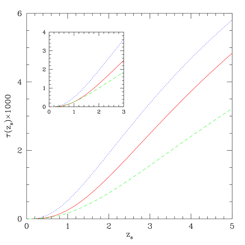
Figure 4.— Strong lensing optical depths for a point source at $z_{s}$ in three different hierarchical cosmogonies. The mass distribution of the lenses is described by the Press–Schechter theory; a lens having mass $M$ is modelled by a singular isothermal sphere for $M<3.5\times 10^{13}M_{\odot}$, and by a NFW profile otherwise. Solid line: $\Lambda$CDM. Dashed line: OCDM. Dotted line: SCDM. In the inset, the $\Lambda$CDM optical depth (solid curve) is compared with the optical depth due to the known population of elliptical galaxies. This is obtained by extrapolating the locally observed galaxy population to higher redshifts, assuming a constant comoving number density of ellipticals (e.g. Kochanek 1993; Maoz & Rix 1993). The dashed and dotted lines correspond to the luminosity function of Marzke et al. (1998) and Ellis et al. (1996), respectively. See Porciani & Madau (2000) for a detailed description of the model.

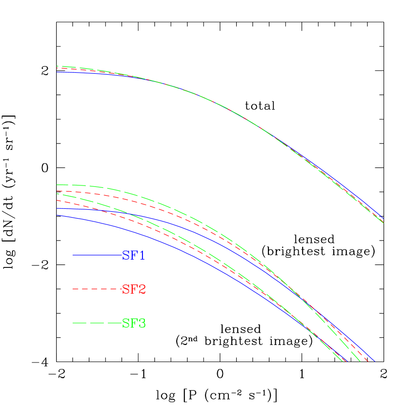
Figure 5.— Theoretical number counts of GRBs versus apparent peak photon flux (assuming a perfect detector with $\epsilon=1$ and full sky coverage). The solid, short–dashed and long–dashed lines refer to models in which the burst rate has been assumed to be proportional to the star formation histories SF1, SF2, and SF3, respectively. The upper set of curves shows the counts in absence of any lensing effect. From top to bottom, the remaining two sets depict the expected number counts for the brightest and the second brightest images of strongly lensed GRBs.

Figure 6.— The magnification bias $B$ (quantifying the fractional excess of lensed images in a flux–limited sample of GRBs relative to a volume limited sample) is plotted versus limiting peak photon flux. Solid lines: Brightest image of strongly lensed GRBs. Dashed lines: Second brightest image of multiply–imaged bursts.

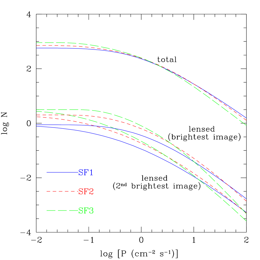
Figure 7.— Same as Figure 5, but for the total counts accumulated by the BAT onboard Swift during 3 years of observations. A field–of–view of 2 sr was assumed.

References

- (1)
- (2) Band, D. L., et al. 1993, ApJ, 413, 281
- (3)
- (4) Bardeen, J. M., Bond, J. R., Kaiser, N., & Szalay, A. S. 1986, ApJ, 304, 15
- (5)
- (6) Blain, A. W., Kneib, J–P., Ivison, R. J., & Smail, I. 1999, ApJ, 512, L87
- (7)
- (8) Blain, A. W., & Natarajan, P. 2000, MNRAS, 312, L39
- (9)
- (10) Bloom, J. S., et al. 1998, ApJ, 506, L105
- (11)
- (12) Bloom, J. S., Sigurdsson, S., & Pols, O. R. 1999, MNRAS, 305, 763
- (13)
- (14) Castro, S. M., et al. 2000, GCN Report 605
- (15)
- (16) Costa, E., et al. 1997, Nature, 387, 783
- (17)
- (18) Cowie, L. L., Songaila, A., & Barger, A. J. 1999, AJ, 118, 603
- (19)
- (20) Ellis, R. S., Colless, M., Broadhurst, T., Heyl, J., & Glazebrook, K. 1996, MNRAS, 280, 235
- (21)
- (22) Eke, V. R., Cole, S., & Frenk, C. S. 1996, MNRAS, 282, 263
- (23)
- (24) Fenimore, E. E., & Bloom, J. S. 1995, ApJ, 453, 25
- (25)
- (26) Fruchter, A. S., et al. 1999, ApJ, 520, 54
- (27)
- (28) Galama, T. J., et al. 1998, Nature, 395, 670
- (29)
- (30) Gould, A., Bahcall, J. N., & Flynn, C. 1996, ApJ, 465, 759
- (31)
- (32) Grossman, S. A. & Nowak, M. A. 1994, ApJ, 435, 548
- (33)
- (34) Hakkila, J., et al. 1998, in Gamma–ray Bursts: 4th Huntsville Symposium, ed. C. A. Meegan, R. D. Preece, & T. M. Koshut (New York: AIP), 144
- (35)
- (36) Holz, D. E., Miller, M. C., & Quashnock, J. M. 1999, ApJ, 510, 54
- (37)
- (38) Horack, J. M., Mallozzi, R. S., & Koshut, T. M. 1996, ApJ, 466, 21
- (39)
- (40) Keeton, C. R. 1998, PhD thesis, Harvard University
- (41)
- (42) Kochanek, C. S. 1993, ApJ, 419, 12
- (43)
- (44) Kommers, J. M., et al. 2000, ApJ, 533, 696
- (45)
- (46) Krumholz, M., Thorsett, S. E., & Harrison, F. A. 1998, ApJ, 506, L81
- (47)
- (48) Lamb, D. Q., & Reichart, D. E. 2000, ApJ, 536, 1
- (49)
- (50) Lloyd, N. M., & Petrosian, V. 1999, ApJ, 511, 550
- (51)
- (52) MacFadyen, A., & Woosley, S. E. 1999, ApJ, 524, 262
- (53)
- (54) Madau, P., della Valle, M., & Panagia, N. 1998, MNRAS, 297, 17
- (55)
- (56) Madau, P., Ferguson, H. C., Dickinson, M. E., Giavalisco, M., Steidel, C. C., & Fruchter, A. 1996, MNRAS, 283, 1388
- (57)
- (58) Madau, P., & Pozzetti, L. 2000, MNRAS, 312, L9
- (59)
- (60) Mao, S. 1992, ApJ, 389, L41
- (61)
- (62) Maoz, D., & Rix, H.–W. 1993, ApJ, 416, 425
- (63)
- (64) Marani, G. F. 1998, Ph.D. thesis, George Mason Univ.
- (65)
- (66) Marzke, R. O., da Costa, L. N., Pellegrini, P. S., Willmer, C. N. A., & Geller, M. J. 1998, ApJ, 503, 617
- (67)
- (68) Meegan, C. A., et al. 1992, Nature, 355, 143
- (69)
- (70) Navarro, J. F., Frenk, C. S., & White, S. D. M. 1997, ApJ, 490, 493
- (71)
- (72) Norris, J. P., 1996, in AIP Conf. Proc. 384, 3rd Huntsville Symp., Gamma–ray Bursts, ed. C. Kouveliotou, M. Briggs, & G. Fishman (New York: AIP), 77
- (73)
- (74) Norris, J. P., et al. 1994, ApJ, 424, 540
- (75)
- (76) Norris, J. P., et al. 1995, ApJ, 439, 542
- (77)
- (78) Nowak, M. A., & Grossman, S. A. 1994, ApJ, 435, 557
- (79)
- (80) Paciesas, W. S., et al. 1999, ApJS, 122, 465
- (81)
- (82) Paczyński, B. 1986, ApJ, 308, L43
- (83)
- (84) Paczyński, B. 1998, ApJ, 494, L45
- (85)
- (86) Pian, E., et al. 2000, ApJ, 536, 778
- (87)
- (88) Porciani, C., & Madau, P. 2000, ApJ, 532, 679
- (89)
- (90) Preece, R. D., et al. 2000, ApJS, 126, 19
- (91)
- (92) Press, W. H., & Schechter, P. 1974, ApJ, 187, 425
- (93)
- (94) Sahu, K., et al. 1997, ApJ, 489, L127
- (95)
- (96) Schmidt, M. 1999, ApJ, 523, L117
- (97)
- (98) Smith, D. A., Hurley, K., & Cline, T. 2000, GCN Report 568
- (99)
- (100) Steidel, C. C., Adelberger, K. L., Giavalisco, M., Dickinson, M., & Pettini, M. 1999, ApJ, 519, 1
- (101)
- (102) Stern, B. E., et al. 2000, ApJ, 540, L21
- (103)
- (104) Totani, T. 1997, ApJ, 486, L71
- (105)
- (106) Totani, T. 1999, ApJ, 511, 41
- (107)
- (108) Turner, E. L., Ostriker, J.P., & Gott, J. R., III 1984, ApJ, 284, 1
- (109)
- (110) van Paradijs, J., et al. 1997, Nature, 386, 686
- (111)
- (112) Wambsganns, J. 1993, ApJ, 406, 29
- (113)
- (114) Wijers, R. A. M. J., Bloom, J. S., Bagla, J. S., & Natarajan, P. 1998, MNRAS, 294, L13
- (115)