The MACHO Project Hubble Space Telescope Follow-Up: Preliminary Results on The Location of the Large Magellanic Cloud Microlensing Source Stars

Abstract

We attempt to determine whether the MACHO microlensing source stars are drawn from the average population of the LMC or from a population behind the LMC by examining the HST color-magnitude diagram (CMD) of microlensing source stars. We present WFPC2 HST photometry of eight MACHO microlensing source stars and the surrounding fields in the LMC. The microlensing source stars are identified by deriving accurate centroids in the ground-based MACHO images using difference image analysis (DIA) and then transforming the DIA coordinates to the HST frame. We consider in detail a model for the background population of source stars based on that presented by Zhao, Graff & Guhathakurta. In this model, the source stars have an additional reddening $<E(B-V)>=0.13$ mag and a slightly larger distance modulus $<\Delta\mu>\sim 0.3$ mag than the average LMC population. We also investigate a series of source star models, varying the relative fraction of source stars drawn from the average and background populations and the displacement of the background population from the LMC. Due to the small number of analyzed events the distribution of probabilities of different models is rather flat. A shallow maximum occurs at a fraction $s_{\rm LMC}\sim 0.8$ of the source stars in the LMC. This is consistent with the interpretation that a significant fraction of observed microlensing events are due to lenses in the Milky Way halo, but does not definitively exclude other models.

1 Introduction

The crucial observable in microlensing, the event duration, admits degeneracy in the three fundamental microlensing parameters: the mass, distance and velocity of the lens. This makes it difficult to distinguish between the two principal geometric arrangements which may explain Large Magellanic Cloud (LMC) microlensing: a) MW-lensing, in which the lensed object is part of the Milky Way (MW) and b) self-lensing, in which the lensed object is part of the LMC. In self-lensing, the lens may belong to the disk+bar, halo or “shroud” of the LMC, while the source star may come from any of these components or some sort of background population to the LMC.

Most efforts to distinguish between MW-lensing and self-lensing event distributions focus on modeling the LMC self-lensing contribution to the optical depth and comparing this to the observed optical depth. Early works by Sahu (1994) and Wu (1994) considered the traditional LMC self-lensing geometry in which both the source and lens are in the disk+bar of the LMC. Both works suggested that disk+bar self-lensing could account for a substantial fraction of the observed optical depth. This claim has since been disputed by several other groups (Gould, 1995; Alcock et al., 1997, 2000a) who show that when considering only disk stars the rate of LMC self-lensing is far too low to account for the observed rate. Gyuk, Dalal, & Griest (2000) show that allowing for contributions to the lens and source populations from the LMC bar does not substantially increase the LMC self-lensing optical depth. Alves & Nelson (2000) find a low LMC self-lensing optical depth for a flared LMC disk. Gyuk, Dalal, & Griest (2000) also show that much of the disagreement in models of the disk+bar self-lensing optical depth results from disagreement about the fundamental parameters of the LMC, such as the total disk mass and inclination angle. Within their region of allowed parameters Gyuk, Dalal, & Griest (2000) also make a strong case that disk+bar self-lensing makes a small contribution to the observed optical depth, at most $\sim$20%.

However, self-lensing becomes a much more plausible hypothesis if one allows for lenses in an LMC stellar halo population. The principal problem surrounding an LMC stellar halo contribution is that no tracers of old populations in the LMC have ever revealed a population with high enough velocity dispersions to suggest a virialized spheroidal component (Olszewski, Suntzeff & Mateo, 1996).

Recently however, a new possibility has arisen from the results of Weinberg (2000) who claims that LMC microlensing may be caused by a non-virialized stellar halo or “shroud”. This term was introduced by Evans & Kerins (2000) and is meant to imply an LMC population which is like a halo in that it is spacially not part of the LMC disk, but unlike a halo in that it is non-virialized and thus may have a relatively low velocity dispersion. Such a population is suggested by the simulations of Weinberg (2000) who finds that the LMC’s dynamical interaction with the MW may torque the LMC disk in such a way that the LMC disk is thickened and a spheroid component is populated without isotropizing the stellar orbits and thereby leaving disklike kinematics intact. Statistically marginal evidence for such a kinematically distinct population is found observationally in a study of carbon star velocities by Graff et al. (2000).

However, observational work on RR Lyrae by Kinman et al. (1991), which does not rely on the specific kinematics of the spheroidi, limits the total mass of any type of halo (virialized or non-virialized) to perhaps 5% of the mass of the LMC, too small to contribute more than $\sim$5% of the observed optical depth. A more recent revisiting of this argument by Alves (2000) finds room to increase this optical depth contribution to at most 20%, still only a small fraction of the total.

In order for an LMC shroud to account for the total optical depth it must have a mass comparable to that of the LMC disk+bar (Gyuk, Dalal, & Griest, 2000). Even if we accept the existence of such a massive shroud, the microlensing implications are somewhat in dispute. Weinberg (2000) finds an LMC self-lensing optical depth comparable to the observed optical depth. However, this estimate is reduced by a factor of three by Gyuk, Dalal, & Griest (2000) who repeat the Weinberg (2000) microlensing analysis using lower values for the disk total mass and inclination angle and a proper weighting over all observed MACHO fields.

Yet another self-lensing geometry was introduced by Zhao (1999) who suggests that the observed events are due to “background” self-lensing in which the source stars are located in some background population, displaced at some distance behind the LMC. A veritable plethora of lenses for this population is then supplied by the disk+bar of the LMC. A background population has the advantage of being nearly impossible to confirm or reject observationally, as there are nearly no limits on its size or content (provided of course, it is small enough to “hide” behind the LMC).

A final possibility is “foreground” self-lensing. This is not self-lensing in the classical sense as in this case the lenses are not drawn from the LMC itself, but rather from some kinematically distinct foreground population, such as an intervening dwarf galaxy. Zaritsky & Lin (1997) claim a detection of a population of stars from such an entity. However, Beaulieu & Sackett (1998) claim that this “population” is a morphological feature of the LMC red clump, while others show that such a population consistent with other observational constraints could not produce a substantial microlensing signal (Gould, 1998; Bennett, 1998).

In this work we attempt to determine whether the MACHO source stars belong to the average population of the LMC or to a background population displaced at some distance behind the LMC disk. The determination of source star location is based on the suggestion of Zhao (1999), Zhao (2000), and Zhao, Graff & Guhathakurta (2000) who point out that source stars from a background population should be preferentially fainter and redder than the average population of the LMC due to the extinction of the LMC disk and their displacement along the line of sight. Zhao, Graff & Guhathakurta (2000) present a model for this background population with an additional mean reddening relative to the average population of the LMC $<E(B-V)>=0.13$ mag and a displacement from the LMC of $\sim 7.5$ kpc resulting in an increase of distance modulus of $<\Delta\mu>\sim 0.3$ mag.

The location of the source stars has implications for the location of the lenses and thus for the nature of LMC microlensing. If all the source stars are in the background population, then the great majority of the lenses are found in the LMC disk+bar and LMC microlensing is dominated by background self-lensing. Conversely, if all the source stars are in the LMC, then microlensing may be due to MW-lensing, disk+bar self-lensing or foreground self-lensing. However, since the contribution from disk+bar self-lensing has been shown to be small and the evidence for a foreground intervening population is unconvincing, a result which places all source stars in the LMC would suggest that LMC microlensing is dominated by MW-lensing. If, however, we find a more equal division of source stars between the LMC and the background population then this implies either some mixture of MW-lensing and disk+bar self-lensing, or a more symmetric self-lensing geometry such as the LMC shroud discussed above.

We first investigate two models: the first putting all source stars in the LMC (Model 1), and the second putting all source stars in a background population (Model 2). We compare a Hubble Space Telescope (HST) CMD of MACHO microlensing source stars to efficiency weighted CMDs of the average population of the LMC and the Zhao, Graff & Guhathakurta (2000) background population. In §2 we construct a CMD of the average LMC population by combining the CMDs of eight HST Wide Field Planetary Camera 2 (WFPC2) fields centered on past MACHO microlensing events in the outer LMC bar. In §3 we describe the identification of the microlensing source stars in these fields by difference image analysis (DIA). In §4 we construct the background population CMD by shifting the HST CMD by the appropriate amount of extinction and distance modulus. We then describe the convolution of the average and background HST CMDs with the MACHO efficiency for detecting a microlensing event in a source star of given magnitude. In §5 we determine the likelihoods that the microlensing source stars were drawn from the average population of the LMC (Model 1) and from a population of background source stars (Model 2) by using Kolmogorov-Smirnov (KS) tests to compare our observed and model distributions. Finally, in §6 we generalize our analysis and consider intermediate models with varying distance moduli and fractions of source stars in the background and LMC. We conclude and discuss the implications for the location of the lenses in §7.

2 HST Observations

Observations were made with the WFPC2 on HST between May 1997 and October 1999 through the F555W ($V$) and F814W ($I$) filters. The Planetary Camera (PC) was centered on the location of past MACHO microlensing events. The microlensing events, positions, and exposure times are listed in Table 1.

Multiple exposures of a field were combined using a sigma-clipping algorithm to remove deviant pixels, usually cosmic rays. The PC has a pixel size of $0.046^{\prime\prime}$ which easily resolves the great majority of stars in our frames. Most stars are also resolved in the Wide Field (WF) fields which have a pixel size of $0.1^{\prime\prime}$. Instrumental magnitudes were calculated from aperture photometry using DAOPHOT II (Stetson, 1987, 1991) with a radius of $0.25^{\prime\prime}$ and centroids derived from point-spread function (PSF) fitting photometry. Aperture corrections to $0.5^{\prime\prime}$ were performed individually for each frame. We correct for the WFPC2 charge transfer effect using the equations from Instrument Science Report WFPC2 97-08. We also make the minimal corrections for contaminants which adhere to the cold CCD window according to the WFPC2 Instrument Handbook. We transform our instrumental magnitudes to Landolt $V$ and $I$ using the calibrations from Holtzman et al. (1995).

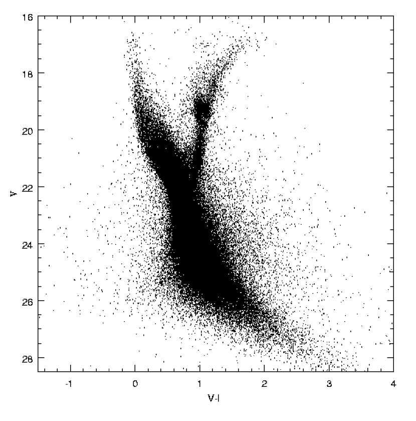
Figure 1: The composite HST CMD created by combining the photometry from 8 WFPC2 fields centered on observed MACHO microlensing events.

We create a composite LMC CMD by combining the PC and WF photometry for all of our fields except the field of LMC-1. In the case of LMC-1 the $V$ and $I$ observations were taken at different roll angles and there is little area of overlap except in the PC frame. We therefore include the PC field from LMC-1 but not the WF fields. The composite HST CMD is shown in Figure 1.

3 Source Star Identification through Difference Image Analysis

A ground-based MACHO image has a pixel size of $0.6^{\prime\prime}$ and a seeing of at least $1.5^{\prime\prime}$. Thus, in a typically crowded region of the outer LMC bar, a MACHO seeing disk will contain $\sim$11 stars of $V\lesssim 24$. This means that faint “stars” in ground-based MACHO photometry are usually not single stars at all, but rather blended composite objects made up of several fainter stars. Henceforth, we distinguish between these two words carefully, using object to denote a collection of stars blended into one seeing disk, and star to denote a single star, resolved in an HST image or through DIA. The characteristics of the MACHO object that was lensed tell us little about the actual lensed star. However, with the microlensing object centroid from the MACHO images we can hope to identify the microlensing source star in the corresponding HST frame.

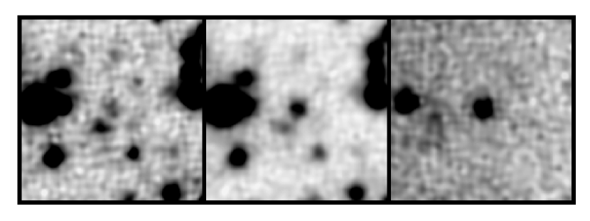
Figure 2: The left panel shows a 0.6’ X 0.6’ section of the baseline image of MACHO event LMC-4. The middle panel shows the same region taken at the peak of the microlensing event. The right panel shows the differenced image. The flux at the left hand side of the differenced image is due to an asymptotic giant branch variable star at that location.

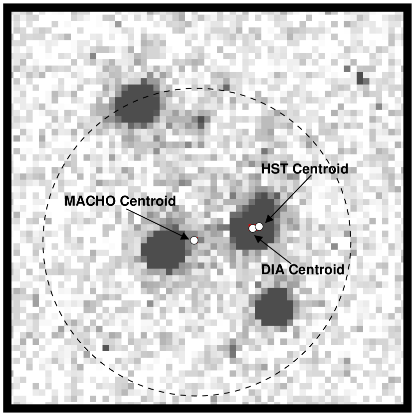
Figure 3: A 3” X 3 ” HST image of LMC-4. The circle contains the several HST stars which are all contained within the MACHO seeing disk of the lensed object. The arrows indicate the MACHO baseline centroid, the DIA centroid and the HST centroid.

A direct coordinate transformation from the MACHO frame to the HST frame often places the baseline MACHO object centroid in the middle of a cluster of faint HST stars with no single star clearly identified. To resolve this ambiguity we have used DIA. This technique is described in detail in Tomaney & Crotts (1996), but we review the main points here. DIA is an image subtraction technique designed to provide accurate photometry and centroids of variable stars in crowded fields. The basic idea is to subtract from each program image a high signal-to-noise reference image, leaving a differenced image containing only the variable components. Applied to microlensing, we subtract baseline images from images taken at the peak of the microlensing light curve, leaving a differenced image containing only the flux from the microlensing source star and not the rest of the object. We also find a centroid shift between the baseline image and the differenced image towards the single star that was microlensed. If the centroid from the differenced image is transformed to the HST frame we find that it usually clearly identifies the HST microlensed source star. This process is illustrated in Figures 2 and 3.

This technique allows us to unambiguously identify 7 of 8 microlensed source stars. In the case of LMC-9 the DIA centroid lands perfectly between two stars; fortunately these two stars are virtually identical sub-giants and the choice between the two has no effect on our results. In Table 2 we present the $V$ magnitudes and $(V-I)$ colors of our source stars from the HST data. The errors presented here are the formal photon counting errors returned by DAOPHOT II. We estimate that all WFPC2 magnitudes have an additional $0.02-0.03$ mag uncertainty due to aperture corrections. In the case of LMC-9 we tabulate both possibilities and use LMC-9a in the remainder of this work.

Our identification of LMC-5 revealed it to be the rather rare case of a somewhat blended HST star. Although there are two stars evident, at an aperture of $0.25^{\prime\prime}$ the flux of one star was contaminated by that of its neighbor. Therefore, in this case, we perform PSF fitting photometry using PSFs kindly provided by Peter Stetson. The errors presented in Table 2 for LMC-5 are those returned by the profile fitting routine ALLSTAR. The DIA centroid falls 2 pixels closer to the centroid of star one than star two, clearly preferring star one as the source star. Furthermore, as predicted by Alcock et al. (1997) and Gould, Bahcall, & Flynn (1997), star two is a rather red object which is very faint in the V band. Fits to the MACHO lightcurve presented in Alcock et al. (2000a) suggest lensed flux fractions in the V and R bands of 1.00 and 0.46 respectively, confirming the DIA choice of the much bluer star as the lensed source star.

Since this work specifically addresses the background lensing geometry, we also discuss here the (remote) possibility that our HST images of the source stars are actually completely blended objects consisting of a faint background source star and a brighter LMC lens. Such a configuration would seriously skew our CMD distribution of source stars as we would instead be presenting photometry of the lenses. We begin by noting that the MACHO efficiency for detection of a microlensing event in a star has fallen to zero at $V\sim 22.5$ (see Figure 4 and explanation below). This means that a “faint” background source star must have $V_{S}<22.5$ in order to produce a detectable event. The the lens in this scenario is assumed to have $V_{L}<V_{S}$. We estimate that we would not recognize a blended object of two stars with $V<22.5$ as such if the centroids coincided to within 1.5 pixels. In our most crowded PC field we find $\sim$1000 stars with $V<22.5$ spread over an area of 720 X 720 pixels. In simulations, we draw 1000 stars with $V<22.5$ weighted according to our luminosity function and spread randomly over 720X720 pixels. For each star we then check to see if it is found within 1.5 pixel of a brighter star. We find that on average, there will be 5 stars of $V<22.5$ which are blended with a brighter star. Therefore, for our most crowded field, the chance that our source star is an unrecognized blend of a faint source star and a brighter lens is about 5 in a thousand. In a more typically crowded field, this falls to around 1 chance in 1000. Therefore, it is extremely unlikely that any of our 8 HST source stars are blended objects composed of a faint source star and a bright lens.

4 Creation of the model source star populations

If the microlensing events are due to MW lenses, then one would expect the distribution of observed microlensing source stars to be randomly drawn from the average population of the LMC corrected only for the MACHO detection efficiency for stars of a given magnitude (Model 1). We assume that the population of the LMC is well represented by our composite HST CMD to $V\lesssim 24$. If the microlensing events are background self-lensing events we expect the source stars to be drawn from a background population which suffers from the internal extinction of the LMC (Model 2). To represent such a background population we shift the composite HST CMD according to the amounts suggested by Zhao, Graff & Guhathakurta (2000), $<E(B-V)>=0.13$ and $\Delta\mu=0.3$. Since, Holtzman et al. (1995) calibrate instrumental WFPC2 magnitudes to the Landolt system, we use the appropriate Landolt system extinction coefficients of Table 6 in Schlegel, Finkbeiner & Davis (1998) to translate these estimates to our filters. The total shifts, taking into account both reddening and distance modulus, are

$$\Delta V=A_{V}+\Delta{\mu}=0.73,~{}~{}\Delta(V-I)=E(V-I)=0.18~{}~{}~{}~{}~{}~{}~{}(Model~{}2)$$

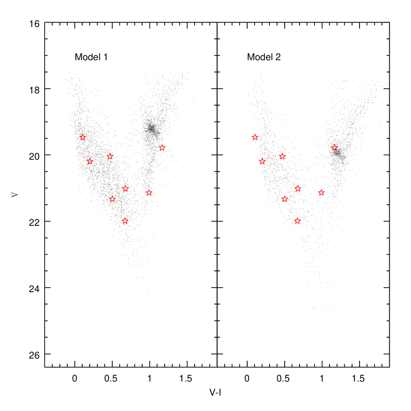
Figure 5: The model source star populations. Model 1 represents a source star population in the disk of the LMC, Model 2 represents a source star population behind the LMC. The MACHO microlensing events of Table 2 are overplotted in red. We perform 2-D KS tests to determine the probability that the microlensing events are drawn from each model source star populations. We find probabilities $P_{1}=0.319\pm 0.027$ and $P_{2}=0.103\pm 0.023$ that the microlensing events are consistent with the source star populations of Models 1 and 2, respectively.

Thus far we have constructed two CMDs representing the distribution of all possible source stars down to $V\sim 24$. However, not all possible microlensing events are detected in the MACHO images. To create a CMD representing a population of source stars which produce detectable microlensing events we must convolve the HST CMD with the MACHO detection efficiency. The MACHO efficiency pipeline is extensively described in Alcock et al. (2000a) and Alcock et al. (2000b) and the detection efficiency as a function of stellar magnitude, $V_{\rm{star}}$, and Einstein ring crossing time has been calculated. We average this function over the event durations of the candidate microlensing events derived using detection criterion A from Alcock et al. (2000a) and present the MACHO detection efficiency as a function of $V_{\rm{star}}$ in Figure 4. We convolve this function with our HST CMDs to produce the final Model 1 and 2 distributions of source stars. In Figure 5, we show our model source star populations with the observed microlensing source stars of Table 2 overplotted as large red stars.

This procedure admits several assumptions. First, we assume that our eight HST fields collectively well represent the stellar population of the LMC disk. This assumption has two parts, the first being that an observation at a random line of sight in the LMC bar is dominated by stars in the LMC disk and the second that the stellar population across the LMC is fairly constant. The first part holds so long as the surface density of the background population is much smaller than that of the LMC itself. If this were not the case, this population would have been directly detected. The second part has been confirmed by many LMC population studies including Alcock et al. (2000b), Olsen (1999), and Geha et al. (1998), as well as our own comparison of individual CMDs and luminosity functions. Second, we assume that the underlying stellar content of the background population is identical to that of the LMC.

5 The Location of the Source Stars

We now attempt to determine whether the CMD of microlensed source stars is consistent with the average population of the LMC (Model 1) or whether it is more consistent with a background population (Model 2) by performing a two-dimensional Kolmogorov-Smirnov (KS) test.

In the familiar one dimensional case, a KS test of two samples with number of points $N_{1}$ and $N_{2}$ returns a distance statistic $D$, defined to be the maximum distance between the cumulative probability functions at any ordinate. Associated with $D$ is a corresponding probability $P(D)$ that if two random samples of size $N_{1}$ and $N_{2}$ are drawn from the same distribution a worse value of $D$ will result. This is equivalent to saying that we can exclude the hypothesis that the two samples are drawn from the same distribution at a confidence level of $1.0-P(D)$. If $N_{2}\gg N_{1}$ then this is also equivalent to excluding at a $1.0-P(D)$ confidence level the hypothesis that sample 1 is drawn from sample 2.

The concept of a cumulative distribution is not defined in more than one dimension. However, it has been shown that a good substitute in two dimensions is the integrated probability in each of four right-angled quadrants surrounding a given point (Fasano & Franceschini, 1987; Peacock, 1983). Leaving aside the exact algolrithmic definition (Press et al., 1992) a two-dimensional KS test yields a distance statistic $D$ and a corresponding $P(D)$ with the same interpretation as in the one dimensional case.

We use the two-dimensional KS test to test hypothesis that the CMD of observed MACHO microlensing events is drawn from the same population as each of the model source star distributions. We find distance statistics $D_{1}=0.394\pm 0.005$ and $D_{2}=0.473\pm 0.009$, for Models 1 and 2 respectively. Each of these distance statistics has a corresponding probability, $P(D)$, that if we draw an 8 star samples from the model population a larger value than $D$ will result. As explained above, this is equivalent to excluding this model population as the actual parent of our observed microlensing source stars at a confidence level of $1.0-P(D)$. These probabilities are $P_{1}=0.319\pm 0.027$ and $P_{2}=0.103\pm 0.023$. The error quoted for each of these quantities is the scatter about the mean value in 50 simulations for each model. Because the creation of the efficiency convolved CMD is a weighted random draw from the HST CMD, the model population created in each simulation differs slightly. This in turn leads to small differences in the KS statistics.

These results tell us that these 8 MACHO events are insufficient to reliably distinguish the MW and self lensing hypothesis. The best we can do is to exclude Model 2 at the statistically marginal 90% confidence level.

6 Intermediate Models

Thus far we have considered the possibilities that the observed MACHO source stars are either all LMC stars or all background stars at a mean distance of $\sim 7.5$ kpc behind the LMC. However, as discussed in Zhao (1999), Zhao (2000) and Zhao, Graff & Guhathakurta (2000) there is substantial middle ground. In a complete analysis, we may treat both the fraction of source stars drawn from the background population and the distance to the background population as adjustable parameters. While the size, location and content of the LMC has been well constrained by observations, the existence, size and location of a background population is constrained only by the fact that it must be small enough to have evaded direct detection. The distance to the background population from Zhao, Graff & Guhathakurta (2000) is very loosely derived by the requirement that the background population be at least transiently gravitationally bound to the LMC. However, the reddening of a background population is a much more physically constrained number since a population behind the LMC should certainly suffer from the mean internal extinction of the LMC, a number which has been well determined in a number of studies including Oestricher & Schmidt-Kaler (1996) and Harris, Zaritsky & Thompson (1997). Therefore, all our background population models have the same reddening $<E(B-V)>=0.13$, as inferred from the mean extinction of the LMC from Harris, Zaritsky & Thompson (1997) corrected for Galactic foreground extinction.

We define $s_{\rm LMC}$ to be the fraction of the source stars drawn from the LMC disk+bar population, leaving a fraction $1.0-s_{\rm LMC}$ source stars drawn from the background population, and $\Delta\mu$ to be the excess distance modulus of the background population. We consider values $\Delta\mu=0.0,0.30,0.45$ and for each value of the distance modulus we consider the full range of $s_{\rm LMC}$ from 0.0 to 1.0. For example, a model with $\Delta\mu=0.45$ and $s_{\rm LMC}=0.5$ contains a mixture of source stars in which half the source stars are drawn from the population of the LMC disk, and half the source stars are drawn from a background population displaced from the LMC by $\sim 11$kpc and reddened by $<E(B-V)>=0.13$. All models with $s_{\rm LMC}=0.0$ contain only source stars drawn from a specified background population, and all models with $s_{\rm LMC}=1.0$ are identical, containing only stars drawn from the LMC disk.

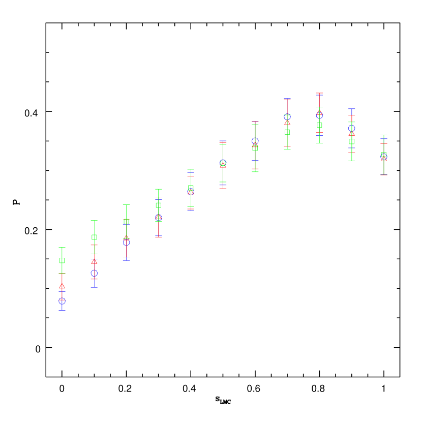
Figure 6: The KS test probabilities, P, for various values of the fraction of source stars in the LMC, $s_{\rm LMC}$, and the displacement of the background population, $\Delta\mu$. We show the results for $\Delta\mu=0.45,0.30,0.0$ in blue circles, red triangles and green squares, respectively. The error bars indicate the scatter around the mean value of 50 simulations done for each model.

We present the results in Figure 6, showing the KS test probabilities as a function of $s_{\rm LMC}$ for each of our values of $\Delta\mu$. Again, the error bars reflect the scatter about the mean for fifty simultations of each model. We note that since all models with $s_{\rm LMC}=1.0$ contain only source stars drawn from the LMC disk, all curves for different $\Delta\mu$ must converge at $s_{\rm LMC}=1.0$. Furthermore, we learn from Figure 6 that the value of $\Delta\mu$ makes little difference even at $s_{\rm LMC}=0.0$. So long as the background population is behind the LMC and therefore reddened by $<E(B-V)>=0.13$ its exact displacement is of little import. In all cases a smaller value of $\Delta\mu$ flattens the curves somewhat. This is expected as a smaller value of $\Delta\mu$ implies overall less difference between the two extreme models at $s_{\rm LMC}=0.0$ and $s_{\rm LMC}=1.0$. The two dimensional KS test of the CMD displays a shallow maximum at $s_{\rm LMC}\sim 0.8$.

7 Discussion

We have compared two models for LMC microlensing: source stars drawn from the average population of the LMC and source stars drawn from a population behind the LMC. By comparing the CMD of observed microlensing source stars to a CMD representing all detectable microlensing events for each of these models we find by two-dimensional KS tests that the data suggest that it is more likely that all the source stars are in the LMC than that all the source stars are in the background. However, we can only exlude the possibility that all the source stars are in the background at a statistically marginal 90% confidence level.

We also consider a number of intermediate models in which we vary the distance modulus of the background population as well as the fraction of stars drawn from average and background populations. In these models we find that for all displacements the most highest probability occurs for a fraction $s_{\rm LMC}\sim 0.8$ LMC source stars and $s_{\rm BKG}=1.0-s_{\rm LMC}=0.2$ background source stars. We also find that the value of the distance modulus has very little effect on our results at all values of $s_{\rm LMC}$.

Our results are completely consistent with the interpretation that MACHO microlensing events are dominated by MW-lensing. In the MW-lensing geometry, the source stars reside in the LMC and the lenses are in the halo or disk of the MW. The MW-lensing interpretation for microlensing requires that $s_{\rm LMC}\sim 1.0$, consistent with our result. We note that both disk+bar self-lensing and foreground self-lensing also place all their source stars in the LMC. However, these contributions to the number of events have been shown to be small and we neglect their contribution here. We also note that the contribution from the known stellar populations of the MW is expected to be small ($\sim$1 events of the 13-event cut A sample of Alcock et al. (2000a) but not entirely negligible. A lens population in the MW is likely to be dominated by MACHOs in the MW halo and not faint stars in the MW disk or spheroid.

Zhao (1999), Zhao (2000) and Zhao, Graff & Guhathakurta (2000) propose a model for LMC microlensing in which all the source stars are drawn from some background population to the LMC. Such a model suggests that LMC microlensing is dominated by background self-lensing and that $s_{\rm LMC}\sim 0.0$. We find this arrangement to be the model excluded at the highest confidence; however, we cannot rule it out with any great statistical weight.

Recently, Weinberg (2000) and Evans & Kerins (2000) have suggested a model of LMC microlensing in which all microlensing events are due to a non-virialized shroud of stars which surrounds the LMC. In shroud self-lensing there are four event geometries: a) background shroud source and disk lens, b) disk source and foreground shroud lens, c) disk source and disk lens and d) background shroud source and foreground shroud lens. We might naively expect the former two types dominate the number of expected events and so if we were to ignore the contribution from the latter two types we would conclude that shroud lensing would imply $s_{\rm LMC}\sim 0.5$. However, in order to produce the entire observed optical depth, the shroud must be so massive that it is no longer self-consistent to ignore the latter terms. Calculations performed in the formalism of Gyuk, Dalal, & Griest (2000) suggest instead that events with a background shroud source and a foreground shroud lens become an important contributor and reduce the expected fraction of source stars in the LMC to $s_{\rm LMC}\sim 0.3-0.4$. Our results are not inconsistent with such a model, however we note that there is a profound lack of observational evidence for such a stellar shroud.

Furthermore, if we assume that a substantial LMC stellar halo or shroud is not a realistic possibility, then we may directly relate the fraction of source stars in the LMC, $s_{\rm LMC}$, to the fraction of microlensing events which are MW-lensing, $f_{\rm MW}$ in the following way. All events in which the source stars are located in the background are, by definition, background lensing events. Therefore, $s_{\rm BKG}=f_{\rm BKG}$, where $f_{\rm BKG}$ indicates the fraction of observed events which are background lensing. The total fraction of lensing events due to halo-lensing $f_{\rm MW}$, LMC self-lensing, $f_{\rm LMC}$, and background self-lensing, $f_{\rm BKG}$, must be equal to unity.

$$f_{\rm MW}+f_{\rm LMC}+f_{\rm BKG}=1.0$$ (1)

This may be rearranged to read

$$f_{\rm MW}=1.0-f_{\rm BKG}-f_{\rm LMC}=s_{\rm LMC}-f_{\rm LMC}$$ (2)

Equation (2) is strictly true even if we allow for LMC shroud lensing. However, if we ignore the possibility of LMC self-lensing by a non-virialized stellar shroud, then all models with reasonable parameters for the LMC find that $f_{\rm LMC}\lesssim 0.2$. Therefore, if $s_{\rm LMC}\sim 1$, we may make the approximation

$$f_{\rm MW}\sim s_{\rm LMC}$$ (3)

Therefore we estimate, with low statistical significance due to the small sample size of our sample, that a fraction $f_{\rm MW}\sim 0.8$ of observed microlensing events are halo-lensing. We emphasize once again that this conclusion ignores the possibility of a non-virialized LMC shroud.

At present, the strength of this analysis is severely limited by the number of microlensing events for which we have corresponding HST data. A fortuitous distribution in the CMD of all 13 criterion A events presented in Alcock et al. (2000a) may allow us to definitively exclude a model in which all the source stars are drawn from the background population. It is difficult to estimate how many events are needed to definitely determine $s_{\rm LMC}$ as the number depends on the true value of $s_{\rm LMC}$ as well the degree of accuracy one wishes to achieve. However, when we perform Monte Carlo simulations where we draw a sample of N events from the distribution with $s_{\rm LMC}=0.0$ and compare it with the 2-D KS test to the distribution with $s_{\rm LMC}=1.0$ we find that for $N\sim 20-25$, $P<0.01$ for at least 99% of our simulations. This implies that if the true value of $s_{\rm LMC}$ is near either extreme ($s_{\rm LMC}\sim 0$ or $s_{\rm LMC}\sim 1$) then a CMD of 20-25 events virtually guarantees that we will be able to exclude a model at the other extreme at the 99% confidence level. Even more events are necessary to exclude intermediate models with various fractions of LMC and background stars. Ongoing microlensing search projects (EROS, OGLE II) may supply a sufficient sample of events in the next few years. The technique outlined in this paper should prove a powerful method for locating the lenses with these future datasets.

[f1.ps]

[f2.ps]

[f3.ps]

Figure 4: The MACHO detection efficiency as a function of stellar V-magnitude. That is, if a microlensing event occurs in a star of given magnitude $V_{star}$, this is the given efficiency for detecting that event.

[f4.ps]

[f5.ps]

[f6.ps]

Table 1: Summary of Observations

Event	RA	DEC	V Exposure Times	I Exposure Times	Obs Date
LMC-1	05:14:44.50	-68:48:00.00	4X400s	40X500s	1997-12-16
LMC-4	05:17:14.60	-70:46:59.00	4X400s	2X500s	1998-08-19
LMC-5	05:16:41.10	-70:29:18.00	4X400s	2X500s	1999-05-13
LMC-6	05:26:14.00	-70:21:15.00	4X400s	2X500s	1999-08-26
LMC-7	05:04:03.40	-69:33:19.00	4X400s	2X500s	1999-04-12
LMC-8	05:25:09.40	-69:47:54.00	4X400s	2X500s	1999-03-12
LMC-9	05:20:20.30	-69:15:12.00	4X400s	2X500s	1999-04-13
LMC-14	05:34:44.40	-70:25:07.00	4X500s	4X500s	1997-05-13

Table 2: Photometry of Microlensing Source Stars

Event	$V$	$V-I$
LMC-1	$19.782\pm 0.003$	$1.167\pm 0.004$
LMC-4	$21.331\pm 0.008$	$0.502\pm 0.009$
LMC-5	$21.016\pm 0.096$	$0.677\pm 0.122$
LMC-6	$20.041\pm 0.004$	$0.471\pm 0.007$
LMC-7	$21.993\pm 0.013$	$0.672\pm 0.022$
LMC-8	$20.195\pm 0.004$	$0.203\pm 0.009$
LMC-9a	$21.137\pm 0.007$	$0.991\pm 0.011$
LMC-9b	$21.250\pm 0.008$	$1.002\pm 0.012$
LMC-14	$19.467\pm 0.002$	$0.106\pm 0.004$

References

- Alcock et al. (1997) Alcock, C., et al. 1997, ApJ, 486, 697
- Alcock et al. (2000a) Alcock, C., et al. 2000a, ApJ, 542, 281
- Alcock et al. (2000b) Alcock, C., et al. 2000b, ApJ, in press, astro-ph/0003236
- Alves (2000) Alves, D.R. 2000, in “Galaxy Disks and Disk Galaxies,” eds. S.Funes & E. Corsini, astro-ph/0010098
- Alves & Nelson (2000) Alves, D.R. & Nelson, C.A. 2000, ApJ, 542, 789
- Beaulieu & Sackett (1998) Beaulieu, J., & Sackett, P. 1998, AJ, 116, 209
- Bennett (1998) Bennett, D.P. 1998, ApJ, 493, L79
- Evans & Kerins (2000) Evans, N.W. & Kerins, E. 2000, ApJ, 529, 917
- Fasano & Franceschini (1987) Fasano, G., & Franceschini, A. 1987, MNRAS, 225, 155
- Geha et al. (1998) Geha, M., et al. 1998, AJ, 115, 1045
- Gould (1995) Gould, A. 1995, ApJ, 441, 77
- Gould (1998) Gould, A. 1998, ApJ, 499, 728
- Gould, Bahcall, & Flynn (1997) Gould, A., Bahcall, J.N., & Flynn, C. 1997, ApJ, 482, 913
- Graff et al. (2000) Graff, D.S., Gould, A.P., Suntzeff, N.B., Schommer, R.A., & Hardy, E. 2000, ApJ, 540, 211
- Gyuk, Dalal, & Griest (2000) Gyuk, G., Dalal, N., & Griest, K. 2000, ApJ, 535, 90
- Harris, Zaritsky & Thompson (1997) Harris, J., Zaritsky, D., & Thompson, I. 1997, AJ, 114, 1933
- Holtzman et al. (1995) Holtzman, J.A., Burrows, C.J., Casertano, S., Hester, J.J., Trauger, J.T., Watson, A.M., & Worthey, G. 1995, PASP, 107, 1065
- Oestricher & Schmidt-Kaler (1996) Oestricher, M.O., & Schmidt-Kaler, T. 1996, A&AS, 117, 303
- Kinman et al. (1991) Kinman, T.D., et al. 1991, PASP, 103, 1279
- Olsen (1999) Olsen, K.A.G., 1999, AJ, 117, 2244
- Olszewski, Suntzeff & Mateo (1996) Olszewski, E.W., Suntzeff, N.B., & Mateo, M. 1996, ARA&A, 332, 1
- Peacock (1983) Peacock, J.A. 1983, MNRAS, 202, 615
- Press et al. (1992) Press, W.H., Teukolsky, S.A., Vetterling, W.T., & Flannery, B.P. 1992, Numerical Recipes in C, Second Edition (Cambridge: Cambridge Univ. Press)
- Sahu (1994) Sahu, K.S. 1994, Nature, 370, 275
- Schlegel, Finkbeiner & Davis (1998) Schlegel, D.J., Finkbeiner, D.P., & Davis, M. 1998, ApJ, 500, 525
- Stetson (1987) Stetson, P.B. 1987, PASP, 99, 191
- Stetson (1991) Stetson, P.B. 1991, Data Analysis Workshop III (Garching: ESO), 187
- Tomaney & Crotts (1996) Tomaney, A.B., & Crotts, A.P.S. 1996, AJ, 112, 2872
- Weinberg (2000) Weinberg, M. 2000, ApJ, 532, 922
- Wu (1994) Wu, X. 1994, ApJ, 435, 66
- Zaritsky & Lin (1997) Zaritsky, D., & Lin, D.N.C. 1997, AJ, 114, 2546
- Zhao (1999) Zhao, H. 1999, ApJ, 527, 167
- Zhao (2000) Zhao, H. 2000, ApJ, 530, 299
- Zhao, Graff & Guhathakurta (2000) Zhao, H., Graff, D.S., & Guhathakurta, P. 2000, ApJ, 532, L37
[f1.ps]
[f2.ps]
[f3.ps]
[f4.ps]
[f5.ps]
[f6.ps]