Cosmological-Model-Parameter Determination from Satellite-Acquired
Supernova Apparent Magnitude versus Redshift Data

Abstract

We examine the constraints that satellite-acquired supernova apparent magnitude versus redshift data will place on cosmological model parameters in models with and without a constant or time-variable cosmological constant $\Lambda$. Data which could be acquired in the near future will result in tight constraints on these parameters. For example, if all other parameters of a spatially-flat model with a constant $\Lambda$ are known, the supernova data should constrain the non-relativistic matter density parameter $\Omega_{0}$ to better than 1% (2%, 0.5%) at 1$\sigma$ with neutral (worst case, best case) assumptions about data quality.

1 Introduction

Recent applications of the apparent magnitude versus redshift test based on Type Ia supernovae (SNe Ia) have resulted in interesting constraints on cosmological-model parameters (see, e.g., Riess et al. 1998; Perlmutter et al. 1999; Podariu & Ratra 2000; Waga & Frieman 2000; Gott et al. 2001). Higher quality data will result in tighter constraints on cosmological-model parameters. A dedicated supernova space telescope could provide the high quality data needed to realize the full potential of this neoclassical cosmological test.

In this paper we examine constraints on cosmological-model parameters that will result from such a data set. For definiteness we focus on data that could be acquired by the proposed SNAP space telescope (Curtis et al. 2000 and http://snap.lbl.gov). That is, we assume a data set of 2000 SNe Ia multi-frequency light curves, for SNe out to redshift $z=2$, with errors discussed below.

Observational data favor models with a low $\Omega_{0}$. The simplest such models have either flat spatial hypersurfaces and a constant or time-variable cosmological “constant” $\Lambda$ (see, e.g., Peebles 1984; Peebles & Ratra 1988; Sahni & Starobinsky 2000; Steinhardt 1999; Carroll 2000; Binétruy 2000), or open spatial hypersurfaces and no $\Lambda$ (see, e.g., Gott 1982, 1997; Ratra & Peebles 1994, 1995; Kamionkowski et al. 1994; Górski et al. 1998). For a constant $\Lambda$ (with density parameter $\Omega_{\Lambda}$), these models lie along the lines $\Omega_{0}+\Omega_{\Lambda}=1$ and $\Omega_{\Lambda}=0$, respectively, in the more general two-dimensional ($\Omega_{0}$, $\Omega_{\Lambda}$) model-parameter space. Depending on the values of $\Omega_{0}$ and $\Omega_{\Lambda}$, models in this two-dimensional parameter space have either closed, flat, or open spatial hypersurfaces. In this paper we derive constraints on the parameters of the two-dimensional model as well as those of the special one-dimensional cases.

We also derive constraints on the parameters of a spatially-flat model with a time-variable $\Lambda$. The only known consistent model for a time-variable $\Lambda$ is that based on a scalar field ($\phi$) with a scalar field potential $V(\phi)$ (Ratra & Peebles 1988). In this paper we focus on the favored model which at low $z$ has $V(\phi)\propto\phi^{-\alpha}$, $\alpha>0$ (Peebles & Ratra 1988; Ratra & Peebles 1988). This model is in reasonable accord with observational data (see, e.g., Peebles & Ratra 1988; Ratra & Quillen 1992; Podariu & Ratra 2000; Waga & Frieman 2000; Brax, Martin, & Riazuelo 2000).

A scalar field is mathematically equivalent to a fluid with a time-dependent speed of sound (Ratra 1991), and it may be shown that with $V(\phi)\propto\phi^{-\alpha}$, $\alpha>0$, the $\phi$ energy density behaves like a cosmological constant that decreases with time. We emphasize that in our analysis of this model here we do not make use of the time-independent equation of state fluid approximation to the model that has sometimes been used for such computations (see the discussion in Podariu & Ratra 2000).

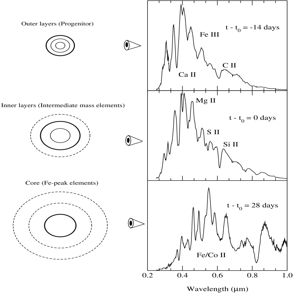
Figure 2: As the SN Ia evolves in time the rapid expansion of it’s atmosphere allows the observer to probe to deeper layers as the optical depth falls off with the diminishing density. At early times one views the outermost layers, mostly composed of the unburnt progenitor. Near peak brightness the intermediate mass elements of S II and Si II are quite visible. At later times, shortly after entering the nebular phase, one views the Fe-peak core of the SN Ia where the radioactive decay of $\approx$0.5 M_⊙ of ⁵⁶Ni has taken place since the explosion.

Huterer & Turner (1999), Starobinsky (1998), Nakamura & Chiba (1999), Saini et al. (2000), and Chiba & Nakamura (2000) discuss using supernova apparent magnitude versus redshift data to determine the scalar field potential of the time-variable $\Lambda$ model. This is a difficult task. Maor, Brustein, & Steinhardt (2001) note that even data of the quality anticipated from SNAP will not result in very tight constraints on an arbitrary equation of state. They consider a simple illustrative example, with an equation of state parameter $w$ that has two terms, one constant and the other linear in $z$. Maor et al. show confidence contours (in a two-dimensional plane) for the two parameters in the equation of state for this model in their Figure 2. After marginalizing over $\Omega_{0}$ the peak-to-peak spread in their 2 $\sigma$ contour for the equation of state at $z=0$, $w_{0}$, is about $-0.3$ for $w_{0}=-0.7$, or about 43% of the value of $w_{0}$. This corresponds to a symmetrized 2 $\sigma$ uncertainty of about $\pm 22\%$ on $w_{0}\,$. The corresponding peak-to-peak spread in their 1 $\sigma$ contour is about $-0.22$, which corresponds to a 1 $\sigma$ uncertainty of about $\pm 16\%$ on $w_{0}$. For fixed $\Omega_{0}$, the peak-to-peak spread in their 1 $\sigma$ contour is about $-0.09$, which corresponds to a 1 $\sigma$ uncertainty of about $\pm 6.5\%$ on $w_{0}$. While much larger than the constraints we place on model-parameter values (see below) this is still a reasonably precise determination of $w_{0}$.

Motivated by the approach adopted in analyses of current supernova apparent magnitude versus redshift data (see, e.g., Riess et al. 1998; Perlmutter et al. 1999), we instead focus on how well future supernova data will constrain parameters of various cosmological models.

We want to determine how well supernova data distinguishes between different cosmological-model-parameter values. To do this we pick a model and a range of model-parameter values and compute the luminosity distance $D_{\rm L}(z)$ for a grid of model-parameter values that span this range. Figure 1 shows examples of $D_{\rm L}(z)$’s computed in the time-variable $\Lambda$ model (Peebles & Ratra 1988).

The error bars on the supernova fluxes are the ones that are most likely to be symmetric (and thus allow for the simplest comparison between model predictions and observational data), so we work with flux $f\propto D_{\rm L}{}^{-2}$ for the comparison between model predictions and anticipated data. For our purposes, the constant of proportionality in this relation is unimportant since the SNe in the final reduced data set have been made standardized candles (see, e.g., Phillips 1993, and more recently Riess et al. 1998; Perlmutter et al. 1999).

For computational simplicity we assume supernova data from SNAP will be combined to provide fluxes and errors on fluxes for 67 uniform bins in redshift, of width $\Delta z=0.03$, with the first one centered at $z=0.03$ and the last one at $z=2.01$. In each bin the statistical and systematic errors are combined to give a flux error distribution with standard deviation $\sigma(z)$.

To determine how well supernova data will distinguish between different sets of model-parameter values, we pick a fiducial set of model-parameter values which give a flux $f_{\rm F}(z)$ and compute

$$N_{\sigma}(P)=\sqrt{\sum_{i=1}^{67}\left({f(P,z_{i})-f_{\rm F}(z_{i})\over\sigma(z_{i})f_{\rm F}(z_{i})}\right)^{2}},$$ (1)

where the sum runs over the 67 redshift bins and $P$ represents the model parameters, for instance $\Omega_{0}$ and $\Omega_{\Lambda}$ in the general two-dimensional constant $\Lambda$ case. $N_{\sigma}(P)$ is the number of standard deviations the model-parameter set $P$ lies away from that of the fiducial model. This representation (eq. [1]) is exact for the case where the correlated errors between redshift bins for the distance determinations are negligible.

The error budget is summarized in the next section. Results are presented and discussed in $\S$3 and we conclude in $\S$4.

2 Error Budget

The following provides a brief overview of the constraints that a satellite-based supernova program can place on both the statistical and many of the potential systematic errors. For a more complete discussion see the SNAP proposal.

2.1 Statistical Errors

Currently a single SN Ia provides a $\approx$ 16% measurement of the flux ($\approx$ 8% in distance) (Jha et al. 1999). A large fraction of this uncertainty almost certainly resides in the correction for extinction. By going to space one will be able to greatly increase the wavelength coverage and precision of the photometric measurements, thereby reducing this uncertainty considerably. (Signal-to-noise of $\sim 30$ could be achieved for a SN at AB(1.0$\mu$m) = 27.0, with systematics in the absolute photometry of $<$1%.) The SNAP satellite has baselined 15 broad-band filters from about 0.3 to 1.7 $\mu$m in addition to obtaining spectrophotometry near peak for each SN Ia. A conservative estimate of the intrinsic uncertainty for a given SN Ia with this type of data set would be $\approx$ 10% in flux ($\approx$ 5% in distance). There is potential for reducing this even further through the identification of additional parameters that constrain the corrected peak luminosity of SNe Ia beyond the single parameter of light-curve shape currently used. Here we will conservatively assume that the statistical uncertainty in satellite-based SN Ia measurements such as these will be 10% in flux. $\sqrt{N}$ statistics on 2000 SNe Ia over the 67 aforementioned bins would provide an uncertainty of $<2$% per bin.

2.2 Systematic Errors

A major advantage of a space telescope is the much better opportunity for controlling (or studying) the many known (and unknown) sources of error. These include environmental effects, evolution, intergalactic dust, unusual cases which bias the distribution, etc. See, e.g., Howell, Wang, & Wheeler (2000), Aldering, Knop, & Nugent (2000), Croft et al. (2000), Nomoto et al. (2000), Barber (2000), Hamuy et al. (2000), Livio (2000), Totani (2000), and Gott et al. (2001) for discussions of some of these issues. Without understanding and limiting these sources of error an accurate measurement of the cosmological parameters can not be obtained. Here we mention a few of the potential sources of systematic errors and how space-based observations could constrain or eliminate them (a more detailed discussion of these and other sources of systematic errors can be found in the SNAP proposal).

Malmquist Bias. This is the sampling bias due to any low-versus-high-redshift difference in detection efficiency of intrinsically fainter supernovae. For the aforementioned redshift range, the proposed experiment will attempt to detect every supernova in the observed region of sky at 10% of its peak brightness, thus eliminating this source of systematic uncertainty.

Extinction by “Ordinary” Dust. The proposed experiment will attempt to obtain cross-wavelength-calibrated data with broad wavelength coverage for each supernova, so that the dimming of the spectrum as a function of wavelength can be measured with high signal-to-noise. Furthermore, SNe Ia in early-type galaxies with little to no extinction will be targeted to precisely determine the intrinsic colors of a SN Ia at a variety of light-curve shapes (see Riess et al. 1996 for a study of this at low redshift). This would then allow one to study the ratio of selective to total absorption from dust and correct for any potential evolution of this ratio as a function of redshift.

Extinction by “Gray” Dust. It has been suggested by Aguirre (1999) that certain large (up to $\sim$0.1Å), and possibly needle-like, dust grains can be expelled from galaxies via radiation pressure and can have an opacity curve that is shallow in optical bands, thus making them absorptive while producing only small color excess. Such dust would lead the unwary cosmologist into underestimating $\Omega_{M}$ or overestimating $\Omega_{\Lambda}$, thus producing a systematic bias. If there is gray dust that has had insufficient time to diffuse uniformly in intergalactic space, different lines of sight would have differing amounts of extinction due to clumping. This would result in an increase of observed supernova magnitude dispersion, an effect that is not seen in current observations, and could easily be detected by a space-based experiment. Furthermore, it is also possible to detect $z<0.5$ gray dust by comparing optical and near-IR photometry of SNe (both Ia and II) found in this redshift range since the dust is not completely gray and will show a color excess over a large enough wavelength range (see, e.g., Riess et al. 2000).

SN Ia Evolution. SNe Ia with different progenitor properties should result in explosions with slightly differing properties, even if there is only one mechanism for creating them, and even if this mechanism has a set “trigger” such as the Chandrasekhar limit (Höflich et al. 2000). If these differences are not corrected by the light curve width-luminosity relation presently in use, and if the distribution of key parameters of the progenitor stars changes with redshift, the SN Ia explosions observed at high redshift could differ in peak luminosity from those at low redshift, leading to a systematic error in the determination of the cosmological parameters. However, a dataset acquired from a space telescope should allow corrections for these differences, or allow similar SNe Ia to be identified and matched at high and low redshifts thus mitigating against the effects of changing progenitor properties.

One of the wonderful aspects of using SNe Ia for cosmology is the fact that the supernova bares its entire history, from progenitor through explosion, to the observer. Thus the supernova can’t hide the effects of evolution since these will make themselves apparent in the light curves and spectra. Figure 2 illustrates this statement. This shows the temporal spectral evolution of a typical SN Ia. At very early times one probes the outer, unburned layers left over from the progenitor. As seen in Fisher et al. (1997) this epoch displays spectral features from high-velocity carbon left over from the original progenitor and could be used to tightly constrain various theoretical models. At later times, near peak brightness, we are beginning to probe the layers of the atmosphere which show the intermediate-mass elements systhesized in the runaway thermonuclear explosion. Nugent et al. (1995) showed how some of the spectroscopic features of these elements (Si II & Ca II) nicely correlate with the peak brightness of the SN Ia. Finally, during the nebular phase, we note the strong Fe II emission lines at low velocity left over from the radioactive decay of ⁵⁶Ni to ⁵⁶Co to ⁵⁶Fe. These observations allow one to directly probe the total amount of ⁵⁶Ni synthesized during the explosion (see Kuchner et al. 1994 and Fisher et al. 1995).

Curtis et al. (2000) have identified a series of key observable supernova features that reflect differences in the underlying physics of the supernova. By measuring all of these features for each supernova one should be able to tightly constrain the physical conditions of the explosion, making it possible to recognize supernovae that have similar initial conditions and/or arise in matching galactic environments. The current theoretical models of SN Ia explosions are not sufficiently complete to predict the precise luminosity of each supernova, but they are able to give the rough correlations between changes in the physical conditions of the supernovae and the peak luminosity (Höflich, Wheeler, & Thielemann 1998). These conditions include the velocity of the ejecta (a measurement of the kinetic energy of the explosion), the opacity of the inner layers (which affects the overall light curve shape), the metallicity of the progenitor (which affects the early spectra), ⁵⁶Ni mass (a measurement of the total luminosity), and ⁵⁶Ni distribution (which might lead to small effects in the light curve shape at early time). One can therefore give the approximate accuracy needed for the measurement of each feature to ensure that the physical condition of each set of supernovae is well enough determined so that the range of luminosities for those supernovae is well below the systematic uncertainty bound of $\sim$2% when all the constraints are used together (see Curtis et al. 2000 for a full description).

3 Results and Discussion

For SNAP data $\sigma(z)$ (eq. [1]) is estimated to be 2% in each redshift bin up to $z=1.7$, and then increasing linearly with redshift to 10% at $z=2$. This is the “neutral” case. The “best” case assumes that errors are limited by $\sqrt{N}$ statistics (with systematic errors at or below the 1% level), giving $\sigma(z)=1\%$ over the whole redshift range. The “worst” case (this is the baseline SNAP mission) assumes $\sigma(z)=3\%$ to $z=1.2$ and $=10\%$ from $z=1.2$ to $z=2$.

Figure 3 illustrates the ability of anticipated space telescope data to constrain cosmological-model parameters for the general two-dimensional constant $\Lambda$ case. SNAP data with even worst case error bars will lead to greatly improved cosmological-parameter determination (see, e.g., Riess et al. 1998, Perlmutter et al. 1999, and Podariu & Ratra 2000 for constraints from current data). We note that as expected the contours are elliptical, indicating that one combination of the parameters is better constrained than the other orthogonal combination (see, e.g., Goobar & Perlmutter 1995).

Figure 4 illustrates the ability of space telescope data to distinguish between a constant and a time-variable $\Lambda$ in a spatially-flat model. The fiducial model here is a constant $\Lambda$ ($\alpha=0$) model with $\Omega_{0}=0.28$ and $\Omega_{\Lambda}=0.72$. SNAP data with even worst case error bars will result in greatly improved discrimination (see, e.g., Podariu & Ratra 2000 for the current situation). We note again that the contours are elliptical.

Figure 5 illustrates the ability of space telescope data to constrain $\Omega_{0}$ and $\alpha$ in the spatially-flat time-variable $\Lambda$ model (Peebles & Ratra 1988). Here the time-variable $\Lambda$ fiducial model has $\Omega_{0}=0.2$ and $\alpha=4$. Again, SNAP will allow for tight constraints on these cosmological parameters.

If other data (such as cosmic microwave background anisotropy measurements from MAP and Planck Surveyor and weak-lensing studies from the proposed SNAP mission) pinned down some of the cosmological parameters, the supernova data would then be able to provide tighter constraints on the remaining parameters. For instance, Figure 6 shows constraints from space telescope data on $\Omega_{0}$ in a spatially-flat constant $\Lambda$ model and in an open $\Lambda=0$ model. As expected from the elliptical shape of the contours in Figure 3, anticipated supernova data will constrain $\Omega_{0}$ more tightly in the spatially-flat case than in the open case. In both cases SNAP will provide tight constraints on $\Omega_{0}$. For instance, at 3 $\sigma$, in the spatially-flat model we find $\Omega_{0}=0.3\pm 0.007$, $=0.3\pm 0.015$, and $=0.3\pm 0.003$ for neutral, worst, and best case errors, while in the open model we have $\Omega_{0}=0.3\pm 0.015$, $=0.3\pm 0.03$, and $=0.3\pm 0.006$ for neutral, worst, and best case errors.

Figure 7 shows the space telescope data constraints on $\Omega_{0}$ and $\alpha$ in the spatially-flat time-variable $\Lambda$ model, if other data were to require that either $\alpha=4$ or $\Omega_{0}=0.2$. SNAP data will provide tight constraints on these parameters. For instance, if $\alpha=4$ we find $\Omega_{0}=0.2\pm 0.009$, $=0.2\pm 0.02$, and $=0.2\pm 0.004$ for neutral, worst, and best case errors, while if $\Omega_{0}=0.2$ we have $\alpha=4\pm 0.25$, $=4\pm 0.5$, and $=4\pm 0.1$ for neutral, worst, and best case errors, all at 3 $\sigma$.

4 Conclusion

Supernova space telescope data of the quality assumed here will lead to tight constraints on cosmological-model parameters. For instance, in a spatially-flat constant $\Lambda$ model where all other parameters are known, anticipated space telescope supernova data will determine $\Omega_{0}$ to about $\pm 0.8\%$, $\pm 1.7\%$, and $\pm 0.4\%$ (for neutral, worst, and best case errors respectively) at 1 $\sigma$. The corresponding errors on $\Omega_{0}$ for the open case are about $\pm 1.6\%$, $\pm 3.7\%$, and $\pm 0.7\%$. For the time-variable $\Lambda$ model, when $\alpha$ is fixed, $\Omega_{0}$ will be known to about $\pm 1.5\%$, $\pm 3.1\%$, and $\pm 0.7\%$, respectively, while when $\Omega_{0}$ is fixed, $\alpha$ will be determined to about $\pm 2.2\%$, $\pm 4.2\%$, and $\pm 1.2\%$. This will have important consequences for cosmology.

We acknowledge valuable discussions with G. Aldering, M. Levi, S. Perlmutter, and T. Souradeep. SP and BR acknowledge support from NSF CAREER grant AST-9875031 and PN acknowledges computational support from the DOE Office of Science under Contract No. DE-AC03-76SF00098.

Figure 1: Lines in the panels in the upper row show luminosity distance $D_{\rm L}(z,\alpha)$ as a function of redshift $z$ for various values of $\alpha$ computed for Hubble parameter $H_{0}=65{\rm\,km\,s}^{-1}{\rm Mpc}^{-1}$ for the spatially-flat time-variable $\Lambda$ model with scalar field potential $V(\phi)\propto\phi^{-\alpha}$. In descending order at $z=2$ the lines correspond to $\alpha$ = 0, 2, 4, and 8 (solid, dot-dashed, dashed, and dotted curves respectively). $\alpha=0$ is the constant $\Lambda$ model. From left to right the three panels correspond to $\Omega_{0}$ = 0.2, 0.4, and 0.6. The three lower panels show the fractional differences relative to the $\alpha=0$ case, $1-D_{\rm L}(z,\alpha)/D_{\rm L}(z,\alpha=0)$, as a function of $z$, for the values of $\Omega_{0}$ used in the upper panels. Here the lines correspond to $\alpha$ = 8, 4, and 2, in descending order at $z=2$.

Figure 3: Contours of $N_{\sigma}$ = 1, 2, 4, and 8 for the constant $\Lambda$ model. Left panel is for anticipated supernova data with worst case errors, center panel is for neutral case errors, and right panel is for best case errors. The fiducial model is spatially-flat with $\Omega_{0}=0.28$ and $\Omega_{\Lambda}=0.72$.

Figure 4: Contours of $N_{\sigma}$ = 1, 2, 4, and 8 for the spatially-flat time-variable $\Lambda$ model (Peebles & Ratra 1988). Left panel is for anticipated supernova data with worst case errors, center panel is for neutral case errors, and right panel is for best case errors. The fiducial model has $\Omega_{0}=0.28$ and $\alpha=0$ (and is thus a constant $\Lambda$ model with $\Omega_{\Lambda}=0.72$; this was also the fiducial model used for Fig. 2).

Figure 5: Contours of $N_{\sigma}$ = 1, 2, 4, and 8 for the spatially-flat time-variable $\Lambda$ model. Left panel is for anticipated supernova data with worst case errors, center panel is for neutral case errors, and right panel is for best case errors. The fiducial model has $\Omega_{0}=0.2$ and $\alpha=4$.

Figure 6: $N_{\sigma}(\Omega_{0})$ for a flat model with a constant $\Lambda$ (left panel) and for an open model with no $\Lambda$ (right panel). In both cases the fiducial model has $\Omega_{0}=0.3$, with $\Omega_{\Lambda}=0.7$ and 0 respectively. Solid lines are for neutral case SNAP errors while dotted (dashed) lines are for best (worst) case ones.

Figure 7: $N_{\sigma}(\Omega_{0})$ (left panel) and $N_{\sigma}(\alpha)$ (right panel) for the spatially-flat time-variable $\Lambda$ model (Peebles & Ratra 1988). In both cases the fiducial model has $\Omega_{0}=0.2$ and $\alpha=4$. Solid lines are for neutral case SNAP errors while dotted (dashed) lines are for best (worst) case ones.

References

- (1) Aguirre, A.N. 1999, ApJ, 512, L19
- Aldering, Knop, & Nugent (2000) Aldering, G., Knop, R., & Nugent, P. 2000, AJ, 119, 2110
- Armendariz-Picon, Mukhanov, & Steinhardt (2000) Armendariz-Picon, C., Mukhanov, V., & Steinhardt, P.J. 2000, Phys. Rev. Lett., 85, 4438
- Baccigalupi, Perrotta, & Matarrese (2000) Baccigalupi, C., Perrotta, F., & Matarrese, S. 2000, in COSMO99, in press
- Balbi et al. (2000) Balbi, A., et al. 2000, ApJ, 545, L1
- Barber (1998) Barber, A.J. 2000, MNRAS, 318, 195
- Binétruy (2000) Binétruy, P. 2000, Int. J. Theo. Phys., 39, 1859
- Brax & Martin (2000) Brax, P., & Martin, J. 2000, in Energy Densities in the Universe, in press
- Brax, Martin, & Riazuelo (2000) Brax, P., Martin, J., & Riazuelo, A. 2000, Phys. Rev. D, 62, 103505
- Carroll (2000) Carroll, S.M. 2000, Living Rev. Relativity, submitted
- Chiba, & Nakamura (2000) Chiba, T., & Nakamura, T. 2000, Phys. Rev. D, 62, 121301
- Copeland, Nunes, & Rosati (2000) Copeland, E.J., Nunes, N.J., & Rosati, F. 2000, Phys. Rev. D, 62, 123503
- Cormier & Holman (2000) Cormier, D., & Holman, R. 2000, Phys. Rev. Lett., 84, 5936
- Croft et al. (2000) Croft, R.A.C., Davé, R., Hernquist, L., & Katz, N. 2000, ApJ, 534, L123
- Curtis et al. (2000) Curtis, D., et al. 2000, Supernova / Acceleration Probe (SNAP), proposal to DOE and NSF
- Dodelson (2000) Dodelson, S. 2000, Int. J. Mod. Phys. A, 15, 2629
- Dodelson, Kaplinghat, & Stewart (2000) Dodelson, S., Kaplinghat, M., & Stewart, E. 2000, Phys. Rev. Lett., 85, 5276
- Faraoni (2000) Faraoni, V. 2000, Phys. Rev. D, 62, 023504
- Fisher et al (1995) Fisher, A., Branch, D., Hoflich, P., & Khokhlov, A. 1995, ApJ, 447, L73
- Fisher et al (1997) Fisher, A., Branch, D., Nugent, P., & Baron, E. 1997, ApJ, 481, L89
- Fujii (2000) Fujii, Y. 2000, Grav. Cosmol., 6, 107
- Ganga et al. (1997) Ganga, K., Ratra, B., Gundersen, J.O., & Sugiyama, N. 1997, ApJ, 484, 7
- Ganga et al. (1998) Ganga, K., Ratra, B., Lim, M.A., Sugiyama, N., & Tanaka, S.T. 1998, ApJS, 114, 165
- Ganga, Ratra, & Sugiyama (1996) Ganga, K., Ratra, B., & Sugiyama, N. 1996, ApJ, 461, L61
- Goldberg (2000) Goldberg, H. 2000, Phys. Lett. B, 492, 153
- Goobar & Perlmutter (1995) Goobar, A., & Perlmutter, S. 1995, ApJ, 450, 14
- Górski et al. (1998) Górski, K.M., Ratra, B., Stompor, R., Sugiyama, N., & Banday, A.J. 1998, ApJS, 114, 1
- Gott (1982) Gott, J.R. 1982, Nature, 295, 304
- Gott (1997) Gott, J.R. 1997, in Critical Dialogues in Cosmology, ed. N. Turok (Singapore: World Scientific), 519
- Gott et al. (2001) Gott, J.R., Vogeley, M.S., Podariu, S., & Ratra, B. 2001, ApJ, 548, in press
- Hamuy et al. (2000) Hamuy, M., Trager, S.C., Pinto, P.A., Phillips, M.M., Schommer, R.A., Ivanov, V., and Suntzeff, N.B. 2000, AJ, 120, 1479
- Hebecker & Wetterich (2000) Hebecker, A., & Wetterich, C. 2000, Phys. Rev. Lett., 85, 3339
- Höflich et al. (2000) Höflich, P., Nomoto, K., Umeda, H., & Wheeler, J.C. 2000, ApJ, 528, 590
- Höflich et al. (1998) Höflich, P., Wheeler, J.C., & Thielemann F.K. 1998, ApJ, 495, 617
- Howell, Wang, & Wheeler (2000) Howell, D.A., Wang, L., & Wheeler, J.C. 2000, ApJ, 530, 166
- Huterer & Turner (1999) Huterer, D., & Turner, M.S. 1999, Phys. Rev. D, 60, 081301
- Jha et al. (1999) Jha, S., et al. 1999, ApJS, 125, 73
- Joyce & Prokopec (2000) Joyce, M., & Prokopec, T. 2000, JHEP, 0010, 030
- Kamionkowski et al. (1994) Kamionkowski, M., Ratra, B., Spergel, D.N., & Sugiyama, N. 1994, ApJ, 434, L1
- Kruger & Norbury (2000) Kruger, A.T., & Norbury, J.W. 2000, Phys. Rev. D, 61, 087303
- Kuchner et al. (1994) Kuchner, M.J., Kirshner, R.P., Pinto, P.A., & Leibundgut, B. 1994, ApJ, 426, L89
- Lange et al. (2001) Lange, A.E., et al. 2001, Phys. Rev. D, 63, 042001
- Le Dour et al. (2000) Le Dour, M., Douspis, M., Bartlett, J.G., & Blanchard, A. 2000, A&A, submitted
- Lima & Alcaniz (2000) Lima, J.A.S., & Alcaniz, J.S. 2000, MNRAS, 317, 893
- Livio (2000) Livio, M. 2000, in The Greatest Explosions Since the Big Bang: Supernovae and Gamma-Ray Bursts, ed. M. Livio, N. Panagia, and K. Sahu, in press
- Maor, Brustein, & Steinhardt (2001) Maor, I., Brustein, R., & Steinhardt, P.J. 2001, Phys. Rev. Lett., 86, 6
- Nakamura & Chiba (1999) Nakamura, T., & Chiba, T. 1999, MNRAS, 306, 696
- Ng & Wiltshire (2001) Ng, S.C.C., & Wiltshire, D.L. 2001, Phys. Rev. D, 63, 023503
- Nomoto et al. (2000) Nomoto, K., Umeda, H., Kobayashi, C., Hachisu, I., Kato, M., & Tsujimoto, T. 2000, in Cosmic Explosions!, ed. S.S. Holt and W.W. Zhang (AIP), in press
- Nugent et al. (1995) Nugent, P., Phillips, M.M., Baron, E., Branch, D., & Hauschildt, P. 1995, ApJ, 455, L147
- Peebles (1984) Peebles, P.J.E. 1984, ApJ, 284, 439
- Peebles & Ratra (1988) Peebles, P.J.E., & Ratra, B. 1988, ApJ, 325, L17
- Perlmutter et al. (1999) Perlmutter, S., et al. 1999, ApJ, 517, 565
- Phillips (1993) Phillips, M.M. 1993, ApJ, 413, L105
- Podariu & Ratra (2000) Podariu, S., & Ratra, B. 2000, ApJ, 532, 109
- Ratra (1991) Ratra, B. 1991, Phys. Rev. D, 43, 3802
- Ratra et al. (1998) Ratra, B., Ganga, K., Sugiyama, N., Tucker, G.S., Griffin, G.S., Nguyên, H.T., & Peterson, J.B. 1998, ApJ, 505, 8
- Ratra & Peebles (1988) Ratra, B., & Peebles, P.J.E. 1988, Phys. Rev. D, 37, 3406
- Ratra & Peebles (1994) Ratra, B., & Peebles, P.J.E. 1994, ApJ, 432, L5
- Ratra & Peebles (1995) Ratra, B., & Peebles, P.J.E. 1995, Phys. Rev. D, 52, 1837
- Ratra & Quillen (1992) Ratra, B., & Quillen, A. 1992, MNRAS, 259, 738
- Ratra et al. (1999) Ratra, B., Stompor, R., Ganga, K., Rocha, G., Sugiyama, N., & Górski, K.M. 1999, ApJ, 517, 549
- Riess et al. (1998) Riess, A.G., et al. 1998, AJ, 116, 1009
- Riess et al. (2000) Riess, A.G., et al. 2000, ApJ, 536, 62
- Riess et al. (1996) Riess, A.G., Press, W.H. & Kirshner, R.P. 1996 ApJ, 473, 588
- Rocha et al. (1999) Rocha, G., Stompor, R., Ganga, K., Ratra, B., Platt, S.R., Sugiyama, N., & Górski, K.M. 1999, ApJ, 525, 1
- Rosati (2000) Rosati, F. 2000, in COSMO99, in press
- Sahni & Starobinsky (2000) Sahni, V., & Starobinsky, A. 2000, Int. J. Mod. Phys. D, 9, 373
- Saini et al. (2000) Saini, T.D., Raychaudhury, S., Sahni, V., & Starobinsky, A.A. 2000, Phys. Rev. Lett., 85, 1162
- Starobinsky (1998) Starobinsky, A.A. 1998, JETP Lett., 68, 757
- Steinhardt (1999) Steinhardt, P.J. 1999, in Proceedings of the Pritzker Symposium on the Status of Inflationary Cosmology, in press
- Totani (2000) Totani, T. 2000, in Dark Matter 2000, in press
- Ureña-López & Matos (2000) Ureña-López, L.A., & Matos, T. 2000, Phys. Rev. D, 62, 081302
- Vishwakarma (2000) Vishwakarma, R.G. 2000, gr-qc/9912105
- Waga & Frieman (2000) Waga, I., & Frieman, J.A. 2000, Phys. Rev. D, 62, 043521
- Ziaeepour (2000) Ziaeepour, H. 2000, astro-ph/0002400