Using Perturbative Least Action to Reconstruct Redshift Space Distortions

Abstract

In this paper, we present a redshift space reconstruction scheme which is analogous to and extends the Perturbative Least Action (PLA) method described by Goldberg & Spergel (2000). We first show that this scheme is effective in reconstructing even nonlinear observations. We then suggest that by varying the cosmology to minimize the quadrupole moment of a reconstructed density field, it may be possible to lower the errorbars on the redshift distortion parameter, $\beta$ as well as to break the degeneracy between the linear bias parameter, $b$, and $\Omega_{M}$. Finally, we discuss how PLA might be applied to realistic redshift surveys.

1 Introduction

The current generation of galaxy redshift surveys is producing an avalanche of data about the structure of the universe. The Sloan Digital Survey (SDSS; York et al. 2000) has already measured the redshifts of $\sim 30,000$ galaxies (X. Fan, private communication) of the $\sim 10^{6}$ galaxy redshifts over 10,000 ${\rm deg}^{2}$ which the survey will ultimately cover. The Two Degree Field redshift survey (2dF; Colless 1999) has measured redshifts for $\sim 10^{5}$ galaxies, and will eventually measure a quarter of a million galaxies over 2000 ${\rm deg}^{2}$ in the southern hemisphere. Meanwhile, the IRAS 0.6 Jy Point Source Catalog redshift Survey (PSCz; Saunders et al. 2000), with about $15,000$ galaxies over virtually all of the sky, provides a fertile testbed for cosmological models and methods.

As impressive as these surveys are, they are limited to providing a somewhat distorted snapshot of the universe. For example, it is both suggested observationally (Hubble 1936; Oemler 1974; Davis & Geller 1976; Kaiser 1984; Santiago & Strauss 1992; Blanton 2000 and references therein) and predicted (Davis et al. 1985; Bardeen et al. 1986; Blanton 1999 and references therein; Dekel & Lahav 1999) that the luminous structure, that which the surveys record, is biased with respect to the underlying matter density of the universe. Additionally, though the Hubble relation can be used to give an approximate 3-dimensional picture of structure, peculiar velocities (e.g. Strauss & Willick 1995 and references therein for a review) cause a distortion of the structure along the line of sight. Since the peculiar velocity field is a function of the underlying mass field and cosmology, velocity distortions and bias are intimately related.

Perturbative Least Action (PLA; Goldberg & Spergel 2000, hereafter GS) was shown to be an excellent technique for the reconstruction of nonlinear structure in real space. In this paper, we extend PLA into redshift space, and show that it is an excellent tool for extracting information from redshift surveys even into the nonlinear regime.

However, before going too far afield, it will be useful to review some of the basic issues involved in redshift space distortions of the density field, and define some of the symbols which will be used throughout this paper. This discussion is not meant to be comprehensive, however, and the interested reader will certainly benefit from some of the excellent reviews on the subject (Hamilton 1998; Hatton & Cole, 1998; Zaroubi & Hoffman 1996; Strauss & Willick 1995; Sahni & Coles 1995; Kaiser 1987).

1.1 Definitions and Conventions

Let us consider an observer in an expanding universe. Hubble’s law states that in a Friedman-Robertson-Walker universe, the distance, $d$ to a test particle with redshift, $z$, will be, to first order in $z$:

$$cz\simeq H_{0}d^{FRW}\ ,$$ (1)

where $H_{0}$ is the Hubble constant at the present epoch, $d$ is the distance to the particle, and the approximation comes from the fact that relativistic effects become important at high redshifts. However, we will confine our discussion to the non-relativistic case and this approximation throughout this discussion.

Hubble’s Law assumes that a particle (galaxy) is at rest in comoving coordinates. A particle with a local, peculiar velocity, ${\bf v}$, will have a redshift of:

$$cz=H_{0}d+{\bf\hat{x}}\cdot{\bf v}\ ,$$ (2)

where ${\bf\hat{x}}$ points along the line of sight of the test particle. Since it is actually this redshift that we observe, and not the position of the particle, it is worthwhile to construct a comoving coordinate which reflects the observations of the observer at the origin. We define the comoving redshift space coordinate:

$${\bf s}={\bf x}+{\bf\hat{x}}\left(\frac{a{\bf\hat{x}}\cdot\dot{\bf x}}{\dot{a}}\right)\ ,$$ (3)

where we have substituted $a\dot{\bf x}$ for ${\bf v}$ and $a{\bf x}$ for $d\hat{\bf x}$ in our implicit definition of the peculiar velocity. Comparison with equation (2) yields the relation, $s(t)=cz/\dot{a}(t)$.

Equation (3) shows that the mapping of ${\bf x}$ to ${\bf s}$ is inherently non-invertible. Any trajectory of ${\bf x}$ will yield a single trajectory in redshift space, but the converse does not necessarily hold.

Indeed, even in the Zel’dovich regime (defined below), the infall of matter from both sides (front and back) of a structure can give rise to a “triple-valued zone” (see Strauss & Willick 1995, §5 for a discussion), as matter at different physical distances from the observer appear to have identical redshifts due to conspiracy between the Hubble flow and the peculiar velocity. We will attempt to disentangle this degeneracy in § 2.

1.2 The Linear Regime

For now, let us consider the linear regime. By convention, particle $i$ sits at position, ${\bf q}_{i}$, at $a=0$, and that the ensemble of ${\bf q}_{i}$ forms a uniform grid. If a field is linear, that is, if

$$\delta({\bf x},t)\equiv\frac{\rho({\bf x},t)}{\overline{\rho}(t)}-1$$ (4)

remains small at all times, and if the velocity field initially has no curl, then the Zel’dovich approximation (Zel’dovich 1970) can be used to give the trajectory of a particle as:

$${\bf x}_{i}(t)={\bf q}_{i}+D(t){\bf p}_{i}\ ,$$ (5)

where $D(t)$ is a cosmology dependent, monotonically increasing growth factor, normalized to unity at the present, and ${\bf p}_{i}$ is the final displacement of particle, $i$, from its initial position.

Fields for which equation (5) well approximates the trajectories of all particles at all times will be referred to as Zel’dovich fields. This is to be distinguished from fields in the “linear regime” for which:

$$\delta({\bf q}_{i},t)=-D(t)\nabla_{q}\cdot{\bf p}({\bf q}_{i})$$ (6)

holds at all times. When perturbations are very small, both equalities hold. However, as perturbations become larger, equation (6) breaks down first, and densities evolve according to a more complex function of time.

In the Zel’dovich regime, the redshift space coordinate evolves as:

$${\bf s}(t)^{(zel)}={\bf q}+D(t){\bf p}+\hat{\bf x}\left[\hat{\bf x}\cdot\left(\frac{a(t)\dot{D}(t)}{\dot{a}(t)}{\bf p}\right)\right]={\bf q}+D(t){\bf p}+\hat{\bf x}\left[D(t)f(\Omega_{M},\Omega_{\Lambda},t)\hat{\bf x}\cdot{\bf p}\right]$$ (7)

where we define $f(\Omega_{M},\Omega_{\Lambda},t)$ such that:

$$f(\Omega_{M},\Omega_{\Lambda},t)\equiv\frac{a(t)\dot{D}(t)}{\dot{a}(t)D(t)}\ .$$ (8)

For $\Omega_{M}=1$, this function is a constant in time. At $t=t_{0}$, a good analytic fit can be given by $f(\Omega_{M},\Omega_{\Lambda},t_{0})\simeq\Omega_{M}^{0.6}$ (Peebles 1980). This function is normally used in discussions of bias, and is generally combined with the linear bias parameter, $b$, to relate the divergence of the velocity field to the overdensity of the galaxy field at the present day, via the parameter, $\beta\equiv f(\Omega_{M},\Omega_{\Lambda},t_{0})/b$, where $\delta_{g}=b\delta$ for a linear biasing model.

In this section, we will be treating only unbiased fields, and have introduced $\beta$ as a means of comparing this discussion of redshift space distortions to the standard approach (e.g. Strauss & Willick 1995). In §3, we’ll return to the degeneracy in $\beta$ and show how PLA might be used to break it.

1.3 The Distant Observer Approximation

Up to this point, we’ve treated linear redshift space distortions with more or less full generality. However, since our ultimate goal is to apply these distortions in the context of PLA, we will want to make some simplifying assumptions. For example, PLA (GS) uses a Particle Mesh (PM) Poisson solver (Hockney & Eastwood 1981). This method takes advantage of Fast Fourier Transforms (FFTs), which assume Cartesian coordinates.

The general form of the comoving redshift coordinate, ${\bf s}$, above (equation 3), is not separable in Cartesian coordinates. If this form were to be applied in general, one would wish to describe coordinates with spherical harmonics (e.g. Susperregi 2000). The primary purpose of the current discussion, however, is to examine the underlying dynamics, and while treating redshift space distortions of nearby systems is undoubtedly of cosmological interest, the matter at hand is greatly simplified by assuming the distant observer approximation (d.o.a.).

In the d.o.a. we essentially assume that the system of interest is sufficiently far away that the $\hat{\bf x}_{i}$ are parallel for all particles. For convenience, we will label the third orthonormal coordinate (the z-axis), as the line of sight. Using this definition, we redefine the comoving redshift coordinate:

$$s^{\alpha}=x^{\alpha}+\delta^{K}_{\alpha 3}\frac{a\dot{x}^{\alpha}}{\dot{a}}\ ,$$ (9)

where $\alpha$ denotes the index of the direction vector, and $\delta_{\alpha\beta}^{K}$ is the Kronecker-$\delta$ function.

In the linear regime, this becomes

$$s^{\alpha}(t)=q^{\alpha}+D(t)p^{\alpha}[1+\delta^{K}_{\alpha 3}f(\Omega_{M},\Omega_{\Lambda},t)]\ .$$ (10)

Thus, if a particle is observed at ${\bf s}_{i}^{F}$ and its initial position, ${\bf q}_{i}$, and the cosmology are known, this expression may be inverted and combined with equation (5) to give:

$$x^{\alpha}(t)=q^{\alpha}+D(t)p^{\alpha}=q^{\alpha}+\frac{D(t)(s^{\alpha F}-q^{\alpha})}{[1+\delta^{K}_{\alpha 3}f(\Omega_{M},\Omega_{\Lambda},t_{0})]}\ .$$ (11)

Equations (10,11) may be combined to extend linear theory into redshift space. One must keep in mind that we have assumed that we know both the initial and final position of a particle in the comoving redshift space coordinate. As pointed out above, without both constraints, inverting the redshift coordinate becomes ill-posed.

2 Method: Least Action in Redshift Space

Even if we have the idealized set of observations discussed above, and have a complete, unbiased mapping of the density field in redshift space, as perturbations become large, complications will arise both in mapping the redshift space field to a real space one, and in reconstructing an initial density field. A number of researchers have attempted worked on the dual problems of reconstructing an underlying real space CDM density field from a velocity field, and the calculation of a velocity field field from a redshift survey.

For the former problem, the POTENT algorithm (Bertschinger & Dekel 1989; Dekel, Bertschinger & Faber 1990; Dekel et al. 1999) uses the Zel’dovich approximation to relate a redshift/distance survey, in which one component of the peculiar velocity can be directly computed, to an underlying mass density field. Nusser et al. (1991) uses a nonlinear generalization to extend this into the nonlinear regime. Others (Kudlicki et al. 1999; Chodorowski et al. 1998; Chodorowski & Łokas 1997; Bernardeau 1992) use higher order perturbation theory to compute the relationship between the velocity divergence and real space density field. In particular, Chodorowski & Łokas (1997) point out that application of these methods may be used to break the degeneracy between the linear bias constant, $b$, and cosmology.

A related problem concerns the calculation of the peculiar velocity field from a galaxy redshift survey. Nusser & Davis (1994) use a quasi-linear correction to the Zel’dovich approximation to relate the redshift space density field to the peculiar velocity field. Like the methods listed above which use perturbation theory to related the velocity and density field, Chodorowski (2000) uses 2nd- and 3rd- order perturbation theory to expand and compare the real space and redshift space density fields.

Others have taken a slightly different approach, which attempts to essentially solve these two problems simultaneously. Giavalisco et al. (1993) suggested that the Least Action approach described by Peebles (1989) could be used in redshift space with only a canonical transform of the coordinates. Schmoldt and Saha (1998) consider the difficulties of running least action reconstruction in redshift space, and test this by reconstructing the velocity field of the Local Group.

Susperregi & Binney (1994) modified this approach and described a technique whereby one could expand the density and velocity fields in Fourier space, and write down the Least Action equations in Eulerian form. Susperregi (2000) took this a step further, and applied a similar code (using Spherical Harmonic transforms) to the IRAS 1.2 Jy redshift survey (Fisher et al. 1995). Each of these techniques use a smoothing filter on the density field such that they are in the mildly nonlinear regime at the present.

PLA has several distinct advantages over these approaches. First, since they are inherently Eulerian, as perturbations becomes large, they no longer fairly sample the matter field. PLA, on the other hand, is Lagrangian in the sense that it performs the time integral over the particle field, rather than the density field. Moreover, the Eulerian PLA approaches assume a locally curl-free velocity field at all times, by the velocity-density relationship. While PLA generally assumes curl-free initial conditions, vorticity is permitted to develop.

Ultimately, we want to reconstruct the underlying real space CDM density field and evolution from a set of observed galaxy redshifts. The approach taken in this paper differs from those discussed in GS in that we now deal with quasi-linear structure, rather than the highly nonlinear constraints. While previously, we were content to get a “realistic” set of initial conditions, here, our aim is reconstruct the details of the observations exactly. By doing this, we hope to disentangle degeneracies in bias, get a handle on the true cosmological power spectrum of perturbations, and examine the growth of large scale structure.

In this section, we describe applying the PLA approach to redshift space constraints. In particular, we will deal with two main issues:

1. Given some observed redshift space density field, $\delta^{F}({\bf s})$, find final particle constraints, $\{{\bf s}^{F}_{i}\}$, which satisfy the density field, which maps to a corresponding initial uniform field, $\{{\bf q}_{i}\}$, such that the constraints can be most easily satisfied.

2. Given an initial particle constraints, $\{{\bf q}_{i}\}$, and final particle constraints in redshift space, $\{{\bf s}^{F}_{i}\}$, find the trajectories of particles which self-consistently satisfy the boundary conditions.

2.1 Computing Particle Constraints

We must first determine the boundary conditions for the particles’ positions at $a=0$ and $a=1$. Let’s consider a set of idealized observations, in which a smoothed, complete, and unbiased density field in redshift space, $\delta^{F}({\bf s})$, has been observed.

In order to determine the final boundary condition, we generate a set of particle redshift positions which yield this observed density field. We begin by assuming by distributing particle positions uniformly distributed on a grid, $\tilde{\bf s}_{i}={\bf q}_{i}$, where the tilde over the redshift coordinate will be explained shortly.

From here, we iterate in the following way. In each iteration, we take the density field of the current value of the particle positions yielding $\delta({\bf s})$. We then transform this density field into the target field by using the Jacobian determinant to create a laminar flow. That is, one can adjust the particle positions in the former grid by using a coordinate transformation:

$$\tilde{\bf s}_{i}^{\prime}=\tilde{\bf s}_{i}+\nabla\psi(\tilde{\bf s})\ .$$ (12)

In that case, the density field as measured in the primed frame compared to the unprimed frame will be:

$$\left[1+\delta({\bf s}^{\prime})\right]d^{3}{\bf s}^{\prime}=\left[1+\delta({\bf s})\right]d^{3}{\bf s}\ .$$ (13)

From the form of the transform, the determinant of the Jacobian is easily computed. For small perturbations:

$$\left[1+\delta({\bf s}^{\prime})\right]\simeq\left[1+\delta({\bf s})\right]\left(1+\nabla^{2}\psi\right)\ .$$ (14)

Assigning $\delta({\bf s}^{\prime})=\delta^{F}({\bf s})$, and using standard Fourier techniques, one can compute the scalar field, $\psi({\bf s})$, and taking the gradient, one can compute the coordinate transform, and therefore, can iteratively produce a particle map which satisfies the target density field.

Since we assume throughout that structure evolves out of an initially uniform density field, the initial constraints on these particles must be the uniform grid, ${\bf q}_{i}$. This is exactly analogous to mapping from an unperturbed simulation since a uniform particle field run through an N-body will remain uniform, and hence serve as a perfectly legitimate unperturbed simulation.

But which final positions correspond to the values of ${\bf q}_{i}$? In other words, given any set of particle redshift positions, $\tilde{\bf s}_{i}^{F}$ which satisfy the density field, $\delta^{F}({\bf s})$, what is the “best” permutation matrix, ${\bf M}_{ij}$, such that

$${\bf s}^{F}_{i}=\sum_{j}{\bf}M_{ij}\tilde{\bf s}_{j}^{F}\ ?$$ (15)

We define ${\bf M}_{ij}$ as an $N_{p}\times N_{p}$ matrix which has exactly one “1” in each row and column, and zeros elsewhere.

We need to define what we mean by “best”. In general, we mean that we wish to compute boundary constraints which most naturally provide us with physically well-motivated orbits. Since the laminar flow method of generating final constraints necessarily assumes no shell crossings, for small perturbations, the permutation matrix will simply be the identity matrix. In this ultra-linear case, in which perturbations are assumed to be so small that there are no orbit crossings even in redshift space, we estimate the physical particle displacement from the uniform field as:

$$p^{\alpha}_{i}=\frac{\tilde{s}_{i}^{\alpha F}-q_{i}^{\alpha}}{1+f(\Omega_{M},\Omega_{\Lambda},t)\delta^{K}_{\alpha 3}}\ ,$$ (16)

The final physical position of particle, $i$, is thus related by equation (5). Taking the smoothed density field of ${\bf x}_{i}$ gives an estimate of the density field in real space.

However, in many cases of interest, even where there are no shell crossings in real space, there are orbit crossings in redshift space. These are the famous “triple value zones,” (Strauss & Willick 1995 §5.9) so named because a particle at a given redshift is a triply degenerate function of distance. Even if a system is dynamically in the linear regime and the real space density field is known with great accuracy, this degeneracy can arise.

In order to illustrate this, we have run a simulation in which a plane wave density field is laid down along the line of sight. Its amplitude is such that there are triple-valued zones at $a=1$. The solid lines in Figure 1 show the initial and final density field of this distribution in both real and redshift space. The solid line in Figure 2 demonstrates the existence of triple value zones. There, we plot the relationship between real and redshift particle coordinates for our simulated Zel’dovich pancake.

Given the “observed” redshift space density field, $\delta^{F}({\bf s})$ in panel d) of Fig. 1, we have already described how to generate a set of redshift space coordinates ${\bf s}^{F}_{i}$. Since the simulation is approximately in the Zel’dovich regime, it is assumed that if we can estimate the real space coordinates, we can use that information to estimate the position of a particle on the uniform grid,${\bf q}_{i}$. However, given the degeneracy of the mapping from redshift to real space, this is no simple task.

Willick et al. (1997; also Sigad et al. 1998) suggest a likelihood approach to breaking this degeneracy, called VELMOD. Part of VELMOD relates the observed redshift space density field to a test value of the real space density field. We use a similar approach here. We first assume that the real space particle field is the one generated from the assumption of no orbit crossings. That is, equations (16) is used to approximate the positions of the particles. One may then compute a real space density field from the particle field approximations, and from that the potential field, $\phi({\bf x})$ can then be computed. The assumption of linearity gives the following relation:

$${\bf p}({\bf x})=-\frac{\nabla\phi({\bf x})}{(a_{0}\ddot{D}_{0}+\dot{a}_{0}\dot{D}_{0})}\ .$$ (17)

This makes $\tilde{\bf s}^{F}$ a straightforward function of ${\bf x}^{F}$ via equation (5). For triply valued $\tilde{\bf s}^{F}_{i}$, we can then determine a posterior probability that the particle is at real space position, ${\bf x}^{F}$:

$$P({\bf x}^{F}_{i}|\tilde{\bf s}^{F}_{i})\propto[1+\delta^{OLD}({\bf x}_{i})]\delta^{D}\left[{\bf x}_{i}-{\bf x}(\tilde{\bf s}_{i}^{F})\right]\frac{\partial x({\bf s}_{i})}{\partial\tilde{s}_{i}}$$ (18)

where $\delta^{OLD}({\bf x})$ is the previous iteration of the estimated real space density field. This is simply the discrete form of the continuous distribution function used in the VELMOD approach. Using this distribution function, a real space coordinate is randomly assigned to each triple-valued particle. The real space density field and potential are then recomputed and the process is repeated until satisfactory convergence is reached.

We apply this VELMOD-like approach to our Zel’dovich pancake. The dotted and short dashed lines in the lower-left panel of Figure 1 show the initial guess and final estimate of the real space density field. While the fit between the true and estimated real space density fields are good, they are not perfect. One way of thinking about this is that equation (17) assumes that the final velocity of a particle is linearly proportional to the force on that particle. In the Zel’dovich approximation, this is a good assumption. However, as the limits of that approximation are approached, the relation between acceleration and velocity may become more complex. On scales on which shell crossings occur, the two may even be of opposite signs. One approach that people have historically used is to simply smooth density fields until all structures are linear. It should be noted this density field is not our final estimate of the real-space field. Rather, we are using it as a working model to set up redshift space constraints for PLA, which makes no assumptions about the linearity of orbits.

This artificial steepening is also apparent in the estimated relationship between real and redshift space coordinates, as is illustrated by the open square points in Figure 2. Notice, however, that we have qualitatively reproduced the features of the tripled value zones.

At the final iteration of VELMOD, not only are assumed final positions of the particles computed, but so are their velocity/displacement vectors, ${\bf p}_{i}$. If linear theory approximately holds, then each of those particles ought to have originated at:

$$\tilde{q}^{\alpha}_{i}\equiv\tilde{s}^{F\alpha}_{i}-[1+\delta^{K}_{\alpha 3}f(\Omega_{M},\Omega_{\Lambda},t_{0})]\ p_{i}^{\alpha}\ .$$ (19)

We may now return to the problem posed at the beginning of this section: How do we compute the “best” permutation matrix, ${\bf M}_{ij}$? We find the matrix which minimizes:

$$\chi^{2}[{\bf M}_{ij}\tilde{\bf q}_{j},{\bf q}_{i}]\equiv\sum_{i}\left[{\bf q}_{i}-{\bf M}_{ij}\tilde{\bf q}_{j}\right]^{2}\ .$$ (20)

In order to actually perform this minimization, we apply a simulated annealing method (Press et al. 1992) Even for systems with a number of triple-value zones, the first guess of final and initial particle position pairings produces rapid convergence. One can then permute $\tilde{\bf s}^{F}_{i}$ into ${\bf s}^{F}_{i}$, resulting in a well-motivated set of boundary constraints.

2.2 Computing Trajectories in Redshift Space

We will now consider the simultaneous determination of the orbits of interacting particles when the boundary constraints are given in redshift space. Let us say that we have an isolated, uniform grid of particles at $a=0$, with positions given by $\{{\bf q}_{i}\}$, and at $t=t_{0}$, those particles are “observed” at redshift coordinates, $\{{\bf s}^{F}_{i}\}$. We write down the trajectories of the particles as the sum of a part given by linear perturbation theory, and coefficients times basis functions. However, unlike the discussion of PLA in real space (GS), redshift space gives us heterogeneous constraints on our basis functions. In real space, the basis functions were constrained such that:

$$f_{n}(t_{0})=0\ \ ;\ \ \lim_{a\rightarrow 0}a^{2}\dot{f}_{n}(t)=0$$ (21)

In GS, we showed that these constraints can be satisfied by using

$$f_{n}=\sum_{m=n}^{m_{max}}b_{nm}D(t)^{m}\left[D_{0}-D(t)\right]\ ,$$ (22)

where $b_{1m}=\delta^{k}_{1m}$, and the higher order coefficients are based on fitting to an N-body simulation.

In redshift space, however, we need to define a slightly different set of basis functions, $\tilde{f}_{n}(t)$. In this case the basis functions along the line of sight must satisfy

$$\tilde{f}_{n}(t_{0})+\frac{a_{0}\dot{\tilde{f}}_{n}(t_{0})}{\dot{a}_{0}}=0\ \ ;\ \ \lim_{a\rightarrow 0}a^{2}\dot{\tilde{f}}_{n}(t)=0\ ,$$ (23)

in order that the varying the coefficients of $\tilde{f}_{n}$ do not change the corresponding radial redshift space coordinate.

To satisfy these constraints, we introduce a complementary set of basis functions to those introduced in real space:

$$\tilde{f}_{n}(t)=f_{n}(t)-\frac{\dot{f}_{n}(t_{0})}{\dot{a_{0}}}\frac{a^{n}}{1+n}\ .$$ (24)

It can be shown that these functions satisfy equation (23) if the real space basis functions described above are used. As with the unaccented basis functions, only the first function goes linearly or slower at early times. Using these basis functions, we are able to describe the trajectory of any particle as:

$$x^{\alpha}_{i}(t)=x^{(0)\alpha}_{i}+D(t)(s^{\alpha F}_{i}-x^{(0)\alpha}_{i})+\sum_{n}C^{\alpha}_{in}f_{n}(t) \alpha=1,2$$ ; (25)

$$x^{\alpha}_{i}(t)=x^{(0)\alpha}_{i}+\frac{D(t)(s^{\alpha F}_{i}-x^{(0)\alpha}_{i})}{[1+f(\Omega_{M},\Omega_{\Lambda},t_{0})]}+\sum_{n}C^{\alpha}_{in}\tilde{f}_{n}(t) \alpha=3\ ,$$ ; (26)

where $x^{(0)\alpha}_{i}$ are the set of some physically self-consistent orbits, as output from an N-body code. Of course, we may also set $x^{(0)\alpha}_{i}=q_{i}$.

In GS, we showed that by simultaneously minimizing the action, $S$, for each coefficient, $C^{\alpha}_{i,n}$, then the equations of motion of the particles are necessarily satisfied, and hence, we may find these orbits. That is,

$$\frac{\partial S}{\partial C^{\alpha}_{i,n}}=\int_{0}^{t_{0}}dt\left[f_{n}(1-\delta^{K}_{\alpha 3})+\tilde{f}_{n}\delta^{K}_{\alpha 3}\right]\left[-\frac{\partial}{\partial t}(a^{2}\dot{x}_{i}^{(1)\alpha})+\frac{\partial{\phi}^{(0)}_{i}}{\partial x_{i}^{\alpha}}-\frac{\partial{\phi}_{i}}{\partial x_{i}^{\alpha}}\right]\ ,$$ (27)

We will solve equation (27) for all possible basis functions simultaneously, by determining the coefficients such that the kernel

$${\bf g}_{i}(t)\equiv-\frac{\partial(a^{2}\dot{\bf x}_{i}^{(1)})}{\partial t}+\left(\nabla\phi^{(0)}_{i}-\nabla\phi_{i}\right)$$ (28)

vanishes at all times, and for all particles.

In order to do this, we can use the metric:

$$X^{2}\equiv\sum_{i}\int dt|W(t){\bf g}_{i}(t)|^{2}\ ,$$ (29)

where $W(t)$ is an arbitrary weighting function. By minimizing $X^{2}$, we find the set of trajectories which come closest to satisfying the equations of motion.

Perturbations of the basis functions may be approximated by:

$$\delta C^{\gamma}_{i,n}\simeq\left[\int dt\Delta^{\alpha}_{i,m,\beta}(t)\Delta^{\alpha}_{i,n,\gamma}(t)\right]_{m\gamma,n\beta}^{-1}\left[\int dtW(t)^{2}g^{\alpha(old)}_{i}(t)\Delta^{\alpha}_{i,m,\gamma}(t)\right]_{n\beta}\ ,$$ (30)

where

$$\Delta^{\alpha}_{i,n,\beta}(t)\equiv\frac{\partial g^{\alpha}_{i}(t)}{\partial C^{\beta}_{i,n}}=-\delta_{\alpha\beta}\frac{\partial[a^{2}x_{i}^{\alpha(1)}f_{n}(t)]}{\partial t}-\frac{\partial^{2}\phi_{i}}{\partial x_{i}^{\alpha}\partial x_{i}^{\beta}}f_{n}(t)\ .$$ (31)

Where $\beta=3$, the basis functions, $f_{n}(t)$ should be replaced by $\tilde{f}_{n}(t)$.

We illustrate the results of this method on the Zel’dovich pancake in Figure 1 and Figure 2. For this, we have used 4 basis functions and two iterations. For each iteration, we took the constraint pairs, $\{{\bf q}_{i},{\bf s}^{F}_{i}\}$, and used PLA to compute the best fit full trajectory. We then evaluated the positions and velocities of the particles at $a\simeq 0.01$, and ran the particles through the PM code again.

The long dashed lines in panels c) and d) of Figure 1 represent the density field of the second iteration in redshift and real space, respectively. While by the nature of the constraints we would necessarily expect the redshift space density field to converge to the “true” field, we have no such guarantee in real space. Nevertheless, the real space density field does seem to give a somewhat better fit than the initial estimate given by the VELMOD-like approach, especially around the edge of the peak, PLA gives a smoother edge.

Additionally, even though the peak is nonlinear in the sense that $\delta>1$ in real space, PLA is able to very successfully generate an initial density field. Figure 1a) and b) show the redshift and real space density field determined by PLA, as well as the true initial density field. PLA is able to determine the amplitude of the initial peak to about $10\%$. However, it should be noted that PLA may erroneously generate too much small scale power. Given some a priori knowledge of the power spectrum, however, one may use a power-preserving filter like the one described in GS in order to appropriately smooth the field. In this 1-d case, in which we only expect a single mode, using such a filter would be gratuitous.

Finally, in Figure 2, we show the relationship between real and redshift space coordinates as determined from the output of the PLA code. Note that the PLA points turn over more smoothly than our initial guess points. This is due to the fact that PLA assumes the field to be evolving from an initially uniform particle field, while the VELMOD-like approach makes no such assumption.

3 A High Resolution Test of the Code

To illustrate PLA’s success as a reconstruction scheme somewhat into the nonlinear regime, we have run a high resolution simulation, with $N_{p}=128^{2}$, $N_{g}=256^{3}$, and with $L=800h^{-1}$ Mpc. The cosmology used is $\Omega_{M}=0.3$, $\Omega_{\Lambda}=0.7$, and $\sigma_{8}=0.7$. We then apply PLA under the assumption that the cosmology was known to reconstruct the field.

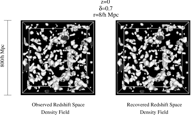
Figure 3: A comparison of the smoothed redshift space density fields of the output of the resolution simulation described in the text, and the reconstructed field based on those observations. A contour of $\delta=0.7$, smoothed with a Gaussian filter of $r=8h^{-1}$ Mpc is shown. Note the high level of agreement between structures in the true and reconstructed fields.

In Figure 3 we show a density contour of $\delta=0.7$ for the observed redshift space density field, smoothed with a Gaussian filter with a radius of $8h^{-1}$ Mpc, and a similar plot, but for the field resulting from our PLA reconstruction. Recall that the underlying particle field for the latter is based on running the reconstructed initial conditions through a PM code and taking the smoothed density field. A visual inspection demonstrates that the two fields are virtually identical.

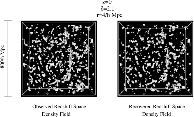
Figure 4: As in the previous figure, but with a Gaussian smoothing radius of $4h^{-1}$ Mpc, and a density contour of $\delta=2.1$.

We plot a similar comparison in Figure 4, except with a smoothing radius of only $4h^{-1}$ Mpc, and a density contour of $\delta=2.1$. On these scales, too, the fields are very similar. The reconstructed field, however, seems to differ somewhat on small scales. If we had an a priori model of the power spectrum, this small scale power could be suppressed numerically.

More quantitatively, Figure 5 shows the fit between the reconstructed and true field as a function of scale. Narayanan & Croft (1999) provide the goodness of fit metric:

$$\Delta^{2}(k,t)=\frac{\sum[\delta_{1}({\bf k})-\delta_{2}({\bf k})]^{2}}{\sum[\delta_{1}({\bf k})^{2}+\delta_{2}({\bf k})]^{2}}\ .$$ (32)

In this case, $\delta_{1}({\bf k})$ and $\delta_{2}({\bf k})$ are the Fourier transforms of the true and reconstructed redshift density fields. For perfect matching on a particular scale, this metric goes to zero. For uncorrelated fields, it goes to one.

As Figure 5 illustrates, the fit for all four comparisons is very good even into the nonlinear regime ($k\simeq 0.4h\ {\rm Mpc}^{-1}$). The best fit was found for the final conditions in redshift space, since this was the actual set of observations to be matched. However, it is shown that the real space field at z=0 is also reconstructed quite well, as are the corresponding initial conditions. In particular, the relevant scale is that for which $\Delta^{2}=0.5$ for each comparison. In this case, the real and redshift initial conditions are well matched down to a scale of $18.6$ and $19.5h^{-1}$ Mpc, respectively, and the real and redshift space final conditions are matched down to scales of $15.1$ and $12.7h^{-1}$ Mpc, respectively.

Another measure of the quality of the reconstruction is the isotropy of the reconstructed real space density field. We may do this by decomposing the power spectrum of the field into Legendre Polynomials (e.g. Hamilton, 1992):

$$P({\bf k})=\sum_{l\ {\rm even}}{\cal P}_{l}(\mu)P_{l}(k)\ ,$$ (33)

where $\mu$ is the cosine of the angle between the direction vector, ${\bf k}$, and the line of sight, ${\cal P}_{l}(\mu)$ are the Legendre polynomials, $P_{l}(k)$ are the azimuthally-averaged multipole expansion of the power spectrum. Taking the inverse Legendre transform, we find (Cole, Fisher and Weinberg 1995):

$$P_{l}(k)=\frac{2l+1}{4\pi}\int_{-1}^{1}d\mu\int_{0}^{2\pi}d\phi P({\bf k}){\cal P}_{l}(\mu)\ .$$ (34)

Here, we will only be using the monopole and quadrupole moments, which, as a reminder are ${\cal P}_{0}(\mu)=1$ and ${\cal P}_{2}(\mu)=(3\mu^{2}-1)/2$. We may thus measure the isotropy of the distribution by computing the ratio:

$$Q_{x}(k)\equiv\frac{P_{2}(k)}{P_{0}(k)}\ .$$ (35)

Since the real universe is isotropic, an accurately computed reconstruction should have a quadrupole equal to zero on all scales.

Figure 6 shows the quadrupole ratio as a function of scale for both 1 and 2 iterations. Two things are clear from this plot, however. First, the overall isotropy does improve with additional iterations. Secondly, there is a systematic effect in generating these anisotropies which is almost certainly caused by an anisotropic noise term. In the appendix, we use the quadrupole and hexadecipole moments to illustrate that this effect is dominated by noise, rather than by a systematic underestimate of the radial velocity term, for example.

This noise term comes out of the reconstruction scheme, itself. In the previous section, we discussed how one goes about approximately rewinding the trajectory of a particle in order to determine its initial constraint. However, there was an assumption that linearity approximately held. As structure gets more and more nonlinear, this assumption will fail to hold, and the particle matching technique will break down. Future advances in reconstruction methods will have to take this into account. It may be possible to apply PLA in an iterative and statistical way in order better do this matching.

4 Applications: Breaking the Bias Degeneracy

4.1 Motivation

Though the reconstruction of nonlinear fields is interesting in its own right, we have begin this investigation into redshift space for the purpose of finding out something about cosmology. As a motivation for this sort of reconstruction analysis of redshift surveys, we address the $\Omega_{M}$-$b$ degeneracy in redshift surveys, and discuss how the degeneracy might be broken without recourse to outside dynamical estimates of $\Omega_{M}$. We will test the effectiveness of using PLA to break the degeneracy.

We begin by introducing the problem as it appears in the linear regime. Excellent recent reviews of this topic is given by Hamilton (1998) and by Strauss & Willick (1995), and we will therefore present only an overview of the linear biasing problem.

Let us first suppose that we have the full velocity field information about a group of almost uniformly distributed particles. Let us further suppose that these particles are biased with respect to some true underlying CDM field, such that:

$$\delta_{g}({\bf x},t_{0})=b\delta({\bf x},t_{0})\ ,$$ (36)

where the unsubscripted $\delta$ is the CDM density field, and $\delta_{g}$ (for galaxies) represents the density field of some biased tracer of the mass. Note that a straight linear biasing model may be replaced with any deterministic, local, and monotonically increasing function of $\delta({\bf x},t_{0})$ without changing the essence of the discussion or the biasing problem in general. Blanton (1999) provides an excellent review of various types of biasing models.

With linear bias greater than unity the velocity field is of lower amplitude than one would directly infer from a measurement of $\delta_{g}$. From (36), equation (6) may be replaced by:

$$\nabla\cdot{\bf v}({\bf x},t_{0})=-\beta\delta_{g}({\bf x},t_{0})\ ,$$ (37)

where

$$\beta\equiv\frac{f(\Omega_{M},\Omega_{\Lambda},t_{0})}{b}\simeq\frac{\Omega_{M}^{0.6}}{b}$$ (38)

and

$${\bf v}=f(\Omega_{M},\Omega_{\Lambda},t_{0})\ {\bf p}\ .$$ (39)

Thus, the divergence of the velocity field and density field are related by the same proportionality constants for all combinations of $\Omega_{M}$ and $b$ which yield the same $\beta$. This is the crux of the degeneracy problem.

In a redshift survey, we do not actually know the divergence of the velocity field, but rather must infer it through anisotropies in the redshift density field. Kaiser (1987) shows that in the linear regime, there is a straightforward relationship between the real and redshift space density fields in k-space in the d.o.a.:

$$\delta^{s}_{g}({\bf k})=\hat{\bf S}\delta^{x}=\delta^{x}({\bf k})[1+\beta\mu^{2}]\ ,$$ (40)

where $\hat{\bf S}$ is the linear redshift distortion operator, $\delta^{s}_{g}({\bf k})$ is the Fourier transform of the galaxy density field in redshift space, and $\delta^{x}({\bf k})$ is the Fourier transform of the underlying CDM density field in real space.

From this relationship, a redshift space power spectrum field may be compared to the real space power spectrum:

$$P_{g}^{s}({\bf k})\equiv|\delta^{s}_{g}({\bf k})|^{2}=P({\bf k})[1+\beta\mu^{2}]^{2}\ .$$ (41)

We can further decompose the power spectrum field into Legendre polynomials (equation 33; Hamilton 1992). We then take the inverse Legendre transform (equation 34; Cole, Fisher and Weinberg 1995) and compute the quadrupole moment.

Taking the Legendre expansion of the form of the linear density field (equation 33) above, we find that the moments of the biased, redshift space distribution may be related to the underlying real space distribution as follows (Hamilton 1998):

$$P^{s}_{g,0}(k) = \left(1+\frac{2}{3}\beta+\frac{1}{5}\beta^{2}\right)P(k)$$ (42)

$$P^{s}_{g,2}(k) = \left(\frac{4}{3}\beta+\frac{4}{7}\beta^{2}\right)P(k)\ .$$ (43)

Though the underlying power spectrum is not known, this quadrupole ratio may be computed as:

$$Q_{s}(k)\equiv\frac{P^{s}_{g,2}(k)}{P^{s}_{g,0}(k)}=\frac{\frac{4}{3}\beta+\frac{4}{7}\beta^{2}}{1+\frac{2}{3}\beta+\frac{1}{5}\beta^{2}}\ .$$ (44)

Since the multipole expansion may be computed directly from the observed redshift space density field, it is clear that in the linear regime, the quadrupole ratio is degenerate for a particular value of $\beta$.

In addition, $\beta$ may be estimated through the use of distance-velocity comparisons. In practice, measurements of $\beta$ are still quite difficult due to the noisy data involved. Willick (2000) gives a review of current estimates, and finds a value of $\beta=0.5\pm 0.04$ from the IRAS velocity field and the Mark III Catalog used to estimate distances. This is relatively unchanged from the earlier estimate based on measured redshift-space anisotropy by Cole, Fisher, & Weinberg (1995) of $\beta=0.54\pm 0.3$. Ballinger et al. (2000) estimate $\beta=0.4\pm 0.1$ for the IRAS 0.6 Jy PSCz survey from analysis of anisotropies. Similar values are found from the Optical Redshift Survey catalog (Baker et al. 1998).

After estimating $\beta$, how does one estimate $\Omega_{M}$ without recourse to direct mass estimates? We answer this by first pointing out that a correctly reconstructed real space density field will be perfectly isotropic. That is, $Q_{x}(k)=0$ on all scales. Nonlinearities is the evolution of the density field will mean that the linear redshift distortion operator will no longer be valid on all scales. By reconstructing fields using PLA for different combinations of $\Omega_{M}$ and $b$, and measuring the quadrupole moment for the reconstructed field, we can determine the “true” cosmology as that which minimizes the anisotropy.

4.2 Simulations

4.2.1 Constraining Bias

In order to test this approach, we have run two simulations, each extending only into the mildly nonlinear regime. We have found that simulations which contain highly nonlinear structure do not effectively differentiate between different cosmologies due to the excessive noise and difficulty of doing the particle matching on small scales.

The two simulations were each run with $\beta=0.5$ and a boxsize of $L=1000h^{-1}$ Mpc, the first with $\Omega_{M}=0.3$, $\Omega_{\Lambda}=0.7$, and $b=1$, and the second with $\Omega_{M}=1$, $\Omega_{\Lambda}=0$, and $b=2$. Each simulation was run with $64^{3}$ particles, and $128^{3}$ gridcells, and the PLA reconstruction used 4 basis functions. The “observations” of these simulations were the redshift-space density fields in the d.o.a. After reconstructing the initial density field for a particular assumed bias, we ran the initial conditions through a PM code, and measured the quadrupole moment in real-space, where it should vanish. The “mean” quadrupole moment is estimated as:

$$\langle Q_{x}^{2}\rangle=\frac{\int dk\ Q^{2}_{x}(k)\ k^{2}\ e^{-k/k_{l}}}{\int dk\ k^{2}\ e^{-k/k_{l}}}\ ,$$ (45)

where $k_{l}$ is a limiting scale at which point grid and/or nonlinear effects will become important. We have assumed $k_{l}=20\times 2\pi/L_{box}$, but found similar results for $k_{l}=\infty$. The peak of this contribution occurs around $3k_{l}$, or on a physical scale of $\sim 16h^{-1}$ Mpc, the nonlinear scale. The results of each model tested are shown in Figure 7 for the $\Omega_{M}=0.3$ simulation, and Figure 8 for the $\Omega_{M}=1$ simulation.

In each case, we find that the best fit value of $\Omega_{M}$ corresponds to the actual value of $\Omega_{M}$ used in the simulation. That is, by tracing the detailed evolution of a mildly nonlinear field, PLA can effectively break the $\beta$ degeneracy.

In estimating this effect from a real survey, we would have to Monte Carlo observations based on the survey geometry, selection function, and the like, in order to estimate $\Omega_{M}$ and its errors. While direct error estimation is difficult with only two realizations, the results are quite suggestive that this will be an effective way to constrain $\Omega_{M}$ directly. Susperregi (2000) uses an Eulerian least action code to similarly show that the bias degeneracy may be broken through accurate reconstruction.

As a final test of PLA as a redshift space reconstruction scheme, we show that one may obtain somewhat better estimates of $\beta$, itself, from the assumed isotropy of the reconstructed real space density field than from the redshift space anisotropy. This is illustrated in Figure 9, in which we show a comparison between $Q_{x}(k)$ of the reconstructed field for simulation 1, assuming the correct value of $\Omega_{M}=0.3$, and the corresponding quadrupole moment residuals, $Q_{s}(k)-Q_{s}^{L}$ of the observed redshift space field. Note that the term $Q_{s}^{L}$ is simply that which one would estimate from an assumption of the correct value of $\beta$.

On large scales, these two statistics are almost identical. However, on smaller scales, when nonlinearities begin to become important, the two statistics both exhibit anisotropies. The redshift space field, however, becomes anisotropic on larger scales. Since the corresponding uncertainties in $\beta$ are approximately proportional to one over the square root of the number of modes probed, we may relate the expected uncertainties from the reconstructed field to that from the redshift field as:

$$\frac{\sigma_{\beta}^{PLA}}{\sigma_{\beta}^{Z}}\simeq\frac{\sigma_{Q}^{PLA}\frac{\partial\beta}{\partial Q^{PLA}}(k^{PLA}_{{\rm max}})^{-3/2}}{\sigma_{Q}^{Z}\frac{\partial\beta}{\partial Q^{Z}}(k^{Z}_{{\rm max}})^{-3/2}}\ ,$$ (46)

where the superscript “Z” refers to the estimate from the redshift space field and the superscript “PLA” refers to the estimate from the reconstructed real space field. For $\Omega_{M}=0.3$, all of the partial derivatives are almost exactly one. Moreover, estimates of the scatter in the quadrupole estimates show that $\sigma_{\beta}^{PLA}\simeq 0.9\sigma_{\beta}^{Z}$. Finally, since Figure 9 shows $k^{PLA}_{{\rm max}}\simeq 1.25k^{Z}_{{\rm max}}$, the approximate relation between the uncertainty in the bias between the two errors is $\sigma_{\beta}^{PLA}\simeq 0.65\sigma_{\beta}^{Z}$. Thus, we are able to generate a somewhat better constrained estimate of $\beta$ from the reconstructed density field, as compared to the observed field.

5 Future Prospects

This paper has discussed the problem of reconstructing the underlying real space CDM density field and its evolution from galaxy redshift surveys under rather idealized conditions. We have assumed full sampling, a constant linear bias relation with no morphological segregation, the distant observer approximation, no errors in measurement, and a very regular geometry. We have shown that theoretically even a mildly nonlinear field can be reconstructed using PLA to break the bias degeneracy. In actual observations almost none of these assumptions will hold. We would like to end this work with a brief discussion of how these effects might be appropriately modeled, and mention a few possible candidates of real surveys to which the PLA method might be applied.

Throughout, we have assumed a cubic geometry. In simulating a realistic survey, a mask must be applied such that statistics may be correctly computed for the true survey volume. Additionally, for many observational samples of interest, the distant observer approximation no longer describes the system adequately. Over the course of its lifetime, a galaxy may have traversed a significant angle in the sky, making the use of Cartesian coordinates difficult. An obvious solution to this problem is to write the PLA equations in spherical coordinates.

An additional concern in the application of PLA to realistic observations is that the biasing model that we have used here is a strictly linear one, and observational evidence suggest that biasing may be much more complex (e.g. Blanton 1999 and references therein). In fact, we have only used linear bias in this work for its simplicity. PLA would be applicable to any model of deterministic bias, even one which had an explicit model of morphological segregation. It is not clear how one might effectively reconstruct a field under the assumption of a significantly stochastic bias model.

Even under the simplest of approximations, realistic surveys are not cubic, not necessarily contiguous, and generally have nonuniform selection functions. The issues of contiguity and geometry are related, in that in both we need to approximate the density field outside the survey volume in order to correctly estimate the potential field within.

Lahav et al. (1994) apply one such technique to the IRAS 1.2 Jy survey (Strauss et al. 1992; Fisher et al. 1995) in which expansion of the density field in spherical harmonics is used to reconstruct the field outside the survey volume. In essence, this is very similar to assuming a particular autocorrelation function, and generating an outside field based on a truncated form of that function and the observed field near the edges. In many respects, this is quite similar to the sort of reconstruction done using the “Constrained Initial Conditions” technique by Hoffman & Ribak (1991,1992), since both use observed the observed autocorrelation function to build realistic external fields around observed structure.

The final issue in real surveys concerns non-uniformity and noise within the survey volume. However, for flux limited surveys such as the IRAS 1.2 Jy and PSCz (Saunder et al. 2000) surveys, at large distances, shot noise begins to dominate calculations of the density field. Since the observed density field is derived from an incomplete sampling of a finite number of discrete points, the uncertainties in the observed density field behaves like a Poisson statistic, with $\sigma\propto 1/\sqrt{N_{gal}}$. In order to correctly anticipate the effects of shot noise when running simulations of a particular survey, a random component needs to be added to the observed density field.

Moreover, a non-uniform selection function, coupled with observations in redshift space results in Malmquist bias. That is, the “true” selection function is based on observed fluxes, and hence is a function in real space. The observations, however, are of densities in redshift space. Strauss & Willick (1995) give an excellent review of how these issues are dealt with in reconstructing density fields.

These considerations are all with an eye toward learning about cosmology from redshift surveys. For example, the IRAS 0.6 Jy PSCz Survey (Saunders et al. 2000) is an especially promising recent candidate for analysis, as it is publicly available and has nearly full sky coverage. Hamilton, Tegmark, & Padmanabhan (2000) have already estimated $\beta=0.41^{+.13}_{-.12}$ from this survey, and Ballinger et al. (2000) find a similar result of $\beta=0.4\pm 0.1$. Both methods used only linear theory, however. Valentine, Saunders, & Taylor (2000) do a somewhat higher order reconstruction, by using the PIZA method, and find a best fit to the survey with a slightly higher value of $\beta\simeq 0.5$. In testing our code, we have found that one can get a better measure of $\beta$ by using PLA to reconstruct a density field under some fiducial cosmology, and comparing cosmologies to see which produce the minimum anisotropy in the real space field. We have showed that ideally, PLA can be used to discriminate between “degenerate” pairs of bias and $\Omega_{M}$. Finally, we showed that PLA produces a means by which uncertainties in the measurement of $\beta$ itself can be reduced.

Another interesting prospect is the application to PLA to large distance redshift surveys, since one of the byproducts of PLA is the real space density field. Nusser et al. (2000) use the $D_{n}-\sigma$ relation of the ENEAR redshift-distance survey (da Costa et al. 2000) as test particles within the PSCz survey, much as we would wish to do using PLA. A reconstruction was done using the method described by Nusser & Davis (1995). Predicted distances from the reconstructed field can then be compared with the estimated distances from the ENEAR survey. They also estimated $\beta\simeq 0.5$.

While the PSCz survey contains $\sim 15,000$ redshifts, the current generation of redshift surveys is producing an even greater opportunity to measure statistical and global properties of the universe. When complete, the SDSS redshift survey (York et al. 2000), will produce $\sim 10^{6}$ galaxy redshifts, and will cover a quarter of the sky out to Petrosian magnitude, $r_{p}^{\prime}=17.7$ to $z\simeq 0.15$. The 2dF survey (Colless 1999) will ultimately measure redshifts over a quarter of a million galaxies, out to $b_{J}=19.5$.

Reconstruction of fields from these enormous datasets will prove a significant computational challenge. However, it is well worth it, as PLA can yield insight into the underlying power spectrum, bias, and cosmological parameters.

Appendix A The Effects of Noise on Multipole Moments

In §3, we found that the reconstructed real space density field of the high-resolution simulation had a significant and seemingly systematic quadrupole moment at small scales. The question which arises out of this is, does this quadrupole represent a systematic error in the reconstruction along the line of sight (such as would occur, for example, if the assumed value of $\beta$ were incorrect), or does it represent a stochastic term?

To examine this question, let us consider the following form of a reconstructed field with a very simple error term:

$$\tilde{\delta}({\bf k})=\delta({\bf k})\left[1+\mu^{2}B({\bf k})+\mu^{2}\epsilon({\bf k})\right]\ ,$$ (A1)

where ${\bf k}$ is a Fourier space component, $\delta({\bf k})$ is the true real space field we are attempting to reconstruct, $\tilde{\delta}({\bf k})$ is the reconstructed form of the field, $\mu^{2}$ is the cosine of the angle between the ${\bf k}$ and the line of sight, $B$ is a systematic, “bias” term, and $\epsilon({\bf k^{2}})$ is an anisotropic random error drawn from a $N(0,\sigma^{2}({\bf k}))$ distribution.

If the corresponding real space density field of redshift space observations have been perfectly reconstructed and contain no noise, the reconstructed field is simply equal to the true underlying field, and thus will be perfectly isotropic in $k$-space. However, let us imagine that a field contains no noise, but the reconstruction is such that we have assumed that $\tilde{\delta}({\bf k})=\delta_{s}({\bf k})$, or the real space density field is the same as the redshift space field. Under those circumstances, $B({\bf k})=\beta$, hence our terminology.

Finally, let us consider a more general case, one in which we wish to test for a systematic form of $B({\bf k})$ and for the existence of a random noise component. In that case, the reconstructed three-dimensional power spectrum may be written as:

$$\left<\frac{\tilde{P}({\bf k})}{P({\bf k})}\right>=1+2\mu^{2}B({\bf k})^{2}+\mu^{4}B({\bf k})^{2}+\mu^{4}\sigma^{2}({\bf k})$$ (A2)

If we then decompose these terms into multipole moments (see §5.4.1) and assume that the noise and systematic terms are simply scale dependent, we find:

$$\tilde{P}_{0}(k) = P(k)\left[1+\frac{2}{3}B(k)+\frac{1}{5}B(k)^{2}+\frac{1}{5}\sigma^{2}(k)\right]$$ (A3)

$$\tilde{P}_{2}(k) = P(k)\left[\frac{4}{3}B(k)+\frac{4}{7}B(k)^{2}+\frac{4}{7}\sigma^{2}(k)\right]$$ (A4)

$$\tilde{P}_{4}(k) = P(k)\left[\frac{8}{35}B(k)^{2}+\frac{8}{35}\sigma^{2}(k)\right]$$ (A5)

We may then look at the relationship between the quadrupole ratio, $\tilde{Q}(k)\equiv\tilde{P}_{2}(k)/\tilde{P}_{0}(k)$ and the hexadecipole ratio, $\tilde{H}(k)\equiv\tilde{P}_{4}(k)/\tilde{P}_{0}(k)$. We have two extremes. In the case of no anistropic noise component, each ratio is simply a parametric function of $B(k)$, and thus, a straightforward relation between the two may be plotted.

If, on the other hand, the anisotropic noise term dominates, we find the relation:

$$\tilde{H}^{NOISE}(k)=\frac{2}{5}\tilde{Q}^{NOISE}(k)\ .$$ (A6)

We illustrate this in Figure 10. We show that for an observed redshift density field, the deterministic bias term dominates. Though we do not necessarily have the correct form of the anisotropic error term, this error which would seem to be at the root of the systematic small scale quadrupole in the high-resolution simulation.

Since we may take as a prior that the universe is inherently isotropic, regularization or iterative techniques might be employed in future reconstruction schemes which explicitly find a fully isotropic real space solution.

Figure 1: A simulation of a quasi-linear Zel’dovich pancake. In each panel, the solid lines show the “true” real- and redshift space density fields before and after running the corresponding particles through an N-body code. Panels a) and b) show the initial density fields in redshift and real space, respectively. The long-dashed lines represent the initial density field computed by using PLA. Panel c) shows the evolved field in real space. The solid line shows the true field, while the dotted line shows the first estimate of the field from the redshift space distribution, and the short dashed line shows the converged value. The long dashed line shows the density field computed using PLA. Panel d) shows the evolved field in redshift space. The dotted line denotes the density field corresponding to the redshift positions generated by using the laminar flow density matching method described in the text. The long dashed line shows the density field computed by using PLA.

Figure 2: The real space-redshift space coordinate relationship for a Zel’dovich pancake. The solid line shows the relationship as given by the output of an N-body simulation. The squares show the relation as given by the VELMOD-like scheme used to approximate the real-space density field. Finally, the solid points show the output from PLA.

Figure 5: The Fourier difference statistic for the high resolution simulation. This compares the true initial and final conditions in real and redshift space to those generated by using the reconstruction scheme using only the observations of the final redshift space density field. The dotted line shows the first iteration of PLA, and the solid line, an additional iteration. Note that a physical scale of $16h^{-1}{\rm Mpc}$ (the nonlinear scale) occurs at $\log_{10}(k)=-0.4$.

Figure 6: The quadrupole moment ratio as a function of $|k|$ for the reconstructed high-resolution real space density field simulation. Solid squares represent the results from one iteration of PLA, while solid circles are the results from a second iteration.

Figure 7: The weighted-average real space quadrupole ratio for the reconstructed density fields with various assumed cosmologies in the $\Omega_{M}=0.3$ simulation. Note that the quadrupole ratio is minimized for $\Omega_{M}=0.3$, indicating that PLA reconstruction effectively breaks the $\beta$ degeneracy.

Figure 8: As in the previous figure, but for the $\Omega_{M}=1$ simulation. Here, the quadrupole ratio is minimized for $\Omega_{M}=1$, again indicating the reconstruction method has broken the degeneracy.

Figure 9: A comparison of the scale dependent quadrupole moment ratio for the reconstructed real space density (filled circles), and the “observed” redshift space density (open squares), with the linear quadrupole term subtracted. Each estimate was done using the $\Omega_{M}=0.3$ low resolution simulation. Note that while both statistics are approximately zero at large scales, there is a systematic divergence at small scales. This turnoff occurs at larger scales for the direct redshift estimate than for the estimate based on the reconstructed field.

Figure 10: Scatter plots relating the quadrupole and hexadicpole ratios in the high-resolution simulations discussion in §3. The solid line shows the expected relation for a systematic anisotropy (the $\beta$-like term), while the dashed line shows the expected relation for our simplified anisotropic noise model. Panel a) shows the ratios as observed in the redshift space density field. Note that the systematic effect dominates, since the anisotropies are completely due to redshift space distortions. Panel b) shows the ratios for the reconstructed field. The hexadecipole ratio is much higher than what would be expected from a deterministic effect.

References

- (1) Baker, J. E., Davis, M., Strauss, M. A., Lahav, O. & Santiago, B. X. 1998, ApJ, 508, 6
- (2) Ballinger, W.E., Taylor, A.N., Heavens, A.F., & Tadros, H. 2000, astro-ph/0005094
- (3) Bardeen, J., Bond, J.R., Kaiser, N., & Szalay, A. 1986, ApJ, 304, 15
- (4) Bernardeau, F. 1992, ApJL 390, 61
- (5) Bertschinger, E. & Dekel, A. 1989, ApJ, 336, L5
- (6) Blanton, M., 1999, Ph.D. Thesis, Princeton University, available at http://www-astro-theory.fnal.gov/Personal/blanton/thesis/index.html
- (7) Blanton, M. 2000, submitted to ApJ
- (8) Chodorowski, M. J. 2000, submitted to MNRAS
- (9) Chodorowski, M. J. Łokas, E. L., Pollo, A., & Nusser, A. 1998, MNRAS 300, 1027
- (10) Chodorowski, M. J. & Łokas, E. L. 1997, MNRAS 287, 591
- (11) Cole, S., Fisher, K.B., & Weinberg, D.H. 1995, ApJ 275, 515
- (12) Colless, M. 1999, Phil. Trans. R Soc. Lond. A, 357, 105
- (13) da Costa, L.N., Bernardi, M., Alonso, M.V., Wegner, G., Willmer, C.N.A., Pellegrini, P.S., Rite, C. & Maia, M.A.G. 2000, AJ, in press
- (14) Davis, M., Efstathiou, G, Frenk, C.S., & White, S.D.M. 1985, ApJ, 292, 371
- (15) Davis, M. & Geller, M.J. 1976, ApJ, 208,13
- (16) Dekel, A., Bertschinger, E., & Faber, S.M. 1990, ApJ, 364, 349
- (17) Dekel, A., Eldar, A., Kolatt, T., Yahil, A., Willick, J. A., Faber, S. M., Courteau, S., & Burstein, D. 199, ApJ. 522, 1
- (18) Hamilton, A.J., Tegmark, M., & Padmanabhan, N. 2000, submitted to MNRAS
- (19) Dekel, A. & Lahav, O. 1999, ApJ 520, 24
- (20) Fisher, K.B., Huchra, J.P., Strauss, M. A., Davis, M., Yahil, A. & Schlegel, D. 1995, ApJS, 100, 69
- (21) Giavalisco, M., Mancinelli, B., Mancinelli, P.J., & Yahil, A. 1993, ApJ, 411, 9
- (22) Goldberg, D.M. & Spergel, D.N. 2000, ApJ, in press
- (23) Hamilton, A.J.S., 1992, ApJ, 385, L8
- (24) Hamilton, A.J.S., 1998, “The Evolving Universe. Selected Topics on Large-Scale Structure and on the Properties of Galaxies,” ed. Hamilton, D., p. 185.
- (25) Hatton, S. & Cole, S. 1998, MNRAS, 296, 10
- (26) Hockney, R.W. & Eastwood, J.W. 1981, “Computer Simulations Using Particles” (New York: McGraw Hill)
- (27) Hoffman, Y. & Ribak, E. 1991, ApJ, 380, L5
- (28) Hoffman, Y. & Ribak, E. 1992, ApJ, 394, 448
- (29) Hubble, E.P. 1936, “The Realm of the Nebulae,” (New Haven: Yale University Press)
- (30) Kaiser, N. 1984, ApJ, 284, L9
- (31) Kaiser, N. 1987, MNRAS, 227, 1
- (32) Kudlicki, A., Chodorowski, M., Plewa, T., & Różyczka, 1999, submitted to MNRAS
- (33) Lahav, O., Fisher, K.B., Hoffman, Y., Scharf, C.A. & Zaroubi, S., 1994, ApJL, 423, L93
- (34) Narayanan, V.K. & Croft, R.A.C. 1999, ApJ 515, 471
- (35) Nusser, A. & Davis, 1994, ApJ, 421, L1
- (36) Nusser, A. & Davis, 1995, MNRAS, 276, 1391
- (37) Nusser, A., da Costa, L.N., Branchini, E., Bernardi, M., Alonso, M.V., Wegner, G., Willmer, C.N.A., & Pellegrini, P.S. 2000, submitted to MNRAS
- (38) Nusser, A., Dekel, A., Bertschinger, E., & Blumenthal, G.R. 1991, ApJ, 379, 6
- (39) Oemler, A. 1974, ApJ, 194, 1
- (40) Peebles, P. J. E. 1980, “The Large-Scale Structure of the Universe” (Princeton: Princeton University Press)
- (41) Peebles, P.J.E. 1989, ApJ, 344,L53
- (42) Press, W.H., Teukolsky, S.A., Vetterling, W.T., & Flannery, B.P. 1992 “Numerical Recipes: The Art of Scientific Computing” (Cambridge, England: Cambridge University Press)
- (43) Sahni, V. & Coles, P. 1995, Phys. Rep.
- (44) Santiago, B.X., & Strauss, M.A. 1992, ApJ, 387, 9
- (45) Saunders, W. Sutherland, W.J, Keebles, O., Oliver, S.J., Rowan-Robinson, M., McMahon, R.G., Efstathiou, G.P., Tadros, H., White, S.D.M., Frenk, C.S., Carramiñana, A., & Hawkins, M.R.S. 2000, MNRAS, accepted
- (46) Schmoldt, I. M. & Saha, P. 1998, AJ 115, 2231
- (47) Sigad, Y., Eldar, A., Dekel, A., Strauss, M. A. & Yahil, A. 1998, Apj 495, 516
- (48) Strauss, M.A. & Willick, J. A. 1995, Phys. Rep., 261, 271
- (49) Strauss, M. A., Yahil, A., Davis, M., Huchra, J.P. & Fisher, K. 1992, ApJ, 397, 395
- (50) Susperregi, M. & Binney, J. 1994, MNRAS 271, 719
- (51) Susperregi, M. 2000, submitted to ApJ, astro-ph/0002369
- (52) Valentine, H., Saunders, W., & Taylor, A. 2000, submitted to MNRAS
- (53) Willick, J. A., 2000, “Proceedings of the XXXVth Rencontres de Moriond: Energy Densities in the Universe.”
- (54) Willick, J. A., Strauss, M. A., Dekel, A. & Kolatt, T. 1997, ApJ 486, 629
- (55) York et al. 2000, AJ, accepted, preprint at http://xxx.lanl.gov/abs/astro-ph/0006396
- (56) Zaroubi, S. & Hoffman, Y. 1996, ApJ 462, 25
- (57) Zel’dovich, Y.B. 1970, A&A, 5, 84