Cosmic concordance and the fine structure constant

Abstract

Recent measurements of a peak in the angular power spectrum of the cosmic microwave background appear to suggest that geometry of the universe is close to being flat. But if other accepted indicators of cosmological parameters are also correct then the best fit model is marginally closed, with the peak in the spectrum at larger scales than in a flat universe. Such observations can be reconciled with a flat universe if the fine structure constant had a lower value at earlier times, which would delay the recombination of electrons and protons and also act to suppress secondary oscillations as observed. We discuss evidence for a few percent increase in the fine structure constant between the time of recombination and the present.

I Introduction

Cosmologists have for many years struggled to find a model of the universe consistent with all the available evidence. Recently, many observations have pointed to the universe being spatially flat with cold dark matter (CDM) making up approximately a third of the critical density, and the remainder dominated by a component with a negative equation of state such as a cosmological constant, $\Lambda$. This confluence of evidence, which includes measurements of the expansion and acceleration of the universe, bounds on the age of the universe, and constraints from large scale structure and galaxy clusters, has been called ‘cosmic concordance’ [1].

The restriction to spatially flat models was originally motivated by theoretical arguments, in particular to be consistent with inflationary models of the early universe. However, measurements of the anisotropy in the cosmic microwave background (CMB) have given strong observational support to this assumption. The position of the first Doppler peak in the CMB power spectrum is sensitive to the spatial geometry and the epoch of last scattering of the CMB photons relative to the present age of the universe[2]. Recent measurements by the balloon borne detectors BOOMERanG[3] (B98) and MAXIMA[4] (M99) indicate an increase in power at angular scales of approximately two degrees, very close to the expected position of the first Doppler peak in spatially flat models.

While providing tentative confirmation of a flat universe, the new data has also raised many questions as to the precise viability of the concordance[5, 6, 7, 8]. In particular, the position of the first peak as detected by BOOMERanG ($\ell_{\rm peak}=197\pm 6$) appears to be at slightly larger scales than expected in generic flat models — a conclusion which is only slightly weakened by the inclusion the less sensitive MAXIMA data [9]. In addition, both data sets indicate secondary Doppler peaks that are much less pronounced than expected in models compatible with primordial Big Bang Nucleosynthesis (BBN) [10, 11]. There are, of course, numerous possible explanations for these discrepancies. For example, the shift of the peak to larger scales could indicate a universe which is slightly closed [6, 8], while the suppression of the second peak could be evidence that the baryon density is higher than has been indicated by BBN[7, 8]. However, these solutions require either giving up the elegance of spatially flat models or run into direct conflict with other cosmological measurements, particularly those related to BBN.

Another possible solution which addresses both unexpected features of the data is to delay the epoch of last scattering. This would increase the size of the sound horizon at last scattering and shift the first peak to larger scales while keeping a spatially flat universe. It would also simultaneously increase the density of baryons relative to that of the photons during the epoch of last scattering, suppressing the amplitude of the second peak. Within the standard framework, it is rather difficult to change the time of decoupling since it would require a mechanism, astrophysical [12] or otherwise [13, 14, 15], which could delay the formation of neutral hydrogen. Peebles et al. [12] suggested that non-linear structures at extremely high redshift could act as a source for Lyman-$\alpha$ photons which photo-ionize the hydrogen. However, this is very unlikely in standard adiabatic models for structure formation, though it is a possibility if the initial fluctuations were non-Gaussian.

In this paper, we focus on another possible mechanism for delaying photon decoupling: that the electrons and protons might have been more weakly bound at high redshifts than they are today. In particular, we consider whether the observations contain evidence for a running of the fine structure constant, $\alpha=e^{2}/(4\pi\hbar c)$, between the time of recombination, where the CMB last scattered, and the present epoch. Changes in $\alpha$ modify the parameters governing recombination [16, 17], which, depending on the sign, can lead to early ($\delta\alpha(t_{\rm rec})=\Delta\alpha(t_{\rm rec})/\alpha>0$) or delayed ($\delta\alpha(t_{\rm rec})<0$) recombination. Here, we have defined $\Delta(t)=\alpha(t)-\alpha(t_{0})$, where $t$ is cosmic time and we denote $t_{0}$, $t_{\rm rec}$ and $t_{\rm nuc}$ throughout as the times of the present day, recombination and nucleosynthesis respectively.

Such variation of physical constants has been the subject of much attention, both observational and theoretical, in recent years. The theoretical motivation comes from String or M-theory in models where there are compact extra dimensions. These extra dimensions may have either stabilized before recombination ($\delta\alpha(t_{\rm rec})=0$) or they may still be rolling down their potential, causing all the coupling constants to vary ($\delta\alpha(t_{\rm rec})\neq 0$). The standard way in which to do this is using a scalar field known as the dilaton, but no stabilizing potential has ever been derived from anything which could be described as a candidate fundamental theory; all proposed stabilizing mechanisms appear to be ad hoc. Slow variation in $\alpha$ could, therefore, be considered at some level as a prediction of fundamental theory. It has also been pointed out [18, 19] that models in which $\alpha$ varies can be thought of as models with a varying speed of light [20, 21].

Of course, limits exist on changes in $\alpha$ due to various terrestrial, astrophysical and cosmological arguments. Terrestrial limits come primarily from elements which have long-lived $\beta$ decay, atomic clocks and the OKLO natural nuclear reactor [22], for which the limit is $-0.9\times 10^{-7}<\delta\alpha<1.2\times 10^{-7}$ over a time period of around 1.8 billion years, although this is model and theory dependent since the limits are sensitive to possible simultaneous variations in other coupling constants. Cosmological limits come from the Helium abundance in BBN and quoted limits can be expressed roughly as $|\delta\alpha(t_{\rm nuc})|<10^{-2}-10^{-4}$ [23, 24, 25] at $z\approx 10^{9}-10^{10}$, although this is again highly model dependent; we shall return this issue in a detailed discussion below. Astrophysical limits arise from systems which absorb quasar emissions over a wide redshift range of $z\sim 0.1-3$ [26]. After many years of deriving upper bounds on $\delta\alpha$, a statistical detection of $\delta\alpha=(-1.1\pm 0.4)\times 10^{-5}$ has been claimed recently [27] due to measurements of relativistic fine structure in absorption systems in the range $0.6<z<1.6$, with more data soon to be published.

In what follows we will work within the framework of spatially flat $(\Omega_{\rm tot}=1)$ $\Lambda$CDM models with matter density (in units of the critical density $\rho_{\rm crit}=3H_{0}^{2}/8\pi G$) given by $\Omega_{\rm m}$ and cosmological constant density $\Omega_{\Lambda}=1-\Omega_{\rm m}$. Similarly, the baryon density is denoted $\Omega_{\rm b}$ and the rest of the matter is assumed to be dominated by CDM, with no hot dark matter (HDM) component, $\Omega_{\nu}=0$. The Hubble constant will be parameterized by $H_{0}=100h{\rm km}\,{\rm sec}^{-1}\,{\rm Mpc}^{-1}$. We shall assume that the initial scalar fluctuations that are measured were created during an epoch of cosmic inflation, and that they are almost scale invariant with spectral index, $n_{\rm S}$ and amplitude $A_{\rm S}$. At this stage we will ignore the possibility of a tensor component to the fluctuations and also the possibility of early reionization, and for preciseness we shall assume that the temperature of the CMB is $T_{\rm cmb}=2.726K$, the fraction of primordial ${}^{4}{\rm He}$ is $Y_{{}^{4}{\rm He}}=0.24$ and the number relativistic degrees of freedom is $N_{\nu}=3.04$. For rest of the paper we denote $\delta\alpha(t_{\rm rec})=\delta\alpha$, unless otherwise specified.

II Varying $\alpha$ and the CMB

FIG. 1.: The effects of varying $\delta\alpha$ on a standard $\Lambda$CDM type model as described in the text. In the top-left is the ionization fraction $x_{\rm e}$ and in the top-right is the visibility function $\dot{\tau}\exp[-\tau]$, both specified as functions of redshift, $z$. The bottom two curves are the angular power spectrum of CMB temperature anisotropies on the left and that of the polarization on the right. The solid line corresponds to $\delta\alpha=0$, the dashed line to $\delta\alpha=-0.05$ and the dotted line to $\delta\alpha=0.05$. Note that if $\delta\alpha<0$ then the peaks are shifted to smaller $\ell$ and the amplitude of the second peak is suppressed relative to the first.

To make a quantitative analysis of the effects of changing $\alpha$ on the CMB anisotropies, we to modify the linear Einstein-Boltzmann solver CMBFAST [28]. Here we follow the treatments outlined in Hannestad [16] and Kaplinhat et al [17] and confirm their results. Changing $\alpha$ modifies the strength of the electromagnetic interaction and therefore the only effect on the creation of CMB anisotropies is via the modifications to the differential optical depth of photons due to Thomson scattering,

$$\dot{\tau}=x_{\rm e}n_{\rm e}c\sigma_{\rm T}\,,$$ (1)

where ionization fraction, $x_{\rm e}$, is the fraction of the number density of free electrons to their overall number density $n_{\rm e}$, and $\sigma_{\rm T}$ is the Thomson scattering cross-section. The ionization fraction, $x_{\rm e}$, is dependent on the temperature of the electrons, $T_{\rm e}$, and therefore on the expansion rate of the universe $a(t)$. Modifying $\alpha$ has a direct effect on the optical depth via the Thomson scattering cross section, $\sigma_{\rm T}=8\pi\alpha^{2}\hbar^{2}/(3m_{\rm e}^{2}c^{2}$). It also indirectly effects $\dot{\tau}$ by modifying the temperature dependence of $x_{\rm e}$. These two effects change $T_{*}$, the temperature at which last scattering takes place, and $x_{\rm e}(t_{0})$, the residual ionization that remains after recombination, both of which influence the CMB anisotropies.

The change of the ionization fraction with $\alpha$ results from modifying the interaction between electrons and protons. The net recombination rate of protons and electrons into hydrogen is given by [29]

$$t_{\rm rec}^{-1}=\alpha_{\rm e}x_{\rm e}n_{\rm e}C-\beta_{\rm e}\left(1-x_{\rm e}\right)e^{-3B_{1}/4T_{\rm e}}C\,.$$ (2)

where $B_{1}$ is the binding energy of the hydrogen ground state given by $B_{1}=\alpha^{2}m_{\rm e}c^{2}/2(\approx 13.6{\rm eV}$ for $\alpha=\alpha(t_{0})$), and $\alpha_{\rm e}$, $\beta_{\rm e}$, $C$ are constants quantifying recombination, ionization and the two photon decay in to the ground state. This is the net rate for recombination to and ionization from all states of the hydrogen atom. Recombination to the ground state can be neglected since such a process immediately creates a Lyman-$\alpha$ photon which reionizes another hydrogen atom, although one has to take into account Lyman-$\alpha$ photons which are redshifted out of the resonance line and also that the ground state can be reached by two photon decay [29]. The recombination rate to all other excited levels is [30]

$$\alpha_{\rm e}=2A\left(\frac{2T_{\rm e}}{\pi m_{\rm e}}\right)^{1/2}\frac{B_{1}}{T_{\rm e}}\phi^{\prime}\left(\frac{T_{\rm e}}{B_{1}}\right)\bar{g}\,,$$ (3)

where $A=2^{5}3^{-3/2}\alpha^{3}\pi A_{0}^{2}=2.105\times 10^{-22}\,{\rm cm}^{2}$, with the Bohr radius $A_{0}=\hbar/\alpha m_{\rm e}c=0.529\,{\rm\AA}$ and $m_{\rm e}=0.511\,{\rm MeV}$ the electron mass. The Gaunt factor $\bar{g}\approx 0.943$ is due to quantum corrections of the radiative process and is only weakly dependent on $\alpha$. As in refs. [16, 17] we have ignored the effects of in change in $\alpha$ on this correction. The function $\phi^{\prime}(t_{\rm e})=0.5(1.735-\ln t_{\rm e}+t_{\rm e}/6)-\exp(1/t_{\rm e})E_{1}(1/t_{\rm e})/t_{\rm e}$ comes from summing up the interaction cross sections from all excited levels [30]. $E_{1}$ is the exponential integral function and $t_{\rm e}=T_{\rm e}/B_{1}$. The ionization rate is related to the recombination rate by detailed balance

$$\beta_{\rm e}=\alpha_{\rm e}\left(\frac{m_{\rm e}T_{\rm e}}{2\pi}\right)^{3/2}e^{-B_{2}/T_{\rm e}}\,,$$ (4)

with $B_{2}=B_{1}/4$ the energy of the lowest lying excited, $n=2$, state. The correction due to the redshift of Lyman-$\alpha$ photons and the two photon decay is given by $C=(1+K{\cal D}n_{1s})/(1+K{\cal D}n_{1s}+K\beta_{\rm e}n_{1s})$, with $K=\lambda_{\alpha}^{3}a/(8\pi{\dot{a}})$, $\lambda_{\alpha}=16\pi\hbar/(3m_{\rm e}\alpha^{2}c)$ the wavelength of the Lyman-$\alpha$ photons, ${\cal D}=8.23{\rm s}^{-1}$ the net rate of the two photon decay with ${\cal D}\propto\alpha^{8}$ [16, 17] and $n_{1s}=(1-x_{\rm e})n_{\rm e}$ the number density of atoms in the $1s$ state.

We have incorporated these dependencies on $\alpha$ into CMBFAST and the results are illustrated for a simple $\Lambda$CDM model with $\Omega_{\rm m}=0.3$, $h=0.65$, $\Omega_{\rm b}h^{2}=0.019$ and $n_{\rm S}=1$ in Fig. 1. On examination of the curve for $x_{\rm e}(z)$, we see that if the $\alpha$ is increasing with time ($\delta\alpha<0$) then the epoch of recombination is delayed, whereas if it is decreasing ($\delta\alpha>0)$ then recombination happens much earlier. The visibility function $\dot{\tau}\exp[-\tau]$ quantifies the probability that a given photon observed today was last scattered at the specified redshift. Hence, one could loosely define the epoch of last scattering to be the maximum of the visibility function. By this definition, the $\pm 5\%$ shifts in $\alpha$ illustrated in Fig. 1 correspond to shifts in the epoch of last scattering by about $\mp 100$ in $z$, from the value of $z_{\rm rec}\approx 1100$ for $\delta\alpha=0$. We also studied the effects of changing $\alpha$ in the process of Helium recombination and found that they are negligible as long as $\alpha$ varies in the range we discuss in this paper.

The shift in the epoch of recombination has a number of implications for the spectrum of CMB anisotropies [32]. First, the angular positions of the primary and subsequent peaks in the spectrum are determined by the physical scale of the sound horizon for photons at the time of last scattering. In particular, the position of the first peak is given by ${\ell}_{\rm peak}\approx\pi\eta_{0}/(c_{\rm s}\eta_{*})$, where $\eta_{0}$ is the conformal time of the present day, $\eta_{*}$ is that of last scattering and $c_{\rm s}$ is the sound speed of the photon-baryon fluid around $\eta_{*}$. In a model where $\delta\alpha(t_{\rm rec})<0$, $\eta_{*}$ is increased while $c_{\rm s}$ is reduced by a smaller amount due to the larger fraction of baryons at last scattering, and $\eta_{0}$ does not change. Hence, the first peak in the CMB anisotropies is moved to larger scales, or smaller $\ell_{\rm peak}$. Similarly, if $\delta\alpha>0$, $\eta_{*}$ and $c_{\rm s}$ are affected in the opposite way and the peak moves to smaller scales (larger $\ell_{\rm peak}$.) A reduction of $l_{\rm peak}$ from 240 to 200. as suggested by the B98 data, could be achieved by a $16\%$ increase in $c_{\rm s}\eta_{*}$. Such effects would be degenerate in parameter space with modifications to $\Omega_{\rm tot}$, which we have ignored.

Other effects of this shift are changes in the modulation of the peak heights by baryon drag [33], to the photon diffusion damping length [34], and to the time between matter domination and last scattering, which lead to subtle degeneracies between $\delta\alpha$ and $\Omega_{\rm b}h^{2}$ or $\Omega_{\rm m}h^{2}$. The modulation of the peaks heights is determined by the relative density of baryons to photons at $\eta_{*}$, $R_{*}=3\rho_{\rm b}/(4\rho_{\gamma})\propto a_{*}\propto T_{*}^{-1}$, where $T_{*}$, the temperature at which recombination takes place, is roughly proportional to the binding energy of the electrons $T_{*}\propto B_{1}\propto(1+\delta\alpha)^{2}$. Hence, one might think that the effects of increasing the baryon density, $\Omega_{\rm b}h^{2}$, can be accomplished by decreasing $\alpha^{2}$ by the same amount. However, reducing $\alpha$ and delaying recombination also results in an increased diffusion photon length, which also could be caused by a increase in $\Omega_{\rm b}h^{2}$. The degeneracy between $\delta\alpha$ and $\Omega_{\rm b}h^{2}$ is, therefore, a complicated one and is likely depend on the scales probed experimentally. Finally, delaying the time of recombination will alter the ratio of matter to radiation when the photons are last scattered, and so will have effects similar to changing $\Omega_{\rm m}h^{2}$.

III Integrated Probability Distributions

We are now in a position to calculate likelihood functions given the CMB data for $\delta\alpha\neq 0$. In models where $\alpha$ is constant, the B98 data, taken on their own, prefer spatially closed models with $\Omega_{\rm tot}\approx 1.3$ [8]. In addition, many other parameters take similarly questionable values (e.g., $t_{0}\approx 7.6{\rm Gyr}$) when the CMB data is not supplemented with other priors. For example, measurements of the cosmological distance ladder indicate that the Hubble constant is roughly between $h=0.45-0.85$ (which we will take to be the $95\%$ confidence range,) while the observed light element abundances and BBN indicate the baryon density is $\Omega_{\rm b}h^{2}=0.019\pm 0.0024$ ($95\%$ conf. level)  [10, 11]. If we restrict to models that are spatially flat, the CMB data prefer values of these parameters in excess of that found by the direct measurements.

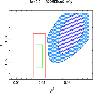
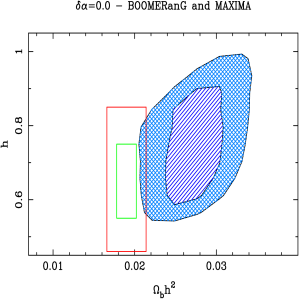
FIG. 2.: The marginalized likelihoods in the $\Omega_{\rm b}h^{2}$—$h$ plane for the B98 (left) and B98+M99 (right) data. Shown are the 1-$\sigma$ (68% confidence) and 2-$\sigma$ (95%) contours, plus a box showing the region $h=0.65\pm 0.1$ and $\Omega_{\rm b}h^{2}=0.019\pm 0.0012$ and the corresponding 2-$\sigma$ contour. Note that the regions corresponding to the direct and CMB measurements do not overlap when one includes only B98 and there is only very little overlap when M99 is included as well.

To illustrate this point we have computed flat band power estimates for the CMB anisotropies in the range probed by the B98 and M99 experiments for flat $\Lambda$CDM models for a grid of cosmological parameters ($h=0.45-1.05$, $\Delta h=0.05$; $\Omega_{\rm b}h^{2}=0.007-0.040$, $\Delta\Omega_{\rm b}h^{2}=0.003;$ $\Omega_{\rm m}=0.2-0.8$, $\Delta\Omega_{\rm m}=0.1;$ $n_{\rm S}=0.8-1.1$, $\Delta n_{\rm S}=0.05$.), computed the likelihood of the models given the data and then marginalized over the parameters $n_{\rm S}$ and $\Omega_{m}$, assuming that (1) $A_{\rm S}$ be that measured by COBE with Gaussian errors of approximately 15% [31], (2) the B98 calibration errors are Gaussian, with an amplitude of $20\%$, and (3) the M99 calibration errors have an equivalent amplitude of $8\%$ with Gaussian correlations with respect to the other measurements when included. The relative likelihood contours are presented in Fig. 2 for B98 alone and for it combined with M99, included also is a box giving an idea of where the direct limits lie. It is clear that the CMB measurements disagree with the direct measures of these cosmological parameters at the $2\sigma$ level if one only takes into account B98, and this conclusion is only slightly weakened by the inclusion of M99. Thus, the CMB measurements appear to be in conflict with the baryon density inferred from nucleosynthesis and either the measurements of $h$ or the theoretical prejudice of $\Omega_{\rm tot}=1$. (This is supported by the analyses of refs. [3, 7].)

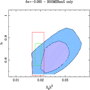
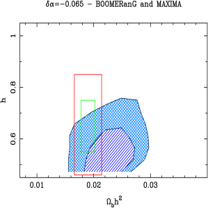
FIG. 3.: The equivalent to Fig. 2, but with $\delta\alpha=-0.065$. Notice that now the 1- and 2-$\sigma$ contours are now in good agreement with the region preferred by direct measurements which have been assumed to be unaffected by the change in $\alpha$.

These conflicts can be resolved if one considers changing the value of $\alpha$ at last scattering. If we repeat the above analysis, there is a marked improvement in the consistency of the CMB measurements with the direct measurements of $h$ and $\Omega_{\rm b}h^{2}$ when $\delta\alpha<0$. We illustrate this point in Fig. 3 where $\alpha$ is reduced by 6.5% from its present day value, that is $\delta\alpha=-0.065$. This shift brings the CMB into better agreement with the direct measurements. It should be noted, however, that the direct measurements themselves may also be modified by a change in the fine structure constant, which we have not attempted to model here. This issue we will discuss further in section IV.

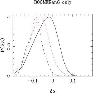
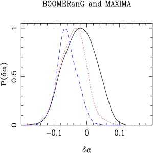
FIG. 4.: The likelihood marginalized over the cosmological parameters $h$, $\Omega_{\rm m}$, $\Omega_{\rm b}h^{2}$, $n_{\rm S}$ and $A_{\rm S}$ as a function of $\delta\alpha$ with no prior (P0 - solid line), the age prior (P1 - dotted line) and the combined $h$/strong BBN prior (P4 - dashed line). All the probability distributions are biased toward $\delta\alpha<0$, with those for P4 implying a substantial probability that $\delta\alpha<0$.

	Boomerang Only				Boomerang & Maxima
Prior	$\delta\alpha$ (%)	$68.5\%$ CL	$95.5\%$ CL	${\cal{P}}(\delta\alpha<0)$	$\delta\alpha$ (%)	$68.5\%$ CL	$95.5\%$ CL	${\cal{P}}(\delta\alpha<0)$
P0	-2.0	${}^{+4.5}_{-5.0}$	${}^{+8.0}_{-13}$	$72\%$	-2.0	${}^{+4.5}_{-5.0}$	${}^{+8.0}_{-9.0}$	$63\%$
P1	-6.0	${}^{+4.0}_{-5.0}$	${}^{+8.5}_{-11}$	$91\%$	-3.0	${}^{+3.0}_{-5.0}$	${}^{+7.0}_{-8.0}$	$84\%$
P2	-5.0	${}^{+4.0}_{-4.0}$	${}^{+7.5}_{-9.0}$	$89\%$	-2.5	${}^{+2.5}_{-4.0}$	${}^{+6.0}_{-7.0}$	$77\%$
P3	-6.5	${}^{+4.0}_{-4.0}$	${}^{+8.0}_{-8.5}$	$94\%$	-3.5	${}^{+3.5}_{-3.5}$	${}^{+6.0}_{-6.5}$	$84\%$
P4	-8.5	${}^{+3.0}_{-4.0}$	${}^{+7.0}_{-8.0}$	$99\%$	-6.5	${}^{+3.5}_{-2.5}$	${}^{+6.5}_{-5.0}$	$97\%$
P5	-7.0	${}^{+3.0}_{-2.5}$	${}^{+6.0}_{-8.0}$	$98\%$	-5.5	${}^{+3.0}_{-2.5}$	${}^{+5.5}_{-7.0}$	$96\%$

TABLE I.: The peaks of the probability distribution functions for $\delta\alpha$ for the various priors for the B98 data alone and for the combined data sets. Also tabulated are the 1- and 2-$\sigma$ intervals and the integrated probability that $\delta\alpha<0.$ Note that all the probability distributions favor $\delta\alpha<0$.

To further quantify this, one can derive likelihoods for the value of $\delta\alpha$ by marginalizing over all the other cosmological parameters, including the Hubble constant and baryon density. We have done this for a wide range of $\delta\alpha$ using a slightly wider spacing than above — $\Delta h=0.1$ and $\Delta\Omega_{\rm b}h^{2}=0.006$. In addition to the CMB data, we consider a number of possible prior assumptions for the parameters, particularly focusing on those involving $h$ and $\Omega_{\rm b}h^{2}$. Results based on the CMB data alone, without any prior, are labelled P0. We have included two simple priors incorporating fairly weak constraints on the age of the universe (P1: $t_{0}>11.5$ Gyr) or on the Hubble constant (P2: $h=0.65\pm 0.1$.) These tend to have similar effects, as both effectively cut off the large $h$ region of parameter space. We have also considered adding weak and strong priors on the baryon density to the previously assumed Hubble constant prior, (P3: P2 + $\Omega_{\rm b}h^{2}=0.019\pm 0.006$) and (P4: P2 + $\Omega_{\rm b}h^{2}=0.019\pm 0.0012$.) Finally, we combine the age, Hubble constant, and strong baryon density priors with a constraint based on the cluster baryon fraction (P5: P1 + P4 + $f_{\rm b}=0.067\pm 0.008$.), where $f_{\rm b}$ is the fraction of baryons to total mass deduced from X-ray observations of rich clusters. In each case the quoted error bars above are taken to be the $68\%$ (1-$\sigma$) confidence level.

The result of these marginalized distributions for $\delta\alpha$ for P0, P1 and P4 are shown in Fig. 4, and the basic properties of these distributions are displayed in Table I for all the priors. As can be seen, in the absence of any priors the data prefer a value for $\alpha$ at last scattering a few percent lower than its present value, but the constraint is fairly weak. Considering only the B99 data and adding fairly weak constraints on the age or $h$ gives a significantly stronger signal, suggesting a detection of variation in $\alpha$ at the 1-$\sigma$ level. Finally, if one includes the stronger constraints that the baryon density is low, then the evidence for variation in $\alpha$ is significant at the 2-$\sigma$ level. Including the M99 data weakens these detections somewhat, but not dramatically.

One can understand the effects of the priors in light of our earlier discussion of how the CMB anisotropies depend on $\delta\alpha$. By allowing $h$ and $\Omega_{\rm b}h^{2}$ to vary freely one can fit both the primary peak position and secondary peak heights either with $\delta\alpha=0$ or $\delta\alpha\neq 0$, and as we have already seen in Fig. 2, fixing $\delta\alpha=0$ requires large values of $h$ and $\Omega_{\rm b}h^{2}$. The constraint on $h$ comes primarily from the position of the primary peak. When one allows the time of recombination to change due to a variation in $\delta\alpha$, the high value of $h$ can be offset by an increase in $c_{\rm s}\eta_{*}$, making models with a lower values of $h$ and $\delta\alpha<0$ equally likely. If one further assumes a prior such as P1 or P2 which penalizes high $h$, the models with $\delta\alpha<0$ become favored over those with $\delta\alpha=0$. A similar line of argument can be applied to $\Omega_{\rm b}h^{2}$. When $\delta\alpha=0$ a high value of $\Omega_{\rm b}h^{2}(\approx 0.031)$ is favored, but when one allows $\delta\alpha$ to vary, the approximate degeneracy between $\delta\alpha$ and $\Omega_{\rm b}h^{2}$ makes models with a lower value of $\Omega_{\rm b}h^{2}$ and $\delta\alpha<0$ equally likely. Clearly, the inclusion of a constraint which penalizes high $\Omega_{\rm b}h^{2}$ will favor models with $\delta\alpha<0$. The remarkable aspect of this is that the inclusion of a single parameter, $\delta\alpha$, has the effect of improving the fit to the observations through two physically very distinct mechanisms.

The conclusions are substantiated by examining the best fit models listed in Tables II and III, and plotted compared to the B98 data in Fig.5 and to the combined dataset in Fig. 6. Except for P0 in the case of B98 alone, and P0 and P1 in the case of B98 and M99, the reduced $\chi^{2}$ of the best fits are decreased by allowing $\alpha$ to vary, but the fits are only significantly improved when one assumes a strong prior for the baryon density (P3-P5). When considering just the B98 data, the $\chi^{2}$ appears to be somewhat smaller than the number of degrees of freedom, so that the reduced $\chi^{2}$ are significantly less than one, which in turn suggests that the error bars of the B98 data may be overestimated. The reduced $\chi^{2}$ no longer appear low when the M99 data are included in the analysis.

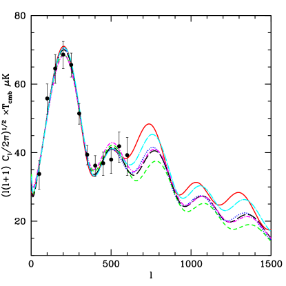
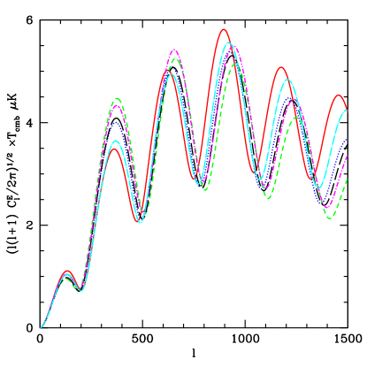
FIG. 5.: The angular power spectra of temperature anisotropies and polarization for the best fit models to the B98 data from Table II. Included are P0 with $\delta\alpha=0$ (Long dashed-dot line) and P1 (Solid), P2 (dotted), P3/P4 (short dashed) P5 (short-dash dotted) all with $\delta\alpha\neq 0$, along with the B98 data. The best fit normalization changes for different models, therefore each curve has been appropriately normalized so that they can all be plotted with the data on the same graph.

Prior	$\delta\alpha$	$h$	$\Omega_{\rm b}h^{2}$	$\Omega_{\rm m}$	$n_{\rm S}$	$R_{\rm B98}$	$\chi^{2}$
P0	0.0	0.95	0.031	0.2	0.925	1.00	4.03
	-0.020	0.85	0.031	0.3	0.975	0.92	3.90
P1	0.0	0.85	0.025	0.2	0.850	1.12	5.09
	-0.055	0.75	0.025	0.2	0.900	0.92	4.00
P2	0.0	0.75	0.031	0.6	0.975	1.00	5.66
	-0.070	0.65	0.025	0.3	0.900	0.94	4.10
P3	0.0	0.65	0.025	0.6	0.900	1.14	7.84
	-0.080	0.65	0.019	0.2	0.850	0.98	4.29
P4	0.0	0.75	0.019	0.2	0.800	1.16	10.15
	-0.080	0.65	0.019	0.2	0.850	0.98	4.29
P5	0.0	0.65	0.019	0.4	0.800	1.32	12.13
	-0.070	0.55	0.019	0.4	0.850	1.08	6.60

TABLE II.: The best fit models for the B98 data only with the various priors, with and without allowing variations in $\alpha$. The number of degrees of freedom (number of data points minus number of theoretical parameters) for the fits are roughly between 7 and 10 when $\delta\alpha=0$, depending on the number of constraints. (This is reduced by 1 for the $\delta\alpha\neq 0$ models.) Models with stronger priors included in the likelihood effectively have more data and thus more degrees of freedom. Note that the fits are substantially improved by allowing $\delta\alpha\neq 0$ when there is a prior assumption on $\Omega_{\rm b}h^{2}$ and that the reduced $\chi^{2}$ are generally less than one. $R_{\rm B98}$ is the ratio of the COBE and B98 normalizations for the $C_{\ell}$’s.

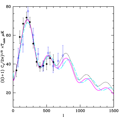
FIG. 6.: The angular power spectra of temperature anisotropies for the best fit models to the B98 and M99 data from Table III. Included are P0 with $\delta\alpha=0$ (dotted line) and P4 with $\delta\alpha=0$ (dashed line) with $\delta\alpha\neq 0$ (solid line). With the strong BBN constraint on the baryon density, the $\delta\alpha\neq 0$ case provides a much better fit than the $\delta\alpha=0$ case. As for Fig. 5 we have normalized so that all the models can be presented on the same plot. In doing this we have fixed the calibration of the B98 data relative to the M99 calibration to be 15% higher than its nominal value.

Prior	$\delta\alpha$	$h$	$\Omega_{\rm b}h^{2}$	$\Omega_{\rm m}$	$n_{\rm S}$	$R_{\rm B98}$	$R_{\rm M99}$	$\chi^{2}$
P0	0.0	0.75	0.025	0.3	0.925	0.92	1.06	16.43
	-0.025	0.65	0.025	0.4	0.925	0.92	1.06	15.82
P1	0.0	0.75	0.025	0.3	0.925	0.92	1.06	16.43
	-0.025	0.65	0.025	0.4	0.925	0.92	1.06	15.82
P2	0.0	0.65	0.025	0.5	0.925	0.98	1.09	17.13
	-0.025	0.65	0.025	0.4	0.925	0.92	1.06	15.82
P3	0.0	0.65	0.025	0.5	0.925	0.98	1.09	18.13
	-0.025	0.65	0.025	0.4	0.925	0.92	1.06	16.82
P4	0.0	0.75	0.019	0.2	0.850	1.00	1.15	21.89
	-0.065	0.65	0.019	0.2	0.900	0.82	0.97	18.08
P5	0.0	0.65	0.019	0.3	0.850	1.00	1.15	24.43
	-0.055	0.55	0.019	0.4	0.900	0.90	1.03	18.96

TABLE III.: The best fit models for the B98 and M89 data with the various priors, with $\delta\alpha=0$ and $\delta\alpha\neq 0$. The number of degrees of freedom for the fits are in the range 16-19 for $\delta\alpha=0$. (Again, it is reduced by 1 when $\delta\alpha\neq 0$). $R_{\rm M99}$ is the ratio of the COBE and M99 normalizations for the $C_{\ell}$s.

IV Discussion

In the previous section we presented evidence for a variation in $\alpha$ using recent CMB observations. If confirmed by subsequent observations this would be a truly remarkable result. In this section we will discuss the various aspects of our analysis, focusing on the potential uncertainties.

First, we should make some comments on the details of our statistical procedure and the models which we have probed. We make the approximation that the CMB data points are statistically independent and Gaussianly distributed, with window functions given by flat band powers in $\ell$. This is also an assumption in the analysis of ref. [7], but not in those of the BOOMERanG and MAXIMA collaborations [8, 9] where the exact experimental window functions were used. Since the analysis presented here for $\delta\alpha=0$ agrees qualitatively with those other analyses, we believe these approximations should be sufficient for our purposes. The B98 data has more points (12 versus 10) and smaller errors than the M99 data, and generally provides stronger constraints. While both data sets suggest the secondary peak is suppressed relative to the first Doppler peak, the M99 data shows no evidence for a left-ward shift of the peak. Thus, including it tends to weaken the evidence for a time varying $\alpha.$

We include in our calculations the uncertainties in the absolute calibrations of the data sets, which is necessary in order for them to be consistent with each other. The B98 data was normalized by the CMB dipole, which is subject to large systematic errors, and their quoted calibration error is 20% in the power. The M99 experiment was also able calibrate off of Jupiter, and has only an 8% error. Best fit models allowing both of these to vary seem to prefer an increase of roughly 15% in the relative B98/M99 power calibration (see, for example, Table III).

We should also note that the range of models we use in our analysis does not include many cosmological scenarios that are often considered. We have excluded the possibility of tensor fluctuations with a spectral index $n_{\rm T}$ and amplitude $A_{\rm T}$, a hot dark matter component $\Omega_{\nu}$, and also that of early reionization often quantified by $\tau_{\rm R}$, the optical depth to reionization. These were included in ref.[7] and were found to have little or no bearing on the preferred values of $\Omega_{\rm b}h^{2}$ and $h$ since these parameters are effectively orthogonal given the present data. In fact, in ref. [8] it was suggested that there is a degeneracy between $n_{\rm S}$ and $\tau_{\rm R}$ for the angular scales probed in B98; our unusually low values of $n_{\rm S}$, therefore, take into account the possibility of reionization at moderate redshift with $n_{\rm S}=1$ being compatible with the data.

We have investigated this by constructing the Fisher matrix which quantifies the effects of changing parameters has on the measured band powers ${\cal B}_{i}$,

$${\cal{F}}_{ab}={\partial{\cal B}_{i}\over\partial p_{a}}C^{-1}_{ij}{\partial{\cal B}_{j}\over\partial p_{b}},$$ (5)

where $p_{a}$ are the parameters ($\Omega_{\rm m}h^{2},\Omega_{\rm b}h^{2},h,\delta\alpha,n_{\rm S},\tau_{\rm R},A_{S}$) and $C_{ij}$ is the data covariance matrix, assumed diagonal except for the calibration uncertainties. We find the strongest degeneracy of $\delta\alpha$ to be with $\Omega_{\rm m}h^{2}$, but there are also significant overlaps with $h$ and $\Omega_{\rm b}h^{2}$; all of which are consistent with the simple theoretical arguments in Section II. Our inferred errors on $\delta\alpha$ from Figure 4 are quite consistent with those expected by computing inverse Fisher matrix for the best fit model with P0. The matrix is also largely block diagonal as one might have expected, with $n_{\rm S},\tau_{\rm R},A_{S}$ being largely orthogonal to the other variables, but with significant overlap amongst themselves, confirming that $n_{\rm S}$ and $\tau_{\rm R}$ are degenerate given the present data.

Knowledge of the Fisher matrix allows us to investigate the impact future CMB measurements might have on further constraining parameters. If the error bars of the B98 and M99 experiments are reduced by a factor of two, the errors on $\alpha$ (and indeed on most parameters) are reduced by a comparable factor. Hence, improved sensitivity with the same angular coverage is an important goal. We have also considered the impact of a hypothetical measurement of the third peak, centered at $\ell=800$, as well as a detection of the first polarization peak centered at $\ell=350$, assuming 10% errors on a flat band power measurement in each case. Both, particularly the polarization measurement, help to reduce uncertainties in $\Omega_{\rm m}h^{2}$ and $\Omega_{\rm b}h^{2}$, but disappointingly neither do very well in reducing the uncertainties in $\delta\alpha$. It should be noted that a weakness of this band power based approach is that the conclusions will depend somewhat on how the data are binned, particularly if the models vary greatly across the bins.

Having argued that our statistical procedure and the models which we have probed provide a robust detection of a variation in $\alpha$ given prior assumptions from direct measurements of $h$ and $\Omega_{\rm b}h^{2}$ in a flat universe, we now turn to the more difficult issue of the effect of such a variation on these direct measurements. This pertains primarily to those associated with BBN since the measurements of $h$, $t_{0}$ and $f_{b}$ are made at very low redshifts and therefore will be relatively insensitive to these changes.

Since electromagnetic effects are ubiquitous in BBN, it is clear that there must exist a constraint on $\delta\alpha(t_{\rm nuc})$ from the consistency of BBN with light element abundances. There are two approaches to this problem documented in the literature. The first [23, 24] is to use only the observations of ${}^{4}{\rm He}$, which are thought to be the most reliable. One can make a very simple estimate of the primordial ${}^{4}{\rm He}$ abundance, in terms of $m_{n}/m_{p}$, the neutron to proton mass ratio. However, expressing this in terms of $\alpha$ cannot be done in a model independent way because it involves a subtle interplay between electromagnetic, weak and strong interaction effects which have not been understood completely within QCD. Therefore, tight limits on $\delta\alpha(t_{\rm nuc})$ computed in this way should be treated with some caution.

A more reliable alternative [25] is to make a detailed analysis of how changes in $\alpha$ can effect all the light abundances and derive a constraint from demanding consistency with their observed values. Although this involves a number of complicated nuclear reaction rates, it turns out that a model independent constraint might be possible at the level of around a few percent. In fact, it was suggested in ref. [25] that $|\delta\alpha(t_{\rm nuc})|\approx 0.02$ could help BBN fit the observed light element abundances better. However, even this value should be treated with some caution since there are further uncertainties which might could modify it by as much as a factor of two [35].

Furthermore, the implied value of $\Omega_{\rm b}h^{2}$ is likely to change as a function of $\delta\alpha(t_{\rm nuc})$. For example, one might expect that [35]

$$\Omega_{\rm b}h^{2}\left[\delta\alpha(t_{\rm nuc})\right]=\left[1+A\delta\alpha(t_{\rm nuc})\right]\Omega_{\rm b}h^{2}\left[0\right]$$ (6)

for small values of $\delta\alpha(t_{\rm nuc})$ where the coefficient is expected to be of order $A\sim{\cal O}(1)$. The amplitude and sign of the proportionality constant $A$ will clearly have some influence on our conclusions. In particular, if decreasing $\alpha$ increases the inferred baryon density $(A<0)$, then it may be possible to fit the data with a smaller change in $\alpha$. However, if the opposite is true $(A>0)$, then it may prove a better fit if the fine structure constant is larger at last scattering, contrary to our present results.

To make contact with the earlier discussion, one needs to relate $\delta\alpha(t_{\rm nuc})$ and $\delta\alpha(t_{\rm rec})$ which requires a model for how the variation in $\alpha$ is realized. If $\alpha$ is increasing with time as we have suggested here, then it might be sensible to assume that it has done so monotonically and, therefore, $\delta\alpha(t_{\rm nuc})<\delta\alpha(t_{\rm rec})$. Given the uncertainties, the constraint from BBN on $\delta\alpha(t_{\rm nuc})$ would appear to be consistent with this relation given the fairly small values of $\delta\alpha(t_{\rm rec})$ required for a good fit to the CMB data. However, this certainly motivates a critical appraisal of the exact constraint on $\delta\alpha$ from BBN. Including the effect of changing $\alpha$ on the BBN measurements would require knowledge of the parameter $A$ and we have not attempted to incorporate this into our analysis. This issue should be revisited in future work when the $\alpha$ dependence of the BBN constraints are better understood.

Finally, we should mention that realistic models in which $\alpha$ varies may contain one or more light scalar fields which mediate the precise variation. Clearly, if such a field exists it should be included in the calculation of the CMB anisotropies in the Boltzmann hierarchy of CMBFAST, either explicitly or as a extra relativistic degree of freedom. This would allow a subsequent analysis to include effects of the time variation of $\alpha$, rather than just a change between the time of recombination and the present day. Such a field could have significant energy density during the epochs important for structure formation (after the time of radiation-matter equality) and it may even be possible for such a field to act as a quintessence field [37], removing the need for $\Lambda$.

V Conclusions

The most recent CMB data provide strong evidence yet that the universe is, at least approximately, spatially flat. The B98 data, however, is not entirely consistent with spatial flatness and direct measurements of other cosmological parameters. The situation is only slightly improved when the M99 data is included. However, if the fine structure constant was a few percent smaller when the photons were last scattered, then a model can be found which is consistent with all observations. It is clear that a change in the $\alpha$ is not the only possible explanation for such observations, and the evidence we present here could equally well be thought of as favoring other delayed recombination models, for example, that presented in ref. [12].

The evidence for a time variation in the fine structure constant is significant when a tight prior is assumed for the baryon density. However, the baryon density inferred from measurements of primordial abundances depends on nuclear physics processes at times long before last scattering at the epoch of BBN. We have argued that the values of $\delta\alpha(t_{\rm rec})\sim-0.05$ that we have deduced are consistent with BBN given the uncertainties assuming that the variation in $\alpha$ is monotonic, but that inclusion of the effect of varying $\alpha$ on the inferred value of $\Omega_{\rm b}h^{2}$ for a given Deuterium abundance has been ignored, mainly due to lack of quantitative information.

Stronger conclusions must, of course, wait for better data, such as might come from the satellite experiments MAP and PLANCK. In particular, these will be able to confirm whether the inconsistencies of flat models with direct measurements and the CMB data (such as a slight shift of features to larger scales) are real. In addition, these experiments should be able to break the degeneracy between a changing $\alpha$ and $\Omega_{\rm b}h^{2}$, so that a change in $\alpha$ can be tested independently of what occurred at nucleosynthesis. It is clear from Fig. 5 that the best fit models can differ greatly for $\ell>600$ in temperature anisotropies and the polarization; any experiment which probes the CMB in these areas will be useful in breaking these degeneracies, although the results of our Fisher matrix analysis suggest they will require considerable sensitivity.

Having presented our case for a few percent variation in $\alpha$ at around $z\approx 1000$, it is interesting to compare to the other claimed detection of a change in $\alpha$ around $z\approx 1$, and speculate as to an explanation. Naively, $\delta\alpha(z\approx 1000)\sim-0.01$ and $\delta\alpha(z\approx 1)\sim-10^{-5}$ might suggest that $\delta\alpha\propto z$, but this would be incompatible with BBN if extrapolated back to $z\approx 10^{9}-10^{10}$. In order to have a chance of being consistent with BBN, such a scenario would require that the variation in $\alpha$ terminated at some point shortly before recombination, that is, $\delta\alpha(t_{\rm nuc})\sim\delta\alpha(t_{\rm rec})$. At first sight coupling $\alpha$ non-minimally to gravity via the Ricci scalar or the trace of the energy-momentum tensor as suggested in ref. [18], both of which are zero in the radiation-era and non-zero in the matter-era, might seem an attractive solution since the variation in $\alpha$ would begin at the onset of matter domination. Clearly, such ideas could have a profound impact on understanding of Grand Unification and this particular interpretation of the most recent observations presented here opens up a wide range of interesting possibilities for future research in this area.

- [1] P. Steinhardt and J.P. Ostriker, Nature (London) 377, 600 (1995). N. Bahcall, J.P. Ostriker, S. Perlmutter and P. Steinhardt, Science 284, 1481 (1999).
- [2] G. Jungmann et al, Phys. Rev. Lett. 76, 1007 (1996). G. Jungmann et al, Phys. Rev. D54, 1332 (1996).
- [3] P. de Bernardis et al, Nature (London) 404, 955 (2000).
- [4] S. Hanany et al, astro-ph/0005123.
- [5] W. Hu, Nature (London) 404, 939 (2000).
- [6] M. White, D. Scott and E. Pierpaoli, astro-ph/0004385.
- [7] M. Tegmark and M. Zaldariagga, astro-ph/0004393.
- [8] A. Lange et al, astro-ph/0005004.
- [9] A. Balbi et al, astro-ph/0005124.
- [10] C. Copi, D.N. Schramm and M.S. Turner, Science 267, 192 (1995).
- [11] S. Burles and D. Tytler, Astrophys. J. 507, 732 (1998).
- [12] P.J.E. Peebles, S. Seager and W. Hu, astro-ph/0004389.
- [13] D.W. Sciama and A.L. Melott, Phys. Rev. D25, 2214 (1982).
- [14] P.Salati and J.C. Wallet, Phys. Lett. B 144, 61 (1984).
- [15] J. Weller, R.A. Battye and A. Albrecht, Phys. Rev. D60, 103520 (1999).
- [16] S. Hannestad, Phys. Rev. D60, 023515 (1999).
- [17] M. Kaplinhhat, R.J. Scherrer and M.S. Turner, Phys. Rev.. D60123508
- [18] J.D. Bekenstein, Comments on Astro. 8, 89 (1979).
- [19] J.D. Barrow and J. Magueijo, Phys. Lett. 443B, 104 (1999).
- [20] A. Albrecht and J. Magueijo, Phys. Rev. 59, 043516 (1999).
- [21] J.D. Barrow and A. Albrecht, Astrophys. J. 532, L87 (2000).
- [22] A.I. Shylakhter, Nature (London 264, 340 (1976). T. Damour and F. Dyson, Nucl. Phys. B480, 37 (1996).
- [23] E.W. Kolb, M.J. Perry and T.P. Walker, Phys. Rev. D33, 869 (1986).
- [24] J.D. Barrow, Phys. Rev. D35, 1805 (1987).
- [25] L. Bergstrom, S. Iguri and H. Rubinstein, Phys. Rev. D60, 045005 (1999).
- [26] L.L. Cowie and A. Songalia, Astrophys. J. 453, 596 (1995). M.J. Drinkwater et al, Mon. Not. Roy. Astro. Soc. 295, 457 (1998).
- [27] J.K. Webb et al, Phys. Rev. Lett. 82, 884 (1999).
- [28] U. Seljak and M. Zaldariagga, Astrophys. J. 437, 469 (1996).
- [29] P.J.E. Peebles, Astrophys. J. 153, 1 (1968).
- [30] R.J. Gould and R.K. Thakur, Ann. Phys. (N.Y.) 61, 1 (1970).
- [31] C. Bennett, et al., Astrophys. J. 464, L1 (1996). E. Bunn and M. White, Astrophys. J. 450, 477 (1995).
- [32] W. Hu, D. Scott, N. Sugiyama and M. White, Phys. Rev. D52, 5498 (1995).
- [33] W. Hu and N. Sugiyama, Astrophys. J. 471, 542 (1996).
- [34] J. Silk, Astrophys. J. 151, 459 (1968).
- [35] R. Lopez, Private communication.
- [36] W. Marciano, Phys. Rev. Lett. 52, 489 (1984).
- [37] R. Bean and J. Magueijo, astro-ph/0007199.