Analysis of cosmic microwave background data on an incomplete sky

Abstract

Measurement of the angular power spectrum of the cosmic microwave background is most often based on a spherical harmonic analysis of the observed temperature anisotropies. Even if all-sky maps are obtained, however, it is likely that the region around the Galactic plane will have to be removed due to its strong microwave emissions. The spherical harmonics are not orthogonal on the cut sky, but an orthonormal basis set can be constructed from a linear combination of the original functions. Previous implementations of this technique, based on Gram-Schmidt orthogonalisation, were limited to maximum Legendre multipoles of $l_{\mathrm{m}ax}\la 50$ as they required all the modes have appreciable support on the cut sky, whereas for large $l_{\mathrm{m}ax}$ the fraction of modes supported is equal to the fractional area of the region retained. This problem is solved by using a singular value decomposition to remove the poorly-supported basis functions, although the treatment of the non-cosmological monopole and dipole modes necessarily becomes more complicated. A further difficulty is posed by computational limitations – orthogonalisation for a general cut requires $O(l_{\mathrm{m}ax}^{6})$ operations and $O(l_{\mathrm{m}ax}^{4})$ storage and so is impractical for $l_{\mathrm{m}ax}\ga 200$ at present. These problems are circumvented for the special case of constant (Galactic) latitude cuts, for which the storage requirements scale as $O(l_{\mathrm{m}ax}^{2})$ and the operations count scales as $O(l_{\mathrm{m}ax}^{4})$. Less clear, however, is the stage of the data analysis at which the cut is best applied. As convolution is ill-defined on the incomplete sphere, beam-deconvolution should not be performed after the cut, and, if all-sky component separation is as successful as simulations indicate, the Galactic plane should probably be removed immediately prior to power spectrum estimation.

1 Introduction

Since the first measurements of the temperature anisotropy of the cosmic microwave background (CMB) by the Cosmic Background Explorer (COBE) satellite (Smoot et al. 1992), a number of sophisticated experiments have been undertaken to measure the fluctuations at higher resolutions and sensitivities (e.g. Scott et al. 1996; Tanaka et al. 1996; Netterfield et al. 1997; de Oliveira-Costa et al. 1998; Coble et al. 1999; de Bernardis et al. 2000; Wilson et al. 2000; Padin et al. 2001; Halverson et al. 2001; Lee et al. 2001; Netterfield et al. 2001). The primary result of these experiments has been the measurement of the angular power spectrum of the CMB to Legendre multipoles of up to $l\simeq 1000$, which places strong constraints on a number of cosmological parameters (Lineweaver 1998; Efstathiou et al. 1999; de Bernardis et al. 2000; Netterfield et al. 2001; Wang, Tegmark & Zaldarriaga 2001 and references therein). In the future the Microwave Anisotropy Probe (MAP; e.g. Jarosik et al. 1998) and the Planck satellite (e.g. Bersanelli et al. 1996) will produce maps of the microwave sky with resolutions of between 5 and 30 arcmin at a number of frequencies. Such extraordinary data-sets, consisting of millions of independent measurements, will clearly require novel analysis techniques.

One of the many difficulties is the treatment of the non-cosmological contributions to the observed microwave sky. Dust, synchrotron and free-free emission from the Galaxy (e.g. Haslam et al. 1982; Schlegel, Finkbinder & Davies 1998); radio galaxies and other extra-Galactic ‘point’ sources (e.g. Toffolatti et al. 1998); and the Sunyaev-Zel’dovich (1970) effect caused by galaxy clusters (e.g. Birkinshaw 1999) all obscure the CMB at some level (see Hu, Sugiyama & Silk 1997 or Barreiro 2000 for more complete reviews), although these components have quite distinct spectral properties and so can be separated using multi-frequency observations (e.g. Bennett et al. 1992; Tegmark & Efstathiou 1996; Hobson et al. 1998; Bouchet & Gispert 1999; Jones, Hobson & Lasenby 1999; Baccigalupi et al. 2000). However these techniques are not likely to be able to extract the Galactic emissions completely (Stolyarov et al. 2001), leaving the removal of the Galactic plane as the only option. The Galaxy contributes relatively little at high latitudes (e.g. Haslam et al. 1982; Schlegel et al. 1998) so this is an acceptable, if not optimal, solution. For instance, Górski et al. (1994) removed the band within 20 deg of the Galactic plane to estimate the power spectrum of the two-year COBE Differential Microwave Radiometer sky maps, and similar cuts have been proposed by both the MAP and Planck collaborations. An essentially equivalent problem is posed if the survey’s sky coverage is incomplete, although there is less choice about the geometry of the cut in this case.

A number of aspects of the analysis become more difficult on an incomplete sphere, one of the most obvious reasons being that the spherical harmonics are no longer an orthonormal basis set. The most successful component separation techniques to date (e.g. Hobson et al. 1998; Bouchet & Gispert 1999) rely on a mode-by-mode analysis which explicitly utilises the orthogonality of the spherical harmonics, although it may be preferable to remove the Galactic plane only when estimating the CMB power spectrum. Unbiased power spectrum estimation using the spherical harmonics is possible on the cut sky (Wandelt, Górski & Hivon 2001), but the covariance structure of the resulting psuedo-harmonics is far from ideal, so analysis using an orthonormal basis set is preferable. In particular the noise covariance matrix remains diagonal in the case of spatially uniform (and uncorrelated) noise.

It is possible to construct an orthonormal basis set from linear combinations of the spherical harmonics, and an elegant implementation of this, based on Cholesky decomposition of the coupling matrix of the spherical harmonics on the cut sky, was described by Górski (1994). However the coupling matrix becomes ill-conditioned for $l_{\mathrm{m}ax}\ga 50$, and so this method cannot be used to perform cut-sky orthogonalisation for either the MAP experiment (with $l_{\mathrm{m}ax}\simeq 1500$) or the Planck mission (with $l_{\mathrm{m}ax}\simeq 2500$).

A general formalism for orthogonalisation of the spherical harmonics is presented in Section 2, although implementation to high $l_{\mathrm{m}ax}$ is only possible at present in the special case of a constant latitude cut. The relationship between the various harmonic coefficients is discussed in Section 3, and the extension of these results to CMB analysis techniques (specifically component separation and power spectrum estimation) is covered in Section 4. The results are summarised and future possibilities are discussed in Section 5. Finally, the chosen conventions for the spherical harmonics are defined in Appendix A; formulæ for integrals of the products of Legendre functions are given in Appendix B; and the treatment of the non-cosmological monopole and dipole modes are discussed in Appendix C.

2 Orthogonalisation of scalar basis
functions

The physics of the CMB is most naturally expressed in Fourier space, and it is standard practice to represent sky maps by their harmonic coefficients. The basis functions chosen here are the real spherical harmonics, $Y_{l,m}(\hat{\mbox{\boldmath${r}$}})$ (as defined in Appendix A), which form an orthonormal basis on the complete sphere, $S$. In general $l\geq 0$ and $-l\leq m\leq l$, although in practice a finite $l_{\mathrm{m}ax}$ must be used, which implies a band-limit. It is convenient to combine the two indices, allowing the basis set to be expressed as a vector, $\mbox{\boldmath${Y}$}(\hat{\mbox{\boldmath${r}$}})=[Y_{1}(\hat{\mbox{\boldmath${r}$}}),Y_{2}(\hat{\mbox{\boldmath${r}$}}),\ldots,Y_{i_{\mathrm{m}ax}}(\hat{\mbox{\boldmath${r}$}})]^{\mathrm{T}}$, where $i_{\mathrm{m}ax}=(l_{\mathrm{m}ax}+1)^{2}$. There are several reasonable choices for the indexing, $i(l,m)$, most notably grouping coefficients in $l$ or $m$, as defined in Appendix A. Grouping in $l$ is most natural for power spectrum estimation, but grouping in $m$ is more efficient computationally in cases of azimuthal symmetry (Section 2.3).

The spherical harmonics are not orthogonal on the incomplete sphere ${S^{\prime}}$, as can be seen from the structure of their coupling matrix (Section 2.1). A decomposition of the coupling matrix can be used to construct an orthonormal basis set (Section 2.2), but implementation to high-resolution is currently possible only in the special case of constant latitude cuts (Section 2.3).

2.1 The coupling matrix

The coupling matrix of a set of functions encodes their orthogonality and normalisation properties over a given range. In the case of the spherical harmonics on the incomplete sphere it is given by

$$\mbox{\bf\sf{C}}=\int_{{S^{\prime}}}\mbox{\boldmath${Y}$}(\hat{\mbox{\boldmath${r}$}})\mbox{\boldmath${Y}$}^{\mathrm{T}}(\hat{\mbox{\boldmath${r}$}})\,{\mathrm{d}\Omega}.$$ (1)

If ${S^{\prime}}=S$ then the harmonics are orthonormal and $\mbox{\bf\sf{C}}=\mbox{\bf\sf{I}}$; otherwise the off-diagonal elements are non-zero, indicating that the basis functions are non-orthogonal.

An alternative formulation is to introduce a window function, $w(\hat{\mbox{\boldmath${r}$}})$, so that

$$\mbox{\bf\sf{C}}=\int_{S}w^{2}(\hat{\mbox{\boldmath${r}$}})\mbox{\boldmath${Y}$}(\hat{\mbox{\boldmath${r}$}})\mbox{\boldmath${Y}$}^{\mathrm{T}}(\hat{\mbox{\boldmath${r}$}})\,{\mathrm{d}\Omega}.$$ (2)

In some ways this approach is more flexible, as $w(\hat{\mbox{\boldmath${r}$}})$ can either be a smoothly-varying apodizing function (cf. Tegmark 1997) or take the form

$$w_{{S^{\prime}}}(\hat{\mbox{\boldmath${r}$}})=\left\{\begin{array}[]{lll}1,&{\mathrm{i}f}&\hat{\mbox{\boldmath${r}$}}\in{S^{\prime}},\\ &&\\ 0,&{\mathrm{i}f}&\hat{\mbox{\boldmath${r}$}}\in S-{S^{\prime}},\end{array}\right.$$ (3)

mimicing the effect of the sharp cut defined above. However this definition of the window function can lead to inconsistencies if a band-limited analysis is carried out, as $w_{{S^{\prime}}}(\hat{\mbox{\boldmath${r}$}})$ cannot be properly represented by a finite analysis (see Section 3.2). It is for this reason that the first formalism is used here, although most of the subsequent results can also be derived using window functions.

For a pixel-based analysis, the coupling matrix can be defined by replacing the integral in equation (1) by a sum over points on the sphere (i.e. pixel centres), $\hat{\mbox{\boldmath${r}$}}_{p}$, where $1\leq p\leq N_{\mathrm{p}}$ and $N_{\mathrm{p}}$ is the number of pixels. In this case

$$\mbox{\bf\sf{C}}=\sum_{p=1;\hat{\mbox{\boldmath${r}$}}_{p}\in{S^{\prime}}}^{N_{\mathrm{p}}}\mbox{\boldmath${Y}$}(\hat{\mbox{\boldmath${r}$}}_{p})\mbox{\boldmath${Y}$}^{\mathrm{T}}(\hat{\mbox{\boldmath${r}$}}_{p})\Omega_{p},$$ (4)

where $\Omega_{p}$ is the area of the $p$th pixel and there is no pixel-smoothing (cf. Górski 1994). In the limit $N_{\mathrm{p}}\rightarrow\infty$ equations (1) and (4) become equivalent and pixelisation issues become irrelevant. If the points are uniformly distributed over the sphere C should be close to the identity, the small discrepancies merely reflecting the approximation of the integral as a sum; otherwise C reflects the spatial distribution of the points much as in the continuum case, but there is freedom to represent apodizing filters as well as discrete cuts.

Assuming $\Omega_{S^{\prime}}>0$, the coupling matrix is formally symmetric, positive definite and invertible, irrespective of which of the above definitions is used. However C rapidly becomes numerically singular: e.g. if $l_{\mathrm{m}ax}=50$, the condition number of C is $\sim 5\times 10^{9}$ for a constant latitude cut of $b_{\mathrm{c}ut}=\pm 20$ deg. This can be further understood in terms of the eigenstructure of the coupling matrix.

2.1.1 Eigenstructure

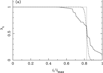
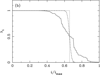
Figure 1: The distribution of eigenvalues of C, shown for symmetric constant latitude cuts of $b_{\mathrm{c}ut}=10$ deg in (a) and $b_{\mathrm{c}ut}=20$ deg in (b). In both panels the eigenvalues are sorted into decreasing order, and distributions are shown for $l_{\mathrm{m}ax}=10$ (solid line), $l_{\mathrm{m}ax}=100$ (dashed line) and $l_{\mathrm{m}ax}=1000$ (dotted line). The limiting cases of $l_{\mathrm{m}ax}\rightarrow\infty$ [in which $\Omega_{{S^{\prime}}}/(4\pi)$ of the eigenvalues are unity and the remaineder zero] are almost indistinguishable from the $l_{\mathrm{m}ax}=1000$ distributions.

The coupling matrix has $i_{\mathrm{m}ax}=(l_{\mathrm{m}ax}+1)^{2}$ eigenvectors, $\mbox{\boldmath${v}$}_{i}$, and eigenvalues, $\lambda_{i}$, which satisfy

$$\mbox{\bf\sf{C}}\mbox{\boldmath${v}$}_{i}=\lambda_{i}\mbox{\boldmath${v}$}_{i}.$$ (5)

Premultiplying by $\mbox{\boldmath${Y}$}^{\mathrm{T}}(\hat{\mbox{\boldmath${r}$}})$ and expanding out the implicit summations gives

$$\int_{{S^{\prime}}}\sum_{k=1}^{i_{\mathrm{m}ax}}Y_{k}(\hat{\mbox{\boldmath${r}$}}^{\prime})(v_{i})_{k}\sum_{j=1}^{i_{\mathrm{m}ax}}Y_{j}(\hat{\mbox{\boldmath${r}$}})Y_{j}(\hat{\mbox{\boldmath${r}$}}^{\prime})\,{\mathrm{d}}\Omega^{\prime}=\lambda_{i}v_{i}(\hat{\mbox{\boldmath${r}$}}),$$ (6)

where $v_{i}(\hat{\mbox{\boldmath${r}$}})=\mbox{\boldmath${Y}$}^{\mathrm{T}}(\hat{\mbox{\boldmath${r}$}})\mbox{\boldmath${v}$}_{i}$ is the $i$th eigenfunction of the coupling matrix. The completeness of the spherical harmonics in the $l_{\mathrm{m}ax}\rightarrow\infty$ limit implies that $\mbox{\boldmath${Y}$}^{\mathrm{T}}(\hat{\mbox{\boldmath${r}$}})\mbox{\boldmath${Y}$}(\hat{\mbox{\boldmath${r}$}}^{\prime})=\delta(\hat{\mbox{\boldmath${r}$}}-\hat{\mbox{\boldmath${r}$}}^{\prime})$ [where $\delta(x)$ is the Dirac delta function], so that equation (6) reduces to

$$\int_{{S^{\prime}}}v_{i}(\hat{\mbox{\boldmath${r}$}}^{\prime})\delta(\hat{\mbox{\boldmath${r}$}}-\hat{\mbox{\boldmath${r}$}}^{\prime})\,{\mathrm{d}}\Omega^{\prime}=\lambda_{i}v_{i}(\hat{\mbox{\boldmath${r}$}}).$$ (7)

For a given $i$ this must be true at all $\hat{\mbox{\boldmath${r}$}}$, which implies that either: $v_{i}(\hat{\mbox{\boldmath${r}$}})=0$ in the cut region, $S-{S^{\prime}}$, in which case $\lambda_{i}=1$; or $v_{i}(\hat{\mbox{\boldmath${r}$}})=0$ in ${S^{\prime}}$, in which case $\lambda_{i}=0$. In other words these eigenfunctions are completely localised in either the cut sphere or the removed region. This bimodality is only strictly true in the $l_{\mathrm{m}ax}\rightarrow\infty$ limit, but, as shown in Fig. 1, is a good approximation for $l_{\mathrm{m}ax}\ga 500$.

As the coupling matrix is symmetric, those eigenvectors with different eigenvalues are orthogonal, and those with the same eigenvalues can be made orthogonal by a rotation in the subspace defined by the eigenvalue in question (e.g. Arfken 1985). Thus the eigenfunctions with $\lambda_{i}=1$ represent an orthogonal basis set on ${S^{\prime}}$, whereas those with $\lambda_{i}=0$ have no support in this region and so cannot be orthogonal (or normalised) on the cut sky. The freedom in choice of basis does not extend to mixing the $\lambda_{i}=0$ modes (i.e. those corresponding to the null-space of C) with the $\lambda_{i}=1$ modes (i.e. those in the range of C), and so the number of supported modes is determined by a combination of the band-limit and the cut.

The number of orthonormal basis functions (i.e. the rank of C) is proportional to the area of the sphere retained, $\Omega_{S^{\prime}}$. Hence it is possible to define only

$$i^{\prime}_{\mathrm{m}ax}\simeq\frac{\Omega_{S^{\prime}}}{\Omega_{S}}i_{\mathrm{m}ax}=\frac{\Omega_{S^{\prime}}}{4\pi}i_{\mathrm{m}ax}$$ (8)

orthonormal functions on the cut sphere for a given (large) band-limit. The relative reduction in the basis set is the same as would occur in the equivalent pixel analysis: the number of pixels retained is also given by $N_{\mathrm{p}}^{\prime}\simeq\Omega_{S^{\prime}}/\Omega_{S}\,N_{\mathrm{p}}$. For low $l_{\mathrm{m}ax}$ these arguments do not hold, and it is possible to create a basis set with more than $\Omega_{S^{\prime}}/\Omega_{S}\,i_{\mathrm{m}ax}$ elements. Moreover, all these functions are required to ensure that the cut-sphere basis set is complete (as well as orthonormal) in the case of a low band-limit.

2.2 Construction of an orthonormal basis

The construction of an orthonormal basis set from a set of linearly-independent functions is a well-established mathematical technique, and a number of orthogonalisation methods are possible. The most basic is Gram-Schmit orthogonalisation (e.g. Arfken 1985), in which the new basis functions are built-up sequentially, but this algorithm is numerically unstable. The modified Gram-Schmidt algorithm (e.g. Golub & van Loan 1996) is stable, but it is generally preferable to use matrix techniques to create all the new basis functions simultaneously.

Starting with the spherical harmonics, $\mbox{\boldmath${Y}$}(\hat{\mbox{\boldmath${r}$}})$, the task is to find a set of functions $\mbox{\boldmath${Y}$}^{\prime}(\hat{\mbox{\boldmath${r}$}})$ which are orthonormal on the incomplete sphere. In terms of a conversion matrix, B, the two sets of functions are related by

$$\mbox{\boldmath${Y}$}^{\prime}(\hat{\mbox{\boldmath${r}$}})=\mbox{\bf\sf{B}}\mbox{\boldmath${Y}$}(\hat{\mbox{\boldmath${r}$}}).$$ (9)

Note that B has dimensions $i^{\prime}_{\mathrm{m}ax}\times i_{\mathrm{m}ax}$, where $i_{\mathrm{m}ax}=(l_{\mathrm{m}ax}+1)^{2}$ and $i^{\prime}_{\mathrm{m}ax}\leq i_{\mathrm{m}ax}$ is determined by the band-limit and the cut, as described in Section 2.1. It is also important to note that the indexing of the $Y^{\prime}_{i}(\hat{\mbox{\boldmath${r}$}})$ is qualitatively different from the $Y_{i}(\hat{\mbox{\boldmath${r}$}})$. The latter are really two-index objects, with their characteristic scale given by $\sim\pi/l$ and $m$ relating to ‘orientation’. However the new basis functions include contributions from spherical harmonics with different $l$-values, and thus do not have a well-defined angular scale. Hence their single index contains no physical information, and the ordering or grouping of the new basis functions is arbitrary.

From equation (1), the coupling matrix of these new functions is

$$\mbox{\bf\sf{C}}^{\prime} = \int_{{S^{\prime}}}\mbox{\boldmath${Y}$}^{\prime}(\hat{\mbox{\boldmath${r}$}}){\mbox{\boldmath${Y}$}^{\prime}}^{\mathrm{T}}(\hat{\mbox{\boldmath${r}$}})\,{\mathrm{d}}\Omega$$ (10)

$$= \mbox{\bf\sf{B}}\mbox{\bf\sf{C}}\mbox{\bf\sf{B}}^{\mathrm{T}}.$$

Hence any conversion matrix which satisfies

$$\mbox{\bf\sf{B}}\mbox{\bf\sf{C}}\mbox{\bf\sf{B}}^{\mathrm{T}}=\tilde{\mbox{\bf\sf{I}}}$$ (11)

yields basis functions which are orthonormal on the cut sphere, and the task of orthogonalisation is reduced to finding a solution for B given C. Whilst such a solution does not exist for arbitrary C, in all cases of practical interest a suitable conversion matrix can be constructed from the coupling matrix. One possible method is direct calculation of the eigenstructure of C, which yields a conversion matrix with elements given by $B_{i^{\prime},i}=(v_{i^{\prime}})_{i}\lambda_{i^{\prime}}^{-1/2}$, where the $\mbox{\boldmath${v}$}_{i^{\prime}}$ are the eigenvectors of C and the $\lambda_{i^{\prime}}$ its positive eigenvalues. However it is advantageous to include the symmetry of the coupling matrix explicitly, which leads to a factorization of the form

$$\mbox{\bf\sf{C}}=\mbox{\bf\sf{A}}\mbox{\bf\sf{A}}^{\mathrm{T}},$$ (12)

where A is an $i_{\mathrm{m}ax}\times i^{\prime}_{\mathrm{m}ax}$ matrix, the form of which is determined by the decomposition method. Combining equations (11) and (12), the task of orthogonalisation is reduced to finding B such that

$$\mbox{\bf\sf{B}}\mbox{\bf\sf{A}}=\tilde{\mbox{\bf\sf{O}}},$$ (13)

where $\tilde{\mbox{\bf\sf{O}}}$ is an $i^{\prime}_{\mathrm{m}ax}\times i^{\prime}_{\mathrm{m}ax}$ orthogonal matrix (i.e. $\tilde{\mbox{\bf\sf{O}}}\tilde{\mbox{\bf\sf{O}}}^{\mathrm{T}}=\tilde{\mbox{\bf\sf{O}}}^{\mathrm{T}}\tilde{\mbox{\bf\sf{O}}}=\tilde{\mbox{\bf\sf{I}}}$).

Whilst equations (12) and (13) are general expressions which must be satisfied by the conversion matrix, they do not define a definite algorithm for the orthogonalisation. In practice it is simplest to choose $\tilde{\mbox{\bf\sf{O}}}=\tilde{\mbox{\bf\sf{I}}}$, leading to the requirement that

$$\mbox{\bf\sf{B}}\mbox{\bf\sf{A}}=\tilde{\mbox{\bf\sf{I}}}.$$ (14)

However the optimal choice of decomposition method used to generate A depends on whether the coupling matrix is (numerically) invertible, and hence on the band-limit of the analysis.

2.2.1 Low-resolution analysis

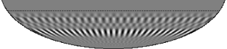
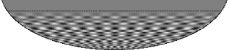
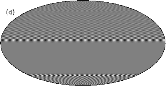
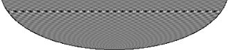
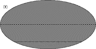
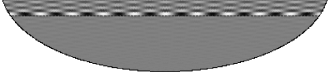
Figure 2: Orthonormal cut sphere basis functions, $Y_{i}^{\prime}(\hat{\mbox{\boldmath${r}$}})$, as described in Section 2.2.2. In all cases $l_{\mathrm{m}ax}=100$, $W_{\mathrm{m}in}=0.01$, and a Mollweide projection is used. The colour-map varies from black (large negative values), through grey (zero), to white (large positive values), in each case being scaled to cover the dynamic range of the relevant basis function. For those in the left column [(a), (c), (e) and (g)] the cut (shown by the dashed lines) is symmetric, with $b_{\mathrm{c}ut}=\pm 20$ deg; for those in the right column [(b), (d), (f) and (h)] the cut (again shown by the dashed lines) is asymmetric, the region between $b_{1}=0$ deg and $b_{2}=-45$ deg having been removed. Within each column the indexing of the basis functions is arbitrary, but they are displayed so that their fractional support in the removed region increases from (a) to (g) and (b) to (h), respectively.

If $l_{\mathrm{m}ax}\la 50$ and most of the sphere is retained (i.e. $\Omega_{S^{\prime}}\ga\Omega_{S}/2=2\pi$) then the coupling matrix is numerically invertible and can be treated as positive definite in practice. Consequently A [defined in equation (12)] is also invertible, and $\mbox{\bf\sf{B}}=\mbox{\bf\sf{A}}^{-1}$, so that, from equation (9), the orthonormal basis set is given by

$$\mbox{\boldmath${Y}$}^{\prime}(\hat{\mbox{\boldmath${r}$}})=\mbox{\bf\sf{A}}^{-1}\mbox{\boldmath${Y}$}(\hat{\mbox{\boldmath${r}$}}).$$ (15)

The form of A depends on the factorization method; of the wide variety available (e.g. Golub & van Loan 1996), the two most useful here are singular value decomposition (SVD) and Cholesky decomposition.

The SVD of the covariance matrix is defined in terms of equation (12) by $\mbox{\bf\sf{A}}=\mbox{\bf\sf{V}}\mbox{\bf\sf{W}}^{1/2}$ (i.e. $\mbox{\bf\sf{C}}=\mbox{\bf\sf{V}}\mbox{\bf\sf{W}}\mbox{\bf\sf{V}}^{\mathrm{T}}$), where V is orthogonal and W is diagonal. The diagonal elements of W are the eigenvalues of C and, as their ordering is arbitrary, W can be defined such that $W_{i,i}\leq W_{i+1,i+1}$, provided the columns of V are permuted in the same way. The columns of V, in turn, are the eigenvectors of C, and V is an orthogonal matrix (i.e. $\mbox{\bf\sf{V}}^{-1}=\mbox{\bf\sf{V}}^{\mathrm{T}}$). Hence the conversion matrix is given by $\mbox{\bf\sf{B}}=\mbox{\bf\sf{A}}^{-1}=\mbox{\bf\sf{W}}^{-1/2}\mbox{\bf\sf{V}}^{\mathrm{T}}$, which is trivially computed once the SVD has been performed. Note that this approach is effectively the same as the direct calculation of the eigenstructure of C mentioned above in Section 2.2.

Whilst SVD is a powerful technique, it is computationally expensive – a Cholesky decomposition is approximately ten times faster, although it can only be performed on symmetric matrices which are numerically positive definite. The Cholesky decomposition of the covariance matrix takes the form $\mbox{\bf\sf{C}}=\mbox{\bf\sf{L}}\mbox{\bf\sf{L}}^{\mathrm{T}}$ (i.e. $\mbox{\bf\sf{A}}=\mbox{\bf\sf{L}}$), where L is lower triangular. Hence the conversion matrix, $\mbox{\bf\sf{B}}=\mbox{\bf\sf{L}}^{-1}$ can be computed quickly from the initial factorization in this case as well. The triangular structure of the conversion matrix also ensures that the new basis functions are the same as those formed by a numerically-stable Gram-Schmidt orthogonalisation (Górski 1994).

Despite the fact that the SVD and the Cholesky decomposition result in quite different sets of basis functions, there is no reason to prefer one over the other in general. In the case of CMB analysis, however, the triangular structure of A and B as generated by the Cholesky decomposition is preferable as it ensures that the non-cosmological monopole and dipole modes are kept separate from the $l\geq 2$ modes, assuming $l$-ordering is used (Górski 1994). If the SVD route is taken (or another indexing scheme used) the separation of the $l=0$ and $l=1$ modes can be ensured using the partial Householder transform described in Appendix C. Nonetheless, if the coupling matrix is sufficiently non-singular, a Cholesky decomposition should be used to create the orthonormal basis set, due to both its computational efficiency and the simplicity with which the non-cosmological modes are handled.

2.2.2 High-resolution analysis

If $l_{\mathrm{m}ax}\ga 50$ the coupling matrix is numerically singular, and thus A [defined in equation (12)] is non-invertible. Cholesky decomposition of C is thus impractical and, whilst an SVD is possible, the conversion matrix as defined in Section 2.2.1 cannot be computed, as the smallest elements of W (i.e. the smallest eigenvalues of C) are so close to zero. This implies that the corresponding columns of V do not contribute to the reconstruction of C and can be ignored. Hence it is possible to perform an approximate SVD of the coupling matrix, defined by $\mbox{\bf\sf{C}}\simeq\tilde{\mbox{\bf\sf{V}}}\tilde{\mbox{\bf\sf{W}}}\tilde{\mbox{\bf\sf{V}}}^{\mathrm{T}}$ (i.e. $\mbox{\bf\sf{A}}=\tilde{\mbox{\bf\sf{V}}}\tilde{\mbox{\bf\sf{W}}}^{1/2}$), where $\tilde{\mbox{\bf\sf{W}}}$ is an $i^{\prime}_{\mathrm{m}ax}\times i^{\prime}_{\mathrm{m}ax}$ diagonal matrix containing the largest elements of W and $\tilde{\mbox{\bf\sf{V}}}$ is an $i^{\prime}_{\mathrm{m}ax}\times i_{\mathrm{m}ax}$ matrix consisting of the corresponding columns of V. The value of $i_{\mathrm{m}ax}$ is determined by the choice of $W_{\mathrm{m}in}$ used to truncate W, but the bimodality of the eigenvalue distribution means that any value between $\sim 10^{-5}$ and $\sim 0.1$ is acceptable. The resultant conversion matrix is $\mbox{\bf\sf{B}}=\tilde{\mbox{\bf\sf{W}}}^{-1/2}\tilde{\mbox{\bf\sf{V}}}^{\mathrm{T}}$ (satisfying $\mbox{\bf\sf{B}}\mbox{\bf\sf{A}}\simeq\tilde{\mbox{\bf\sf{I}}}$) and the $i^{\prime}_{\mathrm{m}ax}$ new basis functions are given by

$$\mbox{\boldmath${Y}$}^{\prime}(\hat{\mbox{\boldmath${r}$}})=\tilde{\mbox{\bf\sf{W}}}^{-1/2}\tilde{\mbox{\bf\sf{V}}}^{\mathrm{T}}\mbox{\boldmath${Y}$}(\hat{\mbox{\boldmath${r}$}}).$$ (16)

These basis functions represent an orthonormal basis set on the incomplete sphere, but they are not formally complete to the nominal band-limit due to the slightly approximate nature of the reduced SVD. The decomposition becomes exact in the limit $l_{\mathrm{m}ax}\rightarrow\infty$ as $\tilde{\mbox{\bf\sf{W}}}\rightarrow\tilde{\mbox{\bf\sf{I}}}$ (from the eigenvalue arguments described in Section 2.1.1) and the reduced SVD becomes $\mbox{\bf\sf{C}}\rightarrow\tilde{\mbox{\bf\sf{V}}}\tilde{\mbox{\bf\sf{V}}}^{\mathrm{T}}$ (i.e. $\mbox{\bf\sf{A}}\rightarrow\tilde{\mbox{\bf\sf{V}}}$ and $\mbox{\bf\sf{B}}\rightarrow\tilde{\mbox{\bf\sf{V}}}^{\mathrm{T}}$) in this limit. Note also that these basis functions are still orthogonal on the full sphere, although they are no longer normalised to unity; this is another potential advantage of the SVD-based method.

Several examples of orthonormal cut-sphere basis functions are shown in Fig. 2, for both symmetric and asymmetric constant latitude cuts. The link between these functions and the spherical harmonics is apparent – they have the same cellular structure, but, for the most part, are combined in such a way that their support is localised to ${S^{\prime}}$. However the functions shown in Fig. 2 (g) and (h) are from the small subset with intermediate values of $W_{i,i}$ and, as such, have considerable support in the removed region.

In the case of CMB analysis, one short-coming of this approach is that the non-cosmological monopole and dipole modes are not distinguished from the higher moments (see Section 3.2), although this separation can be achieved post facto by using a partial Householder transform, as described in Appendix C. In doing this some of the useful properties of the SVD are lost, but this operation need only be performed as the last step in generating the orthonormal basis set, by which stage all the computationally intensive matrix operations have already been performed.

Despite the inconvenience caused by the mixing of the monopole and dipole modes, SVD is clearly the most flexible and general method of orthogonalisation. In part, this stems from the fact that it can be applied to the coupling matrix without any prior knowledge of its singular properties. However, in the high-$l_{\mathrm{m}ax}$ limit, the number of supported basis functions is determined by the area of the cut and given, to a good approximation, by equation (8). Hence faster, if less powerful, techniques can be used to orthogonalise the spherical harmonics for $l_{\mathrm{m}ax}\ga 1000$ as the coupling matrix is guaranteed to have at least $(l_{\mathrm{m}ax}+1)^{2}\Omega_{S^{\prime}}/(4\pi)$ positive eigenvalues. An example of this idea would be to modify the pivoting algorithm in the psuedo-Cholesky decomposition described in Section 4.2.9 of Golub & van Loan (1996) so that the decomposition halts when the predetermined number of basis functions have been generated, as opposed to using the less robust threshold based on the values of the diagonal elements of C.

2.3 Constant latitude cuts

In principle the method presented above is a complete solution to the problem of constructing orthonormal bases on the cut sphere, but the coupling matrix requires $O(l_{\mathrm{m}ax}^{4})$ storage, limiting a general implementation to $l_{\mathrm{m}ax}\simeq 200$ on most current computers. Furthermore, the SVD of an $n\times n$ matrix requires $O(n^{3})$ operations, and so the orthogonalisation operation count scales as $O(l_{\mathrm{m}ax}^{6})$. Similar difficulties are encountered in merely evaluating C, regardless of whether numerical integration or recursive techniques are used (e.g. Hivon et al. 2001).

Fortunately all these difficulties are significantly reduced in the case of a constant latitude cut (cf. Oh, Spergel & Hinshaw 1999; Wandelt et al. 2001), defined by ignoring all $\theta$ for which $\theta_{1}\leq\theta\leq\theta_{2}$. This could be the symmetric removal of the Galactic plane (i.e. $\theta_{1}=\pi/2-b_{\mathrm{c}ut}$ and $\theta_{2}=\pi/2+b_{\mathrm{c}ut}$, where $b_{\mathrm{c}ut}$ is the latitude of the cut) or the absence of data round one pole (i.e. $\theta_{1}=0$ and $\theta_{2}=\theta_{\mathrm{c}ut}$). The formalism derived below can also be trivially extended to include multiple cuts, as would be required for a CMB experiment which did not observe either ecliptic pole.

Explicitly including the constant latitude cut in equation (1), the elements of the coupling matrix are given by

$$C_{i(l,m),i(l^{\prime},m^{\prime})} = \int_{0}^{2\pi}s_{m}(\phi)s_{m^{\prime}}(\phi)\,{\mathrm{d}}\phi$$

$$\times \left[\int^{\cos(\theta_{2})}_{-1}\lambda_{l,|m|}(x)\lambda_{l^{\prime},|m^{\prime}|}(x)\,{\mathrm{d}}x\right.$$

$$+\left.\int_{\cos(\theta_{1})}^{1}\lambda_{l,|m|}(x)\lambda_{l^{\prime},|m^{\prime}|}(x)\,{\mathrm{d}}x\right],$$

where $s_{m}(\phi)$ is defined in equation (44), and the $\lambda_{l,m}(x)$ are normalised associated Legendre functions, given in equation (45). From Appendix A, the first integral in equation (2.3) reduces to $2\pi\delta_{m,m^{\prime}}$, and so

$$C_{i(l,m),i(l^{\prime},m^{\prime})} \!\!\!\!=\!\!\!\! \delta_{m,m^{\prime}}$$

$$\!\!\!\!\times\!\!\!\! \left[\delta_{l,l^{\prime}}-2\pi\int_{\cos(\theta_{2})}^{\cos({\theta_{1}})}\lambda_{l,|m|}(x)\lambda_{l^{\prime},|m|}(x)\,{\mathrm{d}}x\right]\!\!.$$

The remaining integral can be evaluated using a combination of analytical formulæ and recursion relations, as described in Appendix B.

The most important aspect of equation (2.3) is that the coupling matrix C is extremely sparse (only one element in $\sim l_{\mathrm{m}ax}$ is non-zero) and, if stored using the indexing scheme defined in equation (54) (i.e. grouped into sub-matrices of fixed $m$), is block diagonal. C can thus be stored in the form of $2l_{\mathrm{m}ax}+1$ sub-matrices, the $m$th of which has $(l_{\mathrm{m}ax}+1-|m|)^{2}$ elements, and the storage requirements thus scale as $O(l_{\mathrm{m}ax}^{3})$ rather than $O(l_{\mathrm{m}ax}^{4})$. Whilst it is convenient to store all the blocks simultaneously, there is no need to do so, which can further reduce the storage requirements to $O(l_{\mathrm{m}ax}^{2})$. It is also clear from equation (2.3) that only the $m\geq 0$ terms need be treated explicitly and that $l$ and $l^{\prime}$ are interchangeable, decreasing the storage requirements by a further factor of four. Finally, in the case of a symmetric cut (i.e. $\theta_{2}=\pi-\theta_{1}$) the parity of $\lambda_{l,m}(x)$ is such that all terms for which $l+l^{\prime}$ is odd vanish, resulting in an additional halving of the memory requirements.

The orthogonalisation can be performed by decomposing each sub-matrix separately, reducing the operation count from $O(l_{\mathrm{m}ax}^{6})$ to $O(l_{\mathrm{m}ax}^{4})$. The removal of the poorly-supported basis functions is achieved in the same manner as described in Section 2.2, although the book-keeping is more complicated. Similarly the partial Householder transform required to separate the $l=0$ and $l=1$ modes need only be applied to the $m=0$ and $m=\pm 1$ blocks of the resultant conversion matrix (Appendix C). An important side-effect of the separation in $m$ is that the $Y^{\prime}_{i}(\hat{\mbox{\boldmath${r}$}})$ have the same trigonometric $\phi$-dependence as the full-sky spherical harmonics (Appendix A). This also implies that the $Y^{\prime}_{i}(\hat{\mbox{\boldmath${r}$}})$ can be treated as two-index quantities, defined by $m$ and a second, arbitrary index in place of $l$.

The algorithms described here were implemented on the Cambridge Centre for Mathematical Science’s COSMOS 64-processor Silicon Graphics Origin 2000 and the evaluation and decomposition of the coupling matrix at the highest Planck resolution of $l_{\mathrm{m}ax}\simeq$ 2500 required about an hour. The majority of the time was spent factorizing the sub-matrices, and thus significant accelerations are unlikely, the highly-optimised linear algebra package (lapack; Anderson 1992) routines having been used for all the decompositions. For a given choice of $\theta_{1}$ and $\theta_{2}$, the decomposition of C need only be performed once, so orthogonalisation of the spherical harmonics on an incomplete sky should comprise only a small fraction of the analysis required for the forthcoming MAP and Planck missions.

3 Harmonic analysis

Methods for constructing an orthonormal basis set on the incomplete sphere from the spherical harmonics were discussed in Section 2, but in most cases of data analysis it is the harmonic coefficients, representing functions on the sphere, that are of interest. There are at least three useful harmonic expansions of a general function on the sphere, and the relationships between these coefficients, which are summarised in Table LABEL:table:harm, are derived here.

Table 1: Conversions between harmonic coefficients

$\mbox{\boldmath${a}$}=\int_{S}\mbox{\boldmath${Y}$}(\hat{\mbox{\boldmath${r}$}})a(\hat{\mbox{\boldmath${r}$}})\,{\mathrm{d}}\Omega$		$\hat{\mbox{\boldmath${a}$}}=\mbox{\bf\sf{B}}^{\mathrm{T}}\mbox{\bf\sf{B}}\tilde{\mbox{\boldmath${a}$}}\rightarrow\mbox{\bf\sf{C}}^{-1}\tilde{\mbox{\boldmath${a}$}}$	$\hat{\mbox{\boldmath${a}$}}=\mbox{\bf\sf{B}}^{\mathrm{T}}\mbox{\boldmath${a}$}^{\prime}\rightarrow\left(\mbox{\bf\sf{A}}^{\mathrm{T}}\right)^{-1}\mbox{\boldmath${a}$}^{\prime}$
$\tilde{\mbox{\boldmath${a}$}}=\int_{S^{\prime}}\mbox{\boldmath${Y}$}(\hat{\mbox{\boldmath${r}$}})a(\hat{\mbox{\boldmath${r}$}})\,{\mathrm{d}}\Omega$	$\tilde{\mbox{\boldmath${a}$}}=\mbox{\bf\sf{C}}\mbox{\boldmath${a}$}$		$\tilde{\mbox{\boldmath${a}$}}=\mbox{\bf\sf{A}}\mbox{\boldmath${a}$}^{\prime}$
$\mbox{\boldmath${a}$}^{\prime}=\int_{S^{\prime}}\mbox{\boldmath${Y}$}^{\prime}(\hat{\mbox{\boldmath${r}$}})a(\hat{\mbox{\boldmath${r}$}})\,{\mathrm{d}}\Omega$	$\mbox{\boldmath${a}$}^{\prime}=\mbox{\bf\sf{A}}^{\mathrm{T}}\mbox{\boldmath${a}$}$	$\mbox{\boldmath${a}$}^{\prime}=\mbox{\bf\sf{B}}\tilde{\mbox{\boldmath${a}$}}$

The conversions between the various harmonic coefficients defined in Section 3: ${a}$ are the standard coefficients of the spherical harmonics [equation (20)]; $\tilde{\mbox{\boldmath${a}$}}$ are the psuedo-harmonic coefficients [equation (21)]; $\mbox{\boldmath${a}$}^{\prime}$ are the cut-sphere harmonic coefficients [equation (23)]; and $\hat{\mbox{\boldmath${a}$}}$ are the reconstructed spherical harmonic coefficients. The two basis functions are the spherical harmonics, $\mbox{\boldmath${Y}$}(\hat{\mbox{\boldmath${r}$}})$ [defined in Appendix A], and the orthogonalised harmonics, $\mbox{\boldmath${Y}$}^{\prime}(\hat{\mbox{\boldmath${r}$}})$ [defined in Section 2]. If the coupling matrix of the spherical harmonics, C, is invertible, then the expressions for $\hat{\mbox{\boldmath${a}$}}$ following the $\rightarrow$ can be used as exact inversions; otherwise the ‘estimators’ are approximate projections onto the cut region. A can be any matrix such that $\mbox{\bf\sf{A}}\mbox{\bf\sf{A}}^{\mathrm{T}}=\mbox{\bf\sf{C}}$, and B can be any matrix such that $\mbox{\bf\sf{B}}\mbox{\bf\sf{A}}=\tilde{\mbox{\bf\sf{I}}}$.

A band-limited function, $a(\hat{\mbox{\boldmath${r}$}})$, can be completely specified by a finite number of harmonic coefficients as (cf. Appendix A)

$$a(\hat{\mbox{\boldmath${r}$}})=\mbox{\boldmath${Y}$}^{\mathrm{T}}(\hat{\mbox{\boldmath${r}$}})\mbox{\boldmath${a}$},$$ (19)

where it is assumed that $l_{\mathrm{m}ax}$ is greater than or equal to the band-limit of $a(\hat{\mbox{\boldmath${r}$}})$ and the harmonic coefficients are defined by

$$\mbox{\boldmath${a}$}=\int_{S}\mbox{\boldmath${Y}$}(\hat{\mbox{\boldmath${r}$}})a(\hat{\mbox{\boldmath${r}$}})\,{\mathrm{d}}\Omega.$$ (20)

The invertibility of these transformations is due to the orthonormality of the spherical harmonics on $S$ and the fact that they represent a complete basis set given the band-limit.

If $a(\hat{\mbox{\boldmath${r}$}})$ is only known over some fraction of the sphere ${S^{\prime}}\leq S$, then ${a}$ cannot be determined as above, as the integral in equation (20) is incomplete. In this case the psuedo-harmonics

$$\tilde{\mbox{\boldmath${a}$}}=\int_{S^{\prime}}\mbox{\boldmath${Y}$}(\hat{\mbox{\boldmath${r}$}})a(\hat{\mbox{\boldmath${r}$}})\,{\mathrm{d}}\Omega$$ (21)

fully specify $a(\hat{\mbox{\boldmath${r}$}})$ in ${S^{\prime}}$ due to the band-limit. From equation (19) they are related to the full harmonic coefficients by

$$\tilde{\mbox{\boldmath${a}$}}=\mbox{\bf\sf{C}}\mbox{\boldmath${a}$},$$ (22)

where C is the coupling matrix, defined in equation (1).

The psuedo-harmonics are useful quantities, but it is preferable to work with basis functions that are orthonormal on ${S^{\prime}}$. Denoted $\mbox{\boldmath${Y}$}^{\prime}(\hat{\mbox{\boldmath${r}$}})$ in Section 2, their harmonic coefficients are given by

$$\mbox{\boldmath${a}$}^{\prime}=\int_{S^{\prime}}\mbox{\boldmath${Y}$}^{\prime}(\hat{\mbox{\boldmath${r}$}})a(\hat{\mbox{\boldmath${r}$}})\,{\mathrm{d}}\Omega.$$ (23)

The relationship between $\mbox{\boldmath${Y}$}(\hat{\mbox{\boldmath${r}$}})$ and $\mbox{\boldmath${Y}$}^{\prime}(\hat{\mbox{\boldmath${r}$}})$ given in equation (9) flows through to the harmonic coefficients and applying equations (9), (12) and (19) to equation (23) gives

$$\mbox{\boldmath${a}$}^{\prime} = \mbox{\bf\sf{B}}\int_{{S^{\prime}}}\mbox{\boldmath${Y}$}(\hat{\mbox{\boldmath${r}$}})\left[\mbox{\boldmath${Y}$}^{\mathrm{T}}(\hat{\mbox{\boldmath${r}$}})\mbox{\boldmath${a}$}\right]\,{\mathrm{d}}\Omega$$ (24)

$$= {a}$$ BC

$$= \mbox{\bf\sf{A}}^{\mathrm{T}}\mbox{\boldmath${a}$}.$$

The form of the above transformation depends on the decomposition used to generate A (cf. Section 2.2), but, for CMB analysis, it is desirable to separate the non-cosmological modes. This amounts to demanding that the only four of the $a^{\prime}_{i}$ have any contribution from the $l=0$ and $l=1$ spherical harmonic coefficients. The uppper triangular structure of $\mbox{\bf\sf{A}}^{\mathrm{T}}=\mbox{\bf\sf{L}}$ as generated by a Cholesky decomposition inherently satisfies this requirement, but in general the conversion matrix needs to be transformed explicitly. One option is to use successive partial Householder transforms, as described in detail in Appendix C. As can be seen from Fig. 3, the index-ordering and decomposition method combine to give a wide variety of conversion matrices; which of these is most suitable depends on the application.

It is also possible to convert between the psuedo-harmonics and the cut-sky harmonics, as they both contain information about $a(\hat{\mbox{\boldmath${r}$}})$ in ${S^{\prime}}$ alone. Combining equations (12), (21) and (23) implies that $\tilde{\mbox{\boldmath${a}$}}=\mbox{\bf\sf{A}}\mbox{\boldmath${a}$}^{\prime}$ and $\mbox{\boldmath${a}$}^{\prime}=\mbox{\bf\sf{B}}\tilde{\mbox{\boldmath${a}$}}$. However it is not always possible to determine ${a}$ from either $\mbox{\boldmath${a}$}^{\prime}$ or $\tilde{\mbox{\boldmath${a}$}}$. In the low-$l_{\mathrm{m}ax}$ limit these inversions are defined (Section 3.1), but for appreciable band-limits only a projection onto the cut sphere is possible (Section 3.2).

3.1 Low-resolution analysis

If the coupling matrix is numerically non-singular (i.e. $l_{\mathrm{m}ax}\la 50$) then equation (24) can be inverted to give

$$\mbox{\boldmath${a}$}={\left(\mbox{\bf\sf{A}}^{\mathrm{T}}\right)}^{-1}\mbox{\boldmath${a}$}^{\prime}=\mbox{\bf\sf{B}}^{\mathrm{T}}\mbox{\boldmath${a}$}^{\prime},$$ (25)

and equation (21) implies that

$$\mbox{\boldmath${a}$}=\mbox{\bf\sf{C}}^{-1}\tilde{\mbox{\boldmath${a}$}}.$$ (26)

These are specific examples of the fact that a band-limited function is completely defined if it is known over any finite portion of the sphere, and a cut-sky analysis serves no purpose – any apparently localised contaminants infect the entire sky. However any measurement of a field on the sphere is subject to noise which is not band-limited, in which case the application of a cut has the effect of greatly amplifying the noise in the removed region (see Section 4.4), justifying the use of a cut-sky analysis in the low-resolution limit.

3.2 High-resolution analysis

If $l_{\mathrm{m}ax}\ga 50$ and the coupling matrix is numerically singular, it is impossible to reconstruct (even) a band-limited function that is known only on ${S^{\prime}}$. The loss of information about modes constrained to the cut makes it clear that the analysis has the desired effect of removing contaminated (or otherwise problematic) regions, but the most appropriate transformation from the cut-sphere basis to conventional harmonics is less obvious.

A least squares-like approach leads to a definition of the reconstructed full sky coefficients as

$$\hat{\mbox{\boldmath${a}$}}\simeq\mbox{\bf\sf{B}}^{\mathrm{T}}\mbox{\boldmath${a}$}^{\prime}=\left(\mbox{\bf\sf{A}}\mbox{\bf\sf{B}}\right)^{\mathrm{T}}\mbox{\boldmath${a}$}.$$ (27)

Similarly, equation (22) implies that

$$\hat{\mbox{\boldmath${a}$}}\simeq\mbox{\bf\sf{B}}^{\mathrm{T}}\mbox{\bf\sf{B}}\tilde{\mbox{\boldmath${a}$}}=\left(\mbox{\bf\sf{A}}\mbox{\bf\sf{B}}\right)^{\mathrm{T}}\mbox{\boldmath${a}$},$$ (28)

where $(\mbox{\bf\sf{A}}\mbox{\bf\sf{B}})^{\mathrm{T}}$ is a projection operator onto the range of C, which in real space is ${S^{\prime}}$. If $l_{\mathrm{m}ax}\rightarrow\infty$ it is possible to write $\hat{a}(\hat{\mbox{\boldmath${r}$}})=w_{{S^{\prime}}}(\hat{\mbox{\boldmath${r}$}})a(\hat{\mbox{\boldmath${r}$}})$, where $w_{{S^{\prime}}}(\hat{\mbox{\boldmath${r}$}})$ is the sharp window function defined in equation (3).

It is at this point that the subtle distinctions between the use of a discrete cut and a window function become apparent. These results only hold for band-limited functions, but, as defined above, $\hat{a}(\hat{\mbox{\boldmath${r}$}})$ is not band-limited, and so cannot be analysed self-consistently. Whether a discrete cut or an apodizing function is to be preferred depends on the situation in which the incomplete sky analysis is required.

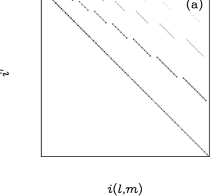
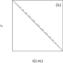
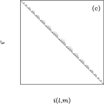
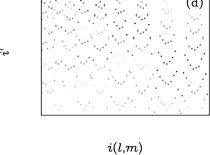
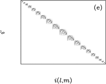
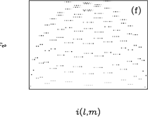
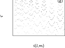
Figure 3: Several examples of the conversion matrices, $\mbox{\bf\sf{A}}^{\mathrm{T}}$, that relate the orthonormal cut sphere harmonic coefficients, $\mbox{\boldmath${a}$}^{\prime}$ to the conventional spherical harmonic coefficients, ${a}$, according to equation (24). In all cases a symmetric, constant latitude of $b_{\mathrm{c}ut}=\pm 20$ deg has been applied and $l_{\mathrm{m}ax}=10$. The row index, $i^{\prime}$, corresponds to the cut-sky harmonic coefficients and the column index, $i(l,m)$, corresponds to the original spherical harmonic coefficients. The colour-map shows the absolute value of the elements of $\mbox{\bf\sf{A}}^{\mathrm{T}}$ varying from zero (white) to their maximum value (black), which is normalised separately in each case. The spherical harmonic coefficients are indexed using $l$-ordering in the left column [(a), (d) and (g)]; $m$-ordering has been used in order to utilise the decoupling of different $m$-modes resulting from the azimuthal symmetry by using block-by-block storage in the central column [(b), (e) and (h)]; and $m$-ordering is used, but the structure of the coupling matrix is not utilised, in the right column [(c) and (f)]. In the case of $l$-ordering the non-cosmological modes are the four left-most columns of the conversion matrix; in the case of $m$-ordering the non-cosmological modes are the left-most columns of the three central blocks. The conversion matrices shown in the top row [(a), (b) and (c)] result from a Cholesky decomposition; those in the middle row [(d), (e) and (f)] are produced by an SVD (in which all modes with $W_{i,i}\leq 0.1$ have been removed); finally, in the bottom row [(g) and (h)], the partial Householder transform described in Appendix C is applied to the conversion matrices shown in the above panels [(d) and (e), respectively].

4 CMB data analysis

In order to determine the properties of the CMB from noisy observations of the microwave sky (Section 4.1) a number of non-trivial analysis steps are required, including: map-making (Section 4.2); component separation (Section 4.3) and power spectrum estimation (Section 4.4). Several algorithms have been suggested for all these steps, and these are discussed briefly below, but the main focus is on when and how to apply a sky cut. Further, whilst it is possible to analyse the data in either real or Fourier space, the latter approach is emphasised here as it is more directly related to the formalism described in Sections 2 and 3, as well as being the focus of a related series of papers (van Leeuwen et al. 2001; Challinor et al. 2001; Stolyarov et al. 2001). Note that the term ‘map’ is used here to denote any representation of a field on the sky and can imply either a set of real space pixel values or a vector of spherical harmonic coefficients.

4.1 Observations

Observations of the CMB can be made using a number of quite distinct techniques. Data have been obtained from the ground, high altitude balloons, and satellites, but the more important distinction is the type of telescope. The experiments listed in Section 1 include: straightforward single dish telescopes, such as BOOMERanG (e.g. Netterfield et al. 2001) and Planck (e.g. Bersanelli et al. 1996); differencing experiments, such as COBE (e.g. Smoot et al. 1992) and MAP (e.g. Jarosik et al. 1998); and interferometers, such as the Cambridge Anisotropy Telescope (CAT; Scott et al. 1996), the Cosmic Backround Imager (CBI; Padin et al. 2001) and the Degree Angular Scale Interferometer (DASI; Halverson et al. 2001). The interferometry surveys inevitably cover only a small fraction of the sky, and so a flat-sky Fourier analysis becomes possible. However the both the differencing and single dish surveys can, in principle, cover most of the celestial sphere, and should yield maps of the microwave sky that are limited only by (the combined effects of) instrument noise and the finite telescope beam.

4.1.1 Noise

The typical receivers used in the above experiments have two main noise contributions: random white noise and a correlated low-frequency (i.e. ‘$1/f$’) component. The latter is potentially troublesome, leading to ‘stripy’ maps with correlated errors, and is the main reason for the popularity of differencing experiments which remove low frequency noise at the moment of observation. However data from single dish surveys can be ‘de-striped’ if the scan strategy includes sufficiently many multiply-observed points (e.g. Tegmark 1997; Delabrouille 1998; Maino et al. 1999) or the time-time noise covariance matrix can be fully included in the map-making process (Wright, Hinshaw & Bennett 1996; Natoli et al. 2001; Challinor et al. 2001). Hence correlated errors are ignored in the simple analysis presented here.

This leaves only the white component, which can be analysed most simply in the case of a single beam experiment. Following Knox (1995), a receiver is characterised by its sensitivity, $s$ (generally chosen to have units of temperature time^1/2). Assuming the noise is Gaussian it has expectation values $\langle n\rangle=0$ and $\langle n^{2}\rangle=s^{2}t$ over an integration time $t$. The manner in which this noise projects onto a sky map depends on the map-making algorithm, the scan strategy, and the beam.

4.1.2 Beam convolution

All telescopes necessarily have a finite point-spread function or beam, which, for a given detector, can be characterised by $b(\hat{\mbox{\boldmath${r}$}})$, the fraction of photons from direction $\hat{\mbox{\boldmath${r}$}}$ that are registered, given a nominal orientation towards the north pole (i.e. $\theta=0$). The harmonic expansion of the beam in this orientation is denoted $\mbox{\boldmath${b}$}=b_{i(l,m)}$, with the band-limit being related to the nominal resolution of the detector. For a given type of telescope the resolution improves with frequency due to diffraction effects; this places limitations on the component separation algorithms that are used on the incomplete sky (Section 4.3).

Most experiments have beams that are manifestly asymmetric, a fact which must be accounted for explicitly by the data analysis algorithms, but the cut-sky issues of interest here can be explored more clearly if the beam is approximated by its azimuthally averaged counterpart (e.g. Challinor et al. 2001). Defined by

$$\bar{b}(\theta)=\frac{1}{2\pi}\int_{0}^{2\pi}b(\theta,\phi)\,{\mathrm{d}}\phi,$$ (29)

its harmonic coefficients are simply

$$\bar{b}_{l,m} = \delta_{m,0}b_{l,0}$$ (30)

$$= \delta_{m,0}\sqrt{(2l+1)\pi}\int_{-1}^{1}\bar{b}\left[\arccos(x)\right]P_{l}(x)\,{\mathrm{d}}x,$$

where $P_{l}(x)$ is a Legendre polynomial (Appendix A). The use of $\bar{b}(\hat{\mbox{\boldmath${r}$}})$ allows the definition of a beam-smoothed sky, $\bar{s}(\hat{\mbox{\boldmath${r}$}})$, given in terms of the true sky, $s(\hat{\mbox{\boldmath${r}$}})$, by

$$\bar{s}(\hat{\mbox{\boldmath${r}$}})=\int_{S}\bar{b}\left[\arccos\left(\hat{\mbox{\boldmath${r}$}}\cdot\hat{\mbox{\boldmath${r}$}}^{\prime}\right)\right]s(\hat{\mbox{\boldmath${r}$}}^{\prime})\,{\mathrm{d}}\Omega^{\prime}.$$ (31)

This convolution is much simpler in harmonic space, and applying equation (48) to equation (31) yields

$$\bar{\mbox{\boldmath${s}$}}=\bar{\mbox{\bf\sf{B}}}\mbox{\boldmath${s}$},$$ (32)

where $\bar{\mbox{\bf\sf{B}}}$ (as distinct from the conversion matrix, B) is a diagonal ‘convolution matrix’ with

$$\bar{B}_{i,i} = \sqrt{\frac{4\pi}{2l(i)+1}}\bar{b}_{l(i),0}$$ (33)

$$= 2\pi\int_{-1}^{1}\bar{b}\left[\arccos(x)\right]P_{l(i)}(x)\,{\mathrm{d}}x,$$

$l(i)$ being defined in Appendix A. The simple form of equation (32) is often utilised explicitly in CMB analysis algorithms (e.g. Knox 1995; Hobson et al. 1998; Oh et al. 1999; Stolyarov 2001), but in all cases full sky coverage is – sometimes implicitly – assumed.

Turning to convolution on the incomplete sphere, ${S^{\prime}}$, application of equation (24) to equation (32) yields

$$\bar{\mbox{\boldmath${s}$}}^{\prime}=\mbox{\bf\sf{A}}^{\mathrm{T}}\bar{\mbox{\bf\sf{B}}}\mbox{\boldmath${s}$},$$ (34)

where A is defined implicitly in equation (12). In the low-resolution limit equation (25) then gives the cut-sky analogue of equation (32) as

$$\bar{\mbox{\boldmath${s}$}}^{\prime}=\bar{\mbox{\bf\sf{B}}}^{\prime}\mbox{\boldmath${s}$}^{\prime},$$ (35)

with the new convolution matrix defined by $\bar{\mbox{\bf\sf{B}}}^{\prime}=\mbox{\bf\sf{A}}^{\mathrm{T}}\bar{\mbox{\bf\sf{B}}}\mbox{\bf\sf{B}}^{\mathrm{T}}$.

For higher band-limits no such relation exists, the loss of modes in the cut region rendering the convolution ill-defined. This is simply understood in real space, as the value of $\bar{s}(\hat{\mbox{\boldmath${r}$}})$ near the edge of ${S^{\prime}}$ is given by an integral that extends several beam widths into the removed region. Thus it is impossible to relate $\bar{s}(\hat{\mbox{\boldmath${r}$}})$ to $s(\hat{\mbox{\boldmath${r}$}})$ with $\hat{\mbox{\boldmath${r}$}}\in{S^{\prime}}$. These arguments are true independent of the representation chosen, but in harmonic space they mean that it is impossible to relate $\bar{\mbox{\boldmath${s}$}}^{\prime}$ to $\mbox{\boldmath${s}$}^{\prime}$.

Whilst equation (35) is formally incorrect in high-$l_{\mathrm{m}ax}$ cases, it is potentially useful as a practical approximation. It is equivalent to assuming that the signal is given by $\mbox{\boldmath${Y}$}^{\prime}(\hat{\mbox{\boldmath${r}$}})\mbox{\boldmath${s}$}^{\prime}$, which implies that $s(\hat{\mbox{\boldmath${r}$}})\simeq 0$ in $S-{S^{\prime}}$. This is particularly inaccurate if the removed region contains anomalously strong sources, such as the Galactic plane. Nonetheless, equation (35) gives $s^{\prime}(\hat{\mbox{\boldmath${r}$}})$ correctly for all $\hat{\mbox{\boldmath${r}$}}$ more than a few beam widths away from the edge of the cut region. However, even if this is an acceptable approximation, there is the further inconvenience that the effective cut-sky beam, $\bar{\mbox{\bf\sf{B}}}^{\prime}$, is not diagonal, introducing couplings between all the modes.

In short, it is preferable to avoid performing any sort of convolution (or deconvolution) on the cut sky, although it is clear that this situation is encountered in any survey with incomplete sky coverage. The one, albeit trivial, exception to this rule is if the beam is a delta function, or at least the closest approximation to a delta function possible given the band-limit under consideration. In this case $\bar{\mbox{\bf\sf{B}}}=\mbox{\bf\sf{I}}$ and hence, from equation (14), $\bar{\mbox{\bf\sf{B}}}^{\prime}=\tilde{\mbox{\bf\sf{I}}}$ as well. Equation (35) then implies that $\bar{\mbox{\boldmath${s}$}}^{\prime}$ ($=\mbox{\boldmath${s}$}^{\prime}$) is the true, unconvolved sky map, estimation of which is addressed next.

4.2 Map-making

Some of the most important products of the next generation of CMB survey will be high-resolution maps of the sky at each of several frequencies. Such maps can be created in a number of ways, but care must be taken to account for a huge variety of systematics whilst retaining as much information as possible. Both real space (e.g. Wright et al. 1996; Bond et al. 1998; Natoli et al. 2001) and Fourier space (van Leeuwen et al. 2001; Challinor et al. 2001) algorithms have been proposed as being suited to particular apsects of the map-making problem. The resultant uncertainties in the pixel values or harmonic coefficients depend on both the data itself (i.e. the scan strategy, noise properties, etc.) and the map-making algorithms used, and can vary quite markedly from experiment to experiment.

Here only the idealised case of uniform sky coverage is considered as the discussion which follows is not significantly changed by this useful simplification. Under this assumption the optimal estimator for the unsmoothed sky, $\hat{\mbox{\boldmath${s}$}}$ ($=\mbox{\boldmath${s}$}+\mbox{\boldmath${n}$}$), would be unbiased (i.e. $\langle\hat{\mbox{\boldmath${s}$}}\rangle=\mbox{\boldmath${s}$}$) and have covariance given by

$$\mbox{\bf\sf{N}}=\left\langle\mbox{\boldmath${n}$}\mbox{\boldmath${n}$}^{\mathrm{T}}\right\rangle=\left\langle\left(\hat{\mbox{\boldmath${s}$}}-\mbox{\boldmath${s}$}\right)\left(\hat{\mbox{\boldmath${s}$}}-\mbox{\boldmath${s}$}\right)^{\mathrm{T}}\right\rangle=\sigma^{2}\bar{\mbox{\bf\sf{B}}}^{-2},$$ (36)

where (cf. Knox 1995) $\sigma^{2}=4\pi s^{2}/(N_{\mathrm{d}}t_{\mathrm{o}bs})$, $t_{\mathrm{o}bs}$ is the total observation time of the survey, and $N_{\mathrm{d}}$ is the number of detectors at the frequency in question (all of which are assumed to have the same beam). An important issue at this point is the band-limit chosen. Clearly only a finite analysis is possible in practice, and $\bar{\mbox{\bf\sf{B}}}$ becomes increasingly singular as $l_{\mathrm{m}ax}\rightarrow\infty$; these two points are related in so far as the sky can never be reconstructed with infinite resolution. The choice of $l_{\mathrm{m}ax}$ is somewhat arbitrary, although any value a factor of a few greater than the effective beam width will ensure that $\bar{\mbox{\bf\sf{B}}}^{-1}$ exists whilst discarding only multipoles that are noise-dominated. The fact that, unlike the useful signal, the noise is not subject to any band-limit is critical to the understanding of the low-$l_{\mathrm{m}ax}$ cut-sky power spectrum estimation discussed in Section 4.4.

Note also that, due to the assumption of uniform sky coverage, the covariance matrix is diagonal. Transforming this estimator into real space yields maps with covariance given by

$$\langle n(\hat{\mbox{\boldmath${r}$}}_{1})n(\hat{\mbox{\boldmath${r}$}}_{2})\rangle=\sigma^{2}\mbox{\boldmath${Y}$}^{\mathrm{T}}(\hat{\mbox{\boldmath${r}$}}_{1})\bar{\mbox{\bf\sf{B}}}^{-2}\mbox{\boldmath${Y}$}(\hat{\mbox{\boldmath${r}$}}_{2}).$$ (37)

As the noise term in the data is not beam-convolved the removal of the beam results in spatial correlations of the noise (as encoded in $\bar{\mbox{\bf\sf{B}}}$), as well as correlations due to the finite resolution analysis (the sums over spherical harmonics), which are essentially equivalent to pixel smoothing. In the more realistic case of non-uniform sky coverage, the covariance matrix is non-diagonal in both bases, a point discussed further by Oh et al. (1999).

The above estimator for the true sky is closely linked to the more commonly used estimator for the smoothed sky, $\hat{\bar{\mbox{\boldmath${s}$}}}$. Being related by $\hat{\bar{\mbox{\boldmath${s}$}}}=\bar{\mbox{\bf\sf{B}}}^{-1}\hat{\mbox{\boldmath${s}$}}$, it is clear they contain the same information (under the assumption of a symmetric beam). The covariance structure of $\hat{\bar{\mbox{\boldmath${s}$}}}$ is simpler as the correlations discussed above are not introduced, but $\hat{\mbox{\boldmath${s}$}}$ is a more natural data object in the context of this discussion as it is the true sky that is of interest. In particular, unsmoothed maps allow more flexibility in applying a sky cut, as the problems with convolution on the incomplete sphere described in Section 4.1.2 do not arise. In practice the best compromise may be to reconstruct the sky convolved with the azimuthally averaged beam, thus creating maps with the simplest covariance structure possible without information loss. This can be done in either real space (e.g. Bond et al. 1998) or harmonic space (Challinor et al. 2001), although the real space pointing matrix is more complicated if beam asymmetry information is included.

In summary, if a survey covers the entire celestial sphere it is preferable to use full-sky frequency maps. However it is possible that small parts of the sky will be missed due to either the scan strategy (cf. Maino et al. 1999) or hardware problems during the survey itself. If this is the case the best unsmoothed map that could be constructed would be larger than the actual observed region, but the errors around the boundary of this area would be very high. An inferential approach is possible, but significant difficulties are encountered, especially in Fourier space (Challinor et al. 2001). Fortunately, it is probable that both MAP and Planck will produce full sky maps at several frequencies, which can then be used to construct maps of the various astrophysical components.

4.3 Component separation

The microwave sky consists of several distinct astrophysical components, as listed in Section 1. Fortunately they have sufficiently distinct spectra that they can be separated using multi-frequency data. Given that MAP and Planck will produce maps in five and ten bands, respectively, it should be possible to produce maps of the various components (particularly the CMB) that are relatively free of contamination. As with map-making, a number of algorithms have been put forward for this stage of the data processing, although the main focus has been on Fourier space methods (e.g. Tegmark & Efstathiou 1996; Hobson et al. 1998; Bouchet & Gispert 1999; Prunet et al. 2001; Stolyarov et al. 2001). Aside from the expected statistical isotropy of the CMB signal, one of the reasons for this emphasis has been the simplicity of beam convolution in harmonic space (Section 4.1.2). This is critical if smoothed frequency maps are used as the effective smoothing scale will vary with frequency if the telescope is (close to) diffraction limited. However if unsmoothed maps are used real space component separation methods (e.g. Baccigalupi et al. 2000) must also come into consideration, the optimal choice of basis being less clear.

One common aspect of all the separation techniques referenced above is that much of the (prior) information about both signal and noise correlations is disregarded in order to render the problem computationally feasible. In real space the correlations between nearby pixels are ignored, and in Fourier space it is the mode-mode couplings that are neglected. Surprisingly, these approximations appear to be unimportant in practice – even the Galactic components have been recovered with striking accuracy. The most relevant result to this discussion is the all-sky component separation to $l_{\mathrm{m}ax}\simeq 2500$ presented by Stolyarov et al. (2001), as it provides clear evidence that whatever correlations are present in the full-sky harmonic basis are unimportant – there are some errors close to the Galactic centre, but they are localised, and there is no sign of this affecting the reconstruction globally.

If the Galactic plane is removed prior to component separation this one troublesome region is no longer present in the analysis, but new problems arise. Firstly, smoothed maps (with frequency-dependent beam-widths) cannot be used as input data without inducing errors around the edges of ${S^{\prime}}$ due to the ill-defined nature of convolution on the cut sky (Section 4.1.2). Even if such errors are deemed acceptable (e.g. Prunet et al. 2001) or beam-deconvolved maps are used, the transformation described in equation (24) completely changes the correlation structure of the harmonics. In particular, the signal-signal correlation matrices are non-diagonal for all components, including random fields like the CMB (see Section 4.4). Whereas the couplings between the spherical harmonic coefficients can apparently be disregarded, this has not been demonstrated for these induced correlations in the orthonormal basis. Prunet et al. (2001) performed cut-sky component separation including them in full, but were thus limited to $l_{\mathrm{m}ax}\simeq 500$, the computational task being made considerably larger.

In real space the application of a cut is trivial, provided that beam-deconvolved maps are used, as it simply requires that pixels in the removed region be ignored. Thus the Baccigalupi et al. (2000) method should be well suited to a cut-sky analysis.

Given that realistic component separation simulations have only recently become available, it is likely that important developments in this field will be made in the near future. For the moment, however, it appears that separation can usefully be performed on either the full or cut sky without introducing catastrophic errors. Provided the models of microwave emissions from the Galactic plane used in the above simulations are sufficiently realistic, it may thus be preferable to generate the full-sky maps of the various astrophysical components, retaining the option of masking unwanted regions at a later stage.

4.4 Power spectrum estimation

If the fluctuations in the early universe were the result of inflation (e.g. Linde 1990) then the CMB is expected to be a Gaussian random field, the statistical properties of which can be specified completely by its angular power spectrum, $C_{l}$. Even if this is not the case, the power spectrum should encode much of the cosmological information present. It is thus unsurprising that, as with map-making and component separation (Sections 4.2 and 4.3, respectively), many different methods of power spectrum estimation have been developed (e.g. Tegmark 1997; Górski 1994; Bond et al. 1998; Oh et al. 1999; Szapudi et al. 2001; Wandelt et al. 2001; Hivon et al. 2001). Further, sky cuts have been incorporated into many of these algorithms as it seems certain that the strength of the Galactic microwave emissions will prevent the CMB from ever being accurately measured in this region. Due to the proliferation of papers on this subject, this discussion of power spectrum estimation is limited to a description of a maximum likelihood formalism using the orthonormal basis functions described in Section 2, with reference to how their behaviour differs in the low- and high-resolution regimes.

4.4.1 Maximum likelihood formalism

The most powerful method of power spectrum estimation is maximum likelihood (e.g. Press et al. 1992), although this has only been implemented to MAP resolution to date (Oh et al. 1999). By invoking Gaussian statistics for both the CMB and the noise, it is possible to write down the exact likelihood for the observed map (e.g. Górski 1994; Borrill 1999). On the full sky the effective data-vector is $\hat{\mbox{\boldmath${s}$}}=\mbox{\boldmath${s}$}+\mbox{\boldmath${n}$}$ (i.e. the estimator for the true sky, of the form discussed in Section 4.2 and not the quantity being estimated here) with the non-cosmological $l=0$ and $l=1$ modes removed. The full likelihood is given by

$$\frac{{\mathrm{d}}p}{{\mathrm{d}}\hat{\mbox{\boldmath${s}$}}}=\frac{1}{\sqrt{(2\pi)^{i_{\mathrm{m}ax}-4}\,\,{\mathrm{d}et}(\mbox{\bf\sf{S}}+\mbox{\bf\sf{N}})}}\exp\left[-\frac{1}{2}\hat{\mbox{\boldmath${s}$}}^{\mathrm{T}}(\mbox{\bf\sf{S}}+\mbox{\bf\sf{N}})^{-1}\hat{\mbox{\boldmath${s}$}}\right],$$

(38)

where S and N are the signal and noise covariance matrices, respectively. The assumption of Gaussianity implies that $S_{i,i^{\prime}}=\delta_{i,i^{\prime}}C_{l(i)}$, where $C_{l}$ is the CMB power spectrum and $l(i)$ is defined in Appendix A. The form of N is determined by a combination of the survey method and the data processing up to this point, but is unlikely to have the simple form of equation (36) due to the imperfect component separation. The maximum likelihood calculation consists of finding an estimator for the underlying power spectrum, $\hat{C_{l}}$, such that equation (38) is maximised, and there are a number of algorithms for finding this quantity (e.g. Bond et al. 1998; Oh et al. 1999).

The maximum likelihood formalism on the cut sky takes the same form as on the full sky, but with the data-vector $\hat{\mbox{\boldmath${s}$}}^{\prime}=\mbox{\bf\sf{A}}^{\mathrm{T}}\hat{\mbox{\boldmath${s}$}}$ and the covariance matrices suitably transformed to give (cf. Górski 1994)

$$\frac{{\mathrm{d}}p}{{\mathrm{d}}\hat{\mbox{\boldmath${s}$}}^{\prime}} = \frac{1}{\sqrt{(2\pi)^{i^{\prime}_{\mathrm{m}ax}-4}{\mathrm{d}et}(\mbox{\bf\sf{S}}^{\prime}+\mbox{\bf\sf{N}}^{\prime})}}$$ (39)

$$\times \exp\left[-\frac{1}{2}\hat{\mbox{\boldmath${s}$}}^{\prime\mathrm{T}}(\mbox{\bf\sf{S}}^{\prime}+\mbox{\bf\sf{N}}^{\prime})^{-1}\hat{\mbox{\boldmath${s}$}}^{\prime}\right],$$

with the four modes containing information on the monopole and dipole (Section 2.2) again excluded. The signal covariance matrix is subject to a simple similarity transform, $\mbox{\bf\sf{S}}^{\prime}=\mbox{\bf\sf{A}}^{\mathrm{T}}\mbox{\bf\sf{S}}\mbox{\bf\sf{A}}$, but the same is not true for the noise covariance matrix as the noise field is not band-limited (a fact critical to the use use of a cut-sky analysis at low resolution, as discussed below). The coupling of the cut-sky modes makes the maximisation of equation (39) non-trivial (cf. Oh et al. 1999), even if $\mbox{\bf\sf{S}}+\mbox{\bf\sf{N}}$ is diagonal on the full sky. Nonetheless it is useful to work under this idealised assumption in order to see how the application of the cut ensures that the maximum likelihood solution is independent of the Galactic signal; the manner in which this is achieved is quite different in the low- and high-resolution cases.

4.4.2 Low-resolution analysis

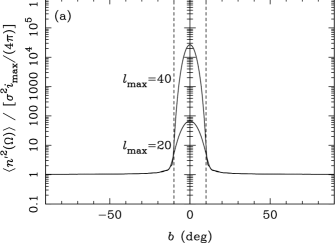
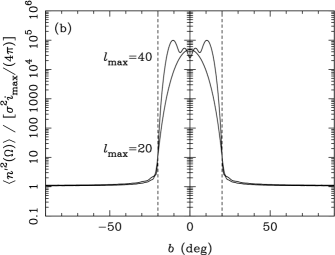
Figure 4: The variance of a (initially) uniform Gaussian noise field as a function of latitude, $b$, after application of the cut-sky orthogonalisation described in Section 3.1. Constant latitude cuts of $b_{\mathrm{c}ut}=10$ deg (a) and $b_{\mathrm{c}ut}=20$ deg (b) were applied (as indicated by the dashed vertical lines) and results are shown for $l_{\mathrm{m}ax}=20$ and $l_{\mathrm{m}ax}=40$, as labelled. (The oscillations near the peak of the latter curve are indicative of the limited accuracy of the decomposition of the ill-conditioned couling matrix.)

The effect of a sky cut on power spectrum estimation is not entirely obvious in the low-$l_{\mathrm{m}ax}$ case in which the coupling matrix (Section 2.1) is invertible. The effective band-limit, produced by the combined effects of the beam and noise (Sections 4 and 4.2), means the signal over the whole sky (including e.g. the Galactic plane) is encoded in the cut-sky coefficients. Thus the application of a cut would be redundant were it not for the presence of non-band-limited noise which cannot be characterised properly a finite harmonic analysis.

Applying the incomplete spherical transform defined in equation (23) to a purely white noise field $n(\hat{\mbox{\boldmath${r}$}})$ [i.e. $\langle n(\hat{\mbox{\boldmath${r}$}})\rangle=0$ and $\langle n(\hat{\mbox{\boldmath${r}$}}_{1})n(\hat{\mbox{\boldmath${r}$}}_{2})\rangle=\delta(\hat{\mbox{\boldmath${r}$}}_{1}-\hat{\mbox{\boldmath${r}$}}_{2})\sigma^{2}$; cf. equation (37)] gives cut-sky harmonic coefficients with $\langle\mbox{\boldmath${n}$}^{\prime}\rangle=\mbox{\boldmath${0}$}$ and

$$\mbox{\bf\sf{N}}^{\prime}=\langle\mbox{\boldmath${n}$}^{\prime}{\mbox{\boldmath${n}$}^{\prime}}^{\mathrm{T}}\rangle=\sigma^{2}\tilde{\mbox{\bf\sf{I}}}.$$ (40)

Projecting back into real space gives a field $n^{\prime}(\hat{\mbox{\boldmath${r}$}})$ which satisfies $\langle n^{\prime}(\hat{\mbox{\boldmath${r}$}})\rangle=0$ and

$$\langle n^{\prime}(\hat{\mbox{\boldmath${r}$}}_{1})n^{\prime}(\hat{\mbox{\boldmath${r}$}}_{2})\rangle=\sigma^{2}\mbox{\boldmath${Y}$}^{\mathrm{T}}(\hat{\mbox{\boldmath${r}$}}_{1})\mbox{\bf\sf{C}}^{-1}\mbox{\boldmath${Y}$}(\hat{\mbox{\boldmath${r}$}}_{2}).$$ (41)

On the full sky the same procedure (i.e. a finite spherical harmonic analysis followed by a transformation back into real space) would yield a noise field with covariance structure given by

$$\langle\hat{n}(\hat{\mbox{\boldmath${r}$}}_{1})\hat{n}(\hat{\mbox{\boldmath${r}$}}_{2})\rangle = \sigma^{2}\mbox{\boldmath${Y}$}^{\mathrm{T}}(\hat{\mbox{\boldmath${r}$}}_{1})\mbox{\boldmath${Y}$}(\hat{\mbox{\boldmath${r}$}}_{2})$$ (42)

$$= \frac{\sigma^{2}}{4\pi}\sum_{l=0}^{l_{\mathrm{m}ax}}(2l+1)P_{l}(\hat{\mbox{\boldmath${r}$}}_{1}\cdot\hat{\mbox{\boldmath${r}$}}_{2}),$$

where $P_{l}(x)$ is a Legendre polynomial (Appendix A). Taking the limit $\hat{\mbox{\boldmath${r}$}}_{2}\rightarrow\hat{\mbox{\boldmath${r}$}}_{1}$ this implies that $\langle\hat{n}^{2}(\hat{\mbox{\boldmath${r}$}})\rangle=i_{\mathrm{m}ax}\sigma^{2}/(4\pi)$, which represents smoothing relative to the original noise field caused by the use of a finite analysis.

Whilst this smoothing occurs in both the cut- and full-sky formalisms, the presence of $\mbox{\bf\sf{C}}^{-1}$ in the former case [equation (41)] implies a spatial dependence. As can be seen from Fig. 4, the noise in the cut region is greatly increased, which is a natural way of formally encoding the qualitative fact that, for whatever reason, the data in the cut is contaminated by more than just the white noise field. Thus, despite the invertibility of the coupling matrix (and the band-limited cut-sky analysis), the application of a cut has the desired effect of greatly reducing the impact of any spurious signal, such as the Galaxy. However Fig. 4 also implies that a similar effect could be achieved without performing a cut (and hence leaving the signal unchanged), instead adding a high level of artificial noise in the offending region(s). Finally, it is important to note that the dual assumptions used in the derivation of equation (41) – uniform noise and no beam – are unrealistic, but the manner in which a low-resolution cut-sky analysis works is the same in less idealised scenarios.

4.4.3 High-resolution analysis

The high-resolution case is more straightforward, as the application of the cut results in a data-vector, $\hat{\mbox{\boldmath${s}$}}^{\prime}$, which contains little information about the removed region. This is quite distinct from the low-resolution case discussed above, in that here it is the predominantly the signal that is changed, rather than the noise. That said, the noise close to the boundary of the cut is increased in the same manner as explained above. This has the same effect as the apodizing function formalism described by Tegmark (1997), downweighting points around which there is not full correlation information.

Another difference between the low- and high-resolution analyses is that $\hat{\mbox{\boldmath${s}$}}^{\prime}$ is smaller than $\hat{\mbox{\boldmath${s}$}}$, from Section 2.1.1. Although this does not result in any significant computational saving, it serves to emphasise the information loss associated with removing part of the sky, and is an independent derivation of the fact that the uncertainties in the estimated power spectrum increase as $4\pi/\Omega_{S^{\prime}}$ (cf. Hobson & Magueijo 1996; Tegmark 1997).

5 Conclusions

The upcoming microwave surveys will require a cut-sky analysis to prevent the strong Galactic emissions from contaminating the CMB signal. The spherical harmonics are non-orthogonal on the cut-sphere, but an orthonormal basis set can be constructed from them using SVD-based techniques (Section 2). The application of the resultant conversion matrix to the conventional multipoles results in cut-sphere harmonics that contain only the desired information. In the low-resolution case the influence of the Galaxy is reduced by increasing the effective noise in the cut; in the high-resolution limit the orthonormal basis functions can model the infinitely sharp cut sufficiently well that they have no support in the removed region. It is also important to note that the cut should probably only be applied after beam-deconvolution has been attempted, as convolution is ill-defined on the incomplete sphere.

The algorithms described here were implemented to Legendre multipoles of $l_{\mathrm{m}ax}\simeq 2500$ for a constant latitude cut, in which case the coupling matrix of the spherical harmonics is block-diagonal. At present computational limitations make a general orthogonalisation impractical for $l_{\mathrm{m}ax}\ga 200$, although there are some possibilities to extend this. For instance only $\sim 1$ per cent of the coupling matrix contains significant information if the cut is well-chosen (e.g. rectangular in $\theta$ and $\phi$) and so sparse matrix techniques should thus allow orthogonalisation to $l_{\mathrm{m}ax}\simeq 1000$ in this case.

Another requirement is orthogonalisation of tensor basis functions on the incomplete sphere, as both the MAP and Planck satellites will measure polarization. The resultant formalism is more complicated, but the same general principles hold; this issue is explored further by Lewis, Challinor & Turok (2001).

Appendix A Spherical harmonics

The spherical harmonics form a complete set of orthonormal basis functions over the entire sphere. They are most commonly defined as complex functions (e.g. Landau & Lifshitz 1976; Brink & Satchler 1993), but it is more convenient to use real harmonics in this application. Adapting the notation of Górski (1994), the real spherical harmonics are given by

$$Y_{l,m}(\hat{\mbox{\boldmath${r}$}})=Y_{l,m}(\theta,\phi)=\lambda_{l,|m|}[\cos(\theta)]s_{m}(\phi),$$ (43)

where $l\geq 0$ and $|m|\leq l$ and

$$s_{m}(\phi)=\left\{\begin{array}[]{lll}\sqrt{2}\sin(|m|\phi),&{\mathrm{i}f}&m<0,\\ \\ 1,&{\mathrm{i}f}&m=0,\\ \\ \sqrt{2}\cos(|m|\phi),&{\mathrm{i}f}&m>0,\end{array}\right.$$ (44)

implying that $\int_{0}^{2\pi}s_{m}(\phi)s_{m^{\prime}}(\phi)\,{\mathrm{d}}\phi=2\pi\delta_{m,m^{\prime}}$. For $0\leq m\leq l$ and $-1\leq x\leq 1$ the normalised associated Legendre functions are defined by

$$\lambda_{l,m}(x)=\sqrt{\frac{2l+1}{4\pi}\frac{(l-m)!}{(l+m)!}}P_{l,m}(x).$$ (45)

Hence $\int_{-1}^{1}\lambda_{l,m}(x)\lambda_{l^{\prime},m}(x)\,{\mathrm{d}}x=\delta_{l,l^{\prime}}/(2\pi)$. Under the same conditions the (unnormalised) associated Legendre functions are given by

$$P_{l,m}(x)=(-1)^{m}\left(1-x^{2}\right)^{m/2}\frac{{\mathrm{d}}^{m}}{{\mathrm{d}}x^{m}}P_{l}(x),$$ (46)

with the Legendre polynomials given by

$$P_{l}(x)=\frac{(-1)^{l}}{2^{l}l!}\frac{{\mathrm{d}}^{l}}{{\mathrm{d}}x^{l}}\left(1-x^{2}\right)^{l}.$$ (47)

A real field on the sphere, $a(\hat{\mbox{\boldmath${r}$}})$, can be expanded in terms of spherical harmonic coefficients, given by

$$a_{l,m}=\int_{S}Y_{l,m}(\hat{\mbox{\boldmath${r}$}})a(\hat{\mbox{\boldmath${r}$}})\,{\mathrm{d}}\Omega.$$ (48)

This can be inverted to give

$$a(\hat{\mbox{\boldmath${r}$}})=\sum_{l=0}^{l_{\mathrm{m}ax}}\sum_{m=-l}^{l}a_{l,m}Y_{l,m}(\hat{\mbox{\boldmath${r}$}}),$$ (49)

provided that $l_{\mathrm{m}ax}\rightarrow\infty$, due to the orthonormality of the spherical harmonics on the full sphere:

$$\int_{S}Y_{l,m}(\hat{\mbox{\boldmath${r}$}})Y_{l^{\prime},m^{\prime}}(\hat{\mbox{\boldmath${r}$}})\,{\mathrm{d}}\Omega=\delta_{l,l^{\prime}}\delta_{m,m^{\prime}}.$$ (50)

If a finite $l_{\mathrm{m}ax}$ is used this inversion is no longer possible for general $a(\hat{\mbox{\boldmath${r}$}})$, although it does still hold for band-limited functions.

Whilst the two indices $l$ and $m$ have quite distinct interpretations it is convenient to combine them into a single index, $i$, which allows the definition of vectors $\mbox{\boldmath${Y}$}(\hat{\mbox{\boldmath${r}$}})=Y_{i(l,m)}(\hat{\mbox{\boldmath${r}$}})$ and $\mbox{\boldmath${a}$}=a_{i(l,m)}$. Two obvious indexing schemes present themselves: grouping in $l$ and $m$. The first, as introduced by Górski (1994), is natural for power spectrum estimation and very simple:

$$i(l,m)=l^{2}+l+m+1.$$ (51)

The two ‘inverses’ of this relationship are

$$l={\mathrm{i}nt}\,\left[(i-1)^{1/2}\right]$$ (52)

and

$$m=i-(l^{2}+l+1).$$ (53)

The second choice of ordering is useful in cases of azimuthal symmetry in which the orthogonality expressed in equation (44) is maintained, and grouping in $m$ is achieved by defining

$$i(l,m)=\left\{\begin{array}[]{lll}l+m+1\\ \mbox{}+(l_{\mathrm{m}ax}+m)(l_{\mathrm{m}ax}+m+1)/2,&{\mathrm{i}f}&m\leq 0,\\ \\ l-l_{\mathrm{m}ax}+(l_{\mathrm{m}ax}+1)^{2}\\ \mbox{}-(l_{\mathrm{m}ax}-m)(l_{\mathrm{m}ax}-m+1)/2,&{\mathrm{i}f}&m>0.\end{array}\right.$$

(54)

The ‘inverses’ in this case are given by

$$m=\left\{\begin{array}[]{lll}\lx@intercol\!\!\!\!{\mathrm{i}nt}\left[-l_{\mathrm{m}ax}+\frac{1}{2}\left(\sqrt{8i+1}-3\right)\right],\hfil\lx@intercol\\ \lx@intercol\hfil\,\,\,\,\,\,\,{\mathrm{if}}\,\,\,\,\,\,\,i\leq(l_{\mathrm{m}ax}+1)(l_{\mathrm{m}ax}+2)/2,\lx@intercol\\ \\ \lx@intercol\!\!\!\!{\mathrm{i}nt}\left[\!\!\left[l_{\mathrm{m}ax}-\frac{1}{2}\left\{\sqrt{8[(l_{\mathrm{m}ax}+1)^{2}-i+1]+1}-3\right\}\right]\!\!\right],\hfil\lx@intercol\\ \lx@intercol\hfil\,\,\,\,\,\,\,{\mathrm{if}}\,\,\,\,\,\,\,i>(l_{\mathrm{m}ax}+1)(l_{\mathrm{m}ax}+2)/2\lx@intercol\end{array}\right.$$

(55)

and

$$l=\left\{\begin{array}[]{lll}i-\left[m+1\right.\\ \mbox{}\left.+(l_{\mathrm{m}ax}+m)(l_{\mathrm{m}ax}+m+1)/2\right],&{\mathrm{i}f}&m\leq 0,\\ \\ i-\left[-l_{\mathrm{m}ax}+(l_{\mathrm{m}ax}+1)^{2}\right.\\ \mbox{}\left.-(l_{\mathrm{m}ax}-m)(l_{\mathrm{m}ax}-m+1)/2\right],&{\mathrm{i}f}&m>0.\end{array}\right.\!\!\!\!\!\!\!$$ (56)

Other indexing schemes have been used in the more specific case of simulated Planck data-sets in which the sky coverage is periodic in azimuth (van Leeuwen, private communication), but are beyond the scope of this paper.

Appendix B Integration of products of associated Legendre functions

In Section 2.3 integrals of the form

$$I_{l,l^{\prime},m}(x_{1},x_{2})=\int_{x_{1}}^{x_{2}}\lambda_{l,m}(x)\lambda_{l^{\prime},m}(x)\,{\mathrm{d}}x$$ (57)

arose; here the $\lambda_{l,m}(x)$ are the normalised associated Ledengre functions, defined in equation (45), and $m$ is assumed to be non-negative. These integrals can be evaluated quickly and accurately using a combination of closed formulæ and recursion relations.

The associated Legendre functions, $P_{l,m}(x)$ [defined in equation (46)], are solutions of the ordinary differential equation (e.g. Arfken 1985)

$$\frac{{\mathrm{d}}}{{\mathrm{d}}x}\!\!\left[\left(1-x^{2}\right)\frac{{\mathrm{d}}P_{l,m}}{{\mathrm{d}}x}\right]+\left[l(l+1)-\frac{m^{2}}{1-x^{2}}\right]P_{l,m}(x)=0.$$ (58)

Multiplying this equation by $P_{l^{\prime},m}(x)$ and integrating (from $x_{1}$ to $x_{2}$) by parts twice yields

$$(l-l^{\prime})(l+l^{\prime}+1)\int_{x_{1}}^{x_{2}}P_{l,m}(x)P_{l^{\prime},x}(x)\,{\mathrm{d}}x$$ (59)

$$=\!\!\!\left.\left[\!\!\left(1-x^{2}\right)P_{l,m}(x)\frac{{\mathrm{d}}P_{l^{\prime},m}}{{\mathrm{d}}x}-\left(1-x^{2}\right)P_{l^{\prime},m}(x)\frac{{\mathrm{d}}P_{l,m}}{{\mathrm{d}}x}\right]\!\right|_{x=x_{1}}^{x=x_{2}}.$$

This is a reflection of the standard result that integrals of solutions of a self-adjoint differential equation [as equation (58) is] can be expressed as boundary terms (e.g. Arfken 1985). The derivatives in equation (59) can be removed by using the standard recursion relationship (e.g. Gradshteyn & Ryzhik 2000)

$$\left(1-x^{2}\right)\frac{{\mathrm{d}}P_{l,m}}{{\mathrm{d}}x}=(l+m)P_{l-1,m}(x)-lxP_{l,m}(x)$$ (60)

to yield, for $l\neq l^{\prime}$,

$$\int_{x_{1}}^{x_{2}}P_{l,m}(x)P_{l^{\prime},x}(x)\,{\mathrm{d}}x=\frac{1}{(l-l^{\prime})(l+l^{\prime}+1)}$$

$$\times \left[(l^{\prime}+m)P_{l,m}(x)P_{l^{\prime}-1,m}(x)\right.$$ (61)

$$+(l-l^{\prime})xP_{l,m}(x)P_{l^{\prime},m}(x)$$

$$\left.\left.-(l+m)P_{l-1,m}(x)P_{l^{\prime},m}(x)\right]\right|_{x=x_{1}}^{x=x_{2}}.$$

Note that the first term must be omitted if $l^{\prime}=m$ and that the third term must be omitted if $l=m$; these Legendre functions are implicitly zero from equation (46). Finally, this can be normalised according to equation (45), giving

$$I_{l,l^{\prime},m}(x_{1},x_{2})=\frac{1}{(l-l^{\prime})(l+l^{\prime}+1)}$$ (62)

$$\times \left[\sqrt{\frac{2l^{\prime}+1}{2l^{\prime}-1}(l^{2}-m^{2})}\lambda_{l,m}(x)\lambda_{l^{\prime}-1,m}(x)\right.$$

$$\mbox{}+(l-l^{\prime})x\lambda_{l,m}(x)\lambda_{l^{\prime},m}(x)$$

$$\left.\left.-\sqrt{\frac{2l+1}{2l-1}(l^{2}-m^{2})}\lambda_{l-1,m}(x)\lambda_{l^{\prime},m}(x)\right]\right|_{x=x_{1}}^{x=x_{2}}.$$

An alternative derivation of this result was presented by Wandelt et al. (2001); it is also in principle equivalent to Eq. 5.9(13) of Varshalovich, Moskalev & Khersonskii (1988), but their application of equation (60) is in error.

For the case $l=l^{\prime}$ a recursion relation is required, starting with $l=m$. Combining equations (45) and (46),

$$\lambda_{m,m}(x)=(-1)^{m}\sqrt{\frac{2m+1}{4\pi}}(2m-1)!!\left(1-x^{2}\right)^{m/2},$$ (63)

where $n!!=1\times 3\times\cdots\times(n-2)\times n$ for odd $n$. Integrating by parts and using equation (63) again gives

$$I_{m,m,m}(x_{1},x_{2})$$ (64)

$$\mbox{}=\left\{\begin{array}[]{lll}\frac{x_{2}-x_{1}}{4\pi},&{\mathrm{i}f}&m=0,\\ \\ I_{m-1,m-1,m-1}(x_{1},x_{2})+\frac{\left.x\lambda_{m,m}^{2}(x)\right|_{x_{1}}^{x_{2}}}{2m+1},&{\mathrm{i}f}&m>0.\end{array}\right.$$

Moving to $l=m+1$, the standard relationship (e.g. Gradshteyn & Ryzhik 2000) that

$$\lambda_{m+1,m}(x)=(2m+3)x\lambda_{m,m}(x)$$ (65)

combines with equation (63) to give

$$I_{m+1,m+1,m}(x_{1},x_{2}) = I_{m,m,m}(x_{1},x_{2})$$ (66)

$$- \frac{2m+2}{2m+3}\left.x\,\lambda^{2}_{m+1,m+1}(x)\right|_{x_{1}}^{x_{2}},$$

where the first term is given in equation (64).

The last step is to derive a recursion relation relating $I_{l,l,m}(x_{1},x_{2})$ to $I_{l-1,l-1,m}(x_{1},x_{2})$ and $I_{l-2,l-2,m}(x_{1},x_{2})$. Eq. (C22) of Wandelt et al. (2001) gives a four-term recursion to obtain $I_{l,l^{\prime},m}(x_{1},x_{2})$; it can be applied successively (once swapping $l$ and $l^{\prime}$) to obtain

$$I_{l,l,m}(x_{1},x_{2})=-\frac{2m^{2}-2l^{2}+2l-1}{(l-m)(l+m)}I_{l-1,l-1,m}(x_{1},x_{2})$$

$$- \frac{(l-1-m)(l-1+m)}{(l-m)(l+m)}I_{l-2,l-2,m}(x_{1},x_{2})$$

$$- \sqrt{\frac{2l-1}{2l+1}\frac{1}{(l-m)(l+m)}}$$

$$\times\left.\left(1-x^{2}\right)\lambda_{l,m}(x)\lambda_{l-1,m}(x)\right|_{x=x_{1}}^{x=x_{2}}$$

$$+ \sqrt{\frac{2l-1}{2l-3}\frac{(l-1-m)(l-1+m)}{(l-m)^{2}(l+m)^{2}}}$$

$$\times\left.\left(1-x^{2}\right)\lambda_{l-1,m}(x)\lambda_{l-2,m}(x)\right|_{x=x_{1}}^{x=x_{2}}.$$

In summary, equation (62) can be used to evaluate all $I_{l,l^{\prime},m}(x_{1},x_{2})$ for which $l\neq l^{\prime}$, and equations (64), (66) and (B) combine to give all $I_{l,l,m}(x_{1},x_{2})$ recursively.

Appendix C Treatment of non-cosmological modes

All the cosmological information encoded in the CMB is expected to be contained in the $l\geq 2$ modes; the $l=0$ mode in an isotropic universe can be normalised arbitrarily and the $l=1$ modes can be set to zero by adopting an appropriate reference frame. Nonetheless, observations of the microwave sky will yield non-zero monopole and dipole values for a number of reasons (e.g. the observer’s motion; Galactic emission; extra-Galactic point-sources). Hence these low-order modes must be included in the analysis of CMB data, but should be kept separate from the cosmological modes, as is naturally the case if spherical harmonic coefficients are used to describe the data. It is also important to note that the properties of the basis functions themselves are unimportant – the essential requirement is that only four of the cut-sky harmonic coefficients contain information on the unwanted modes.

The method of orthogonalisation summarised in equations (11), (12) and (14) does not explicitly impose any particular structure on the conversion matrix, A [which relates harmonic coefficients on the incomplete sphere to those on the full sphere by $\mbox{\boldmath${a}$}^{\prime}=\mbox{\bf\sf{A}}^{\mathrm{T}}\mbox{\boldmath${a}$}$; equation (24)]. The non-cosmological modes are kept separate from the cosmological modes if the first four columns of $\mbox{\bf\sf{A}}^{\mathrm{T}}$ have only zeros from the fifth row on, assuming the full-sky harmonic coefficients are indexed using $l$-ordering (Appendix A). This is achieved naturally if $\mbox{\bf\sf{A}}^{\mathrm{T}}$ is constructed to be upper triangular, as in the case of the Cholesky decomposition described in Section 2.2.1. The other decomposition methods discussed in Section 2.2 do not share this property, and so the resultant conversion matrices must be adjusted explicitly.

One way of achieving this is to use a partial Householder transform (e.g. Press et al. 1992). The last $i^{\prime}_{\mathrm{m}ax}-i$ elements of the $i$th column of a general $i^{\prime}_{\mathrm{m}ax}\times i_{\mathrm{m}ax}$ matrix can be set to zero by the transformation $\mbox{\bf\sf{M}}^{\prime}=\mbox{\bf\sf{P}}_{i}\mbox{\bf\sf{M}}$, with the orthogonal Householder matrix defined by

$$\mbox{\bf\sf{P}}_{i}=\tilde{\mbox{\bf\sf{I}}}-2\frac{\mbox{\boldmath${m}$}_{i}\mbox{\boldmath${m}$}_{i}^{\mathrm{T}}}{\mbox{\boldmath${m}$}_{i}^{\mathrm{T}}\mbox{\boldmath${m}$}_{i}},$$ (67)

where $\mbox{\boldmath${m}$}_{i}$ is given by

$$(m_{i})_{j}=\left\{\begin{array}[]{lll}0,&{\mathrm{i}f}&j<i,\\ &&\\ M_{j,i}+\sqrt{\sum_{k=i}^{i^{\prime}_{\mathrm{m}ax}}M_{k,i}^{2}},&{\mathrm{i}f}&j=i,\\ &&\\ M_{j,i},&{\mathrm{i}f}&j>i,\end{array}\right.$$ (68)

and $i\leq\min(i^{\prime}_{\mathrm{m}ax},i_{\mathrm{m}ax}$) is assumed. Provided that the Householder matrix applied to B is that generated from $\mbox{\bf\sf{A}}^{\mathrm{T}}$, the transformations ${\mbox{\bf\sf{A}}^{\prime}}^{\mathrm{T}}=\mbox{\bf\sf{P}}_{i}\mbox{\bf\sf{A}}^{\mathrm{T}}$ and $\mbox{\bf\sf{B}}^{\prime}=\mbox{\bf\sf{P}}_{i}\mbox{\bf\sf{B}}$ leave equations (12) and (14) unaffected as $\mbox{\bf\sf{P}}_{i}$ is orthogonal by construction. Applying $\mbox{\bf\sf{P}}_{1}$, $\mbox{\bf\sf{P}}_{2}$, $\mbox{\bf\sf{P}}_{3}$ and then $\mbox{\bf\sf{P}}_{4}$ to the successively updated $\mbox{\bf\sf{A}}^{\mathrm{T}}$ ensures that the $l=0$ and $l=1$ modes influence only the first four cut-sky harmonic coefficients, as required. This procedure could be continued, moving $\mbox{\bf\sf{A}}^{\mathrm{T}}$ successively closer to upper triangular form, although this cannot be achieved in full as $\mbox{\bf\sf{A}}^{\mathrm{T}}$ has more columns than rows.

Special mention must be made of the constant latitude cut case, the symmetry of which can only be utilised if the spherical harmonics are indexed using $m$-ordering (Appendix A). In this case only the $m=0$ and $m=\pm 1$ blocks have any contribution from the monopole or dipole, and each can be treated separately. Further, the ordering within these blocks is such that the non-cosmological modes are in the first rows, and so the above algorithm can be applied to each of three blocks as is. The only slight inconvenience is that it is no longer the first four cut-sky modes that contain the non-cosmological information, and the relevant modes must be flagged explicitly.

References

- [Abramowitz & Stegun 1971] Abramowitz M., Stegun I. A., 1971, Handbook of Mathematical Functions (9th ed.). Dover Publications, New York
- [Anderson et al. 1992] Anderson E., et al., 1992, Lapack User’s Guide. Soc. for Indust. and App. Math., Philadelphia
- [Arfken 1985] Arfken G., 1985, Mathematical Methods for Physicists (3rd ed.). Academic Press, Boston
- [Baccigalupi et al. 2000] Baccigalupi C., et al., 2000, MNRAS, 318, 769
- [Barreiro 2000] Barreiro R. B., 2000, New Ast. Rev., 44, 179
- [Bennett et al. 1992] Bennett C. L., et al., 1992, ApJ, 396, L7
- [Bersanelli et al. 1996] Bersanelli M., et al., 1996, COBRAS/SAMBA, The Phase A Study for an ESA M3 Mission. ESA Report D/SCI(96)3
- [Birkinshaw 1999] Birkinshaw M., 1999, Phys. Rep., 310, 97
- [Bond et al. 1998] Bond J. R., Jaffe A. H., Knox L., 1998, Phys. Rev. D, 57, 2117
- [Borrill 1999] Borrill J., 1999, in Maiani L., Mechiorri F., Vittorio N., eds., 3K Cosmology: EC-TMR Conference. American Institute of Physics, New York, p. 277
- [Brink & Satchler 1993] Brink D. M., Satchler G. R., 1993, Angular Momentum (3rd ed.). Clarendon Press, Oxford
- [Bouchet & Gispert 1999] Bouchet, F. R., Gispert, R., 1999, New Ast., 4, 443
- [Challinor et al. 2001] Challinor A. D., Mortlock D. J., van Leeuwen F., Lasenby A. N., Hobson M. P., Ashdown M. A. J., Efstathiou, G. P., 2001, MNRAS, submitted
- [Coble et al. 1999] Coble K., et al., 1999, ApJ, 519, L5
- [de Bernardis et al. 2000] de Bernardis P., et al., 2000, Nature, 404, 955
- [Delabrouille 1998] Delabrouille J., 1998, A&AS, 127, 555
- [de Oliveira-Costa et al. 1997] de Oliveira-Costa A., Kogut A., Devline M. J., Netterfield C. B., Page L. A., Wollack E. J., 1997, ApJ, 482, L17
- [Efstathiou et al. ef99] Efstathiou G., Bridle S. L., Lasenby A. N., Hobson M. P., Ellis R. S., 1999, MNRAS, 303, L47
- [Golub & van Loan 1996] Golub G. H., van Loan C. F., 1996, Matrix Computations (3rd ed.). The Johns Hopkins Univ. Press, Baltimore
- [Górski 1994] Górski K. M., 1994, ApJ, 430, L85
- [Górski et al. 1994] Górski K. M., et al., 1994, ApJ, 430, L89
- [Gradshteyn & Ryzhik 2000] Gradshteyn I. S., Ryzhik I. M., 2000, Table of Integrals, Series and Products (6th ed.). Academic Press, New York
- [Halverson et al. 2001] Halverson N. W., et al., 2001, ApJ, submitted
- [Haslam et al. 1982] Haslam C. G. T., Klein U., Salter C. J., Stoffel H., Wilson W. E., Cleary M. N., Cooke D. J., Thomasson P., 1982, A&A, 100, 209
- [Hivon et al. 2001] Hivon E., Górski K. M., Netterfield C. B., Crill B. P., Prunet S., Hansen F., 2001, ApJ, submitted
- [Hobson & Magueijo 1996] Hobson M. P., Magueijo J., 1996, 283, 1133
- [Hobson et al. 1998] Hobson M. P., Jones A. W., Lasenby A. N., Bouchet F. R., 1998, MNRAS, 300, 1
- [Hu et al. 1997] Hu W., Sugiyama N., Silk J., Nature, 386, 37
- [Jarosik et al. 1998] Jarosik N., et al., 1998, in Trân Tranh Vân T., Giraud-Héraud Y., Bouchet F., Damour T., Mellier Y. eds., Fundamental Parameters in Cosmology. Editions Frontieres, Paris, p. 249
- [Jones et al. 1999] Jones A. W., Hobson M. P., Lasenby A. N., 1999, MNRAS, 305, 898
- [Knox 1995] Knox L., 1995, Phys. Rev. D, 52, 4307
- [Landau & Lifshitz 1976] Landau, L. D., Lifshitz E. M., 1975, Quantum Mechanics. Pergamon Press, Oxford
- [Lee et al. 2001] Lee A. T., 2001, ApJ, submitted
- [Lewis et al. 2001] Lewis A. M., Challinor A. D., Turok N. G., 2001, Phys. Rev. D, submitted
- [Linde 1990] Linde A., 1990, Particle Physics and Inflationary Cosmology. Harwood Academic Publishers, Dubbo
- [Lineweaver 1998] Lineweaver C. H., 1998, ApJ, 505, L69
- [Maino et al. 1999] Maino D., et al., 1999, A&AS, 140, 383
- [Netterfield et al. 1997] Netterfield C. B., Devlin M. J., Jarosik N., Page L., Wollack E. J., 1997, ApJ, 474, 47
- [Netterfield et al. 2001] Netterfield C. B., et al., 2001, ApJ, submitted
- [Oh et al. 1999] Oh S. P., Spergel D. N., Hinshaw G., 1999, ApJ, 510, 551
- [Padin et al. 2001] Padin S., et al., 2001, ApJ, 549, L1
- [Press et al. 1992] Press W. H., Teukolsky S. A., Vetterling W. T., Flannery B. P., 1992, Numerical Recipes: The Art of Scientific Computing (2nd ed.). Cambridge University Press, Cambridge
- [Prunet et al. 2001] Prunet S., Teyssier R., Scully S. T., Bouchet F. R., Gispert R., 2001, A&A, submitted
- [Sansone 1959] Sansone G., 1959, Orthogonal Functions. Interscience, New York
- [Schlegel et al. 1998] Schlegel D., Finkbinder D., Davies M., 1998, ApJ, 500, 525
- [Scott et al. 1996] Scott P. F., et al., 1996, ApJ, 461, L1
- [Silk 1968] Silk J., 1968, ApJ, 151, 459
- [Smoot et al. 1992] Smoot G. F., et al., 1992, ApJ, 396, L1
- [Stolyarov et al. 2001] Stolyarov V., Hobson M. P., Ashdown M. A. J., Lasenby A. N., 2001, MNRAS, submitted
- [Sunyaev & Zel’dovich 1970] Sunyaev R. A., Zel’dovich Y. B., 1970, Ast. & Space Sci., 7, 3
- [Szapudi et al. 2001] Szapudi I., Prunet S., Pogosyan D., Szalay A. S., Bond J. R., 2001, ApJ, 548, 115
- [Tanaka et al. 1996] Tanaka S. T., et al., 1996, ApJ, 468, L81
- [Tegmark 1997] Tegmark M., 1997, Phys. Rev. D, 56, 4514
- [Tegmark & Efstathiou 1996] Tegmark M., Efstathiou G. P., 1996, MNRAS, 281, 1297
- [Toffolatti et al. 1998] Toffolatti L., Argüeso Gómez F., de Zotti G., Mazzei P., Francheschini A., Danese L., Burigana C., 1998, MNRAS, 297, 117
- [van Leeuwen et al. 2001] van Leeuwen F., et al., 2001, MNRAS, submitted
- [Varshalovich et al. 1988] Varshalovich D. A., Moskalev A. N., Khersonskii V. K., 1988, Quantum Theory of Angular Momentum. World Scientific, Singapore
- [Wandelt & Górski 2001] Wandelt B. D., Górski K. M., 2001, Phys. Rev. D, in press
- [Wandelt et al. 2001] Wandelt B. D., Hivon E., Górski K. M., 2001, Phys. Rev. D, in press
- [Wang et al. 2001] Wang X., Tegmark M., Zaldarriaga M., 2001, Phys. Rev. D, submitted
- [Wilson et al. 2000] Wilson G. W., et al., 2000, ApJ, 532, 57
- [Wright et al. 1996] Wright E. L., Hinshaw G., Bennett C. L., 1996, ApJ, 458, L53