Using galaxy redshift surveys to detect gravitationally-lensed quasars

Abstract

Gravitationally-lensed quasars can be discovered as a by-product of galaxy redshift surveys. Lenses discovered spectroscopically in this way should require less observational effort per event than those found in dedicated lens surveys. Further, the lens galaxies should be relatively nearby, facilitating a number of detailed observations that are impossible for the more common high-redshift lenses. This is epitomised by the wide range of results that have been obtained from Q 2237+0305, which was discovered as part of the Center for Astrophysics redshift survey, and remains the only quasar lens discovered in this way. The likelihood of this survey yielding a lens is calculated to be $\sim 0.03$, which is an order of magnitude larger than previous estimates due to two effects. Firstly, the quasar images themselves increase the observed flux of the lens, so that lens galaxies up to a magnitude fainter than the nominal survey limit must be included in the calculation. Secondly, it is possible for lensed quasars with extremely faint deflectors to enter the survey due to the extended morphology of the multiple images. Extrapolating these results to future surveys, the 2 degree Field galaxy redshift survey should contain between 10 and 50 lenses and the Sloan Digital Sky Survey should yield between 50 and 300 lenses, depending on the cosmological model and the observing conditions.

1 Introduction

Gravitationally-lensed quasars are extremely valuable for a number of reasons. The frequency of lensing events is a sensitive probe of the cosmological constant (e.g. Turner 1990; Kochanek 1995, 1996a) and the density of the universe (Kochanek 1995; Mortlock & Webster 2000a). Individual lenses can be used to constrain the mass distribution of the deflector (e.g. Chen, Kochanek & Hewitt 1995; Chae, Turnshek & Khersonsky 1998; Keeton, Kochanek & Falco 1998), the mass of galactic halo objects (e.g. Schmidt & Wambsganss 1998; Wyithe, Webster & Turner 2000b), extinction in the lens galaxy (e.g. Malhotra, Rhoads & Turner 1997; Falco et al. 1999), and Hubble’s constant (e.g. Refsdal 1964; Grogin & Narayan 1996; Kundić et al. 1997). Further, gravitational lensing is one of the only means by which these properties of high-redshift galaxies can be probed.

Conversely, lenses with low-redshift deflectors are also particularly useful, but for rather different reasons. The best illustration of this is Q 2237+0305 (Huchra et al. 1985), a quadruply-imaged quasar at a redshift of 1.69, seen through the bulge of a spiral galaxy at a redshift of 0.04. The proximity of the lens galaxy is such that it is detectable in H i (Barnes et al. 1999), has an optically measured velocity dispersion (Foltz et al. 1992), and can be resolved on scales of $\la 100$ pc by the Hubble Space Telescope. These results are unremarkable in themselves, but can be combined with lensing constraints to provide a wealth of information about both the galaxy and the lensed quasar. The macroscopic properties of the images allow accurate determinations of the mass distribution and mass-to-light ratio of the galaxy (e.g. Yee 1988; Kent & Falco 1988) and, combined with their observed position angles, the disk and bar can be weighed independently (Schmidt, Webster & Lewis 1998). Microlensing of the quasar images by compact objects within the galaxy permits the measurement of their mean mass (Lewis & Irwin 1996; Wyithe, Webster & Turner 2000a), as well as a determination of the continuum source size of the quasar (Wambsganss, Paczyński & Schneider 1990; Rauch & Blandford 1992; Wyithe et al. 2000c), and even the transverse motion of the galaxy relative to the line-of-sight to the quasar (Wyithe, Webster & Turner 1999).

After Q 2237+0305, the second nearest deflector is the redshift 0.11 elliptical galaxy that lenses the radio source MG 1549+3047 (Lehár et al. 1993). Both the mass distribution and velocity dispersion of the galaxy have been measured (Lehár et al. 1996), but the greater distance to the lens and less optimal source alignment place limits on the inferences that can be made from this system.

It is clearly desirable to have a larger sample of lenses with low-redshift deflectors. Each would have the potential to provide as much insight as Q 2237+0305 and a sufficiently large sample could be used to extrapolate from the above results to the galaxy and source populations (e.g. Keeton et al. 1998). The limitations of the various lens survey techniques are discussed in Section 2, with particular emphasis on the use of galaxy redshift survey (GRS) spectra as the primary data. Section 3 describes a simple model of the various populations of objects that determine the viability of this method. In Section 4 specific predictions are made for various existing and planned redshift surveys, and the results summarised in Section 5.

2 Lens surveys

Lensed quasars are very rare, with less than 50 known to date (e.g. Keeton & Kochanek 1996). At most 1 in $\sim 100$ (and probably closer to 1 in $\sim$1000) quasars brighter than $m\simeq 19$ are lensed, which implies a surface density of $\la 0.1{\mbox{\rm\,\,deg${}^{-2}$}}$. This is several orders of magnitude lower than the integrated number counts of stars ($\sim$1000  deg^-2; e.g. Jones et al. 1991), galaxies ($\sim 100{\mbox{\rm\,\,deg${}^{-2}$}}$; e.g. Maddox et al. 1990b), and unlensed quasars ($\sim 10{\mbox{\rm\,\,deg${}^{-2}$}}$; e.g. Hewett, Foltz & Chaffee 1995) to the same limit. Thus lensed quasars represent between 0.001 per cent and 0.01 per cent of ‘bright’ optical sources. Quasars (and hence lenses) represent a larger fraction of the radio source counts, and a number of large radio lens surveys exist (e.g. Patnaik et al. 1992; Myers et al. 1995). Unfortunately the lack of knowledge about the luminosity function and redshift distribution of the sources limits the power of any statistical results (Kochanek 1996b).

Compounding these problems, considerable observational effort is required to both identify candidate lenses and to then confirm their identity. Most are discovered in lens surveys (e.g. Burke, Lehár & Connor 1992; Crampton, McClure & Fletcher 1992; Maoz et al. 1992; Patnaik et al. 1992; Maoz et al. 1993a,b; Surdej et al. 1993; Yee, Filippenko & Tang 1993; Falco 1994; Kochanek, Falco & Schild 1995; Jackson et al. 1995; Jaunsen et al. 1995) which are based on existing quasar (or extra-Galactic radio-source) samples. These catalogues in themselves represent a great deal of work, as initial multi-colour selection of candidates must then be followed by confirmation spectroscopy of each potential quasar. However there are now a number of large quasar samples in existence (e.g. Boyle, Shanks & Peterson 1988; Warren, Hewett & Osmer 1991; Hewitt & Burbidge 1993; Hewett et al. 1995) or in preparation (e.g. Loveday & Pier 1998; Boyle et al. 1999a,b), so any new lens survey can proceed from these object lists. Under this assumption, a lens survey then requires high-resolution imaging of between 100 and 1000 fields (i.e. one for each quasar) per lens discovery. (Further observations of any probable lenses are usually required to establish the lensing interpretation beyond doubt, but these represent only a small part of the overall task.)

The efficiency of a lens survey can be increased by the use of morphological selection criteria, for instance choosing only highly-elliptical sources for further investigation. Kochanek (1991) found that, whilst the efficiency of such searches is quite high, they can be very incomplete, finding only $\sim 20$ per cent of all lenses. This conclusion was consistent with the results of the Automatic Plate Measuring (APM) lens survey (Webster, Hewett & Irwin 1988), which contains no lenses amongst $\sim 2500$ elliptical sources with quasar-like colours.

Lens surveys also tend to miss some of the most interesting multiply-imaged quasars. These include those with high extinction and reddening from dust along the line-of-sight, and those with low-redshift lens galaxies. As discussed above, the latter can be very valuable indeed, but cannot be found in lens surveys they are not likely to enter the quasar surveys in the first place, due to both their morphologies (appearing simply to be nearby galaxies at all but the highest resolutions) and colours (which are likely to be galaxy-like). Lenses with low-redshift deflectors can only be found by searching for quasar emission lines in the spectra obtained in GRSs.

Indeed, Q 2237+0305 was discovered as a lens when it was noticed that one of the galaxies in the Center for Astrophysics (CfA) redshift survey (Geller & Huchra 1989) had an unusual spectrum. Follow up spectroscopy and imagining confirmed that the object was in fact a lens. Whilst Q 2237+0305 represents, a posteriori, an unlikely alignment, it is quite probable that other lenses will be discovered in redshift surveys, given that at least 1 in 10⁶ redshifts will yield a lens (Kochanek 1992). Aside from the CfA survey (which includes $\sim 1.5\times 10^{4}$ objects), several other large GRSs have already been completed. The Las Campanas Redshift Survey (LCRS; Shectman et al. 1996) and the InfraRed Astronomical Satellite (IRAS) 1.2 Jy survey (Fisher et al. 1995) have both measured upwards of $10^{4}$ galactic redshifts, and so may contain a few lenses between them. With $\sim 9\times 10^{5}$ galaxies, the Muenster Redshift Project (MRSP; Schuecker, Ott & Seitter 1996) dwarfs the other completed surveys, but is probably less useful as a source of lenses, the redshifts having been measured from low-dispersion objective prism spectra, as opposed to higher-resolution spectrographic data. In the future, the 2 degree Field (2dF) GRS (e.g. Colless 1999; Folkes et al. 1999) will include $\sim 2.5\times 10^{5}$ redshift measurements, and the Sloan Digital Sky Survey (SDSS; e.g. Szalay 1998; Loveday & Pier 1998) will contain about one million galaxies. The SDSS could yield ‘several tens’ of spectroscopically-discovered lenses (Kochanek 1992), although it will also include high-resolution imaging, and thus should find a large number of lenses ‘directly’. Importantly, these estimates are really only lower bounds on the number of lenses in GRSs, as previous calculations did not take into account two important observational effects.

The first is similar to the standard lensing magnification bias (e.g. Turner 1980), in which the number of lenses in a magnitude-limited sample is increased as intrinsically faint lensed sources are preferentially magnified into the survey. In a galaxy sample there is the additional effect that the magnified quasar images tend to be merged with the lens galaxy, making the composite object appear brighter. In this way (potential) lens galaxies up to one mag fainter than the survey limit can enter a GRS sample. As shown in Section 3, this effect can increase the number of lenses in a redshift survey by up to an order of magnitude.

The second effect is complementary to this, as it only becomes important if the lens galaxy is much fainter than the quasar images (which is true of most lenses discovered to date). Such a lens would appear as several point sources, but might enter a GRS by virtue of appearing to be a single extended source in the low-resolution data from which survey catalogues are generated. This is a potentially important possibility, but it is highly-dependent on the details of the survey selection effects and point-spread function (PSF), as discussed in Sections 3 and 4.

Assuming that a number of the objects in a GRS are lenses, and are hence observed spectroscopically as a matter of course, a minimal number of confirmation observations are required to find them. This method is only practical if it is possible to differentiate between quasar spectra and galaxy spectra (as well as those of stars, white dwarfs, etc.), which, fortunately, is reasonably straight-forward, due to their prominent, broad emission lines. Other than the lenses, the only objects that will be selected in this way are any unlensed quasars that appear extended in the parent survey. These must also be re-imaged, and so the number of unlensed quasars in a GRS determines the efficiency of this type of lens search.

3 Source populations

The difficulty of finding gravitational lenses is principally a function of their rarity, so any assessment of search methods must include an estimate of the total number of sources which must be investigated per lens detection. The source populations considered are: stars (Section 3.1); galaxies (Section 3.2); unlensed quasars (Section 3.3); and lensed quasars (Section 3.4). Each population is defined by $N(<m)$, the number of objects per unit solid angle brighter than magnitude $m$, which is shown for each of the four classes of objects in Fig. 1.

Figure 1: Cumulative number counts of stars (at the Galactic poles; dotted line), galaxies (dashed lines), unlensed quasars (upper solid line) and lensed quasars (lower solid lines) as a function of $B_{\mathrm{J}}$ magnitude. The observed stellar number counts are taken from Stobie & Ishida (1987; filled squares) and Jones et al. (1991; empty squares); the fit (from Bahcall & Soneira 1990) is described in Section 3.1. The observed galaxy counts are from the APM galaxy survey (Maddox et al. 1990b; filled triangles) and Jones et al. (1991; open triangles). The no-evolution galaxy models (Section 3.2) are given for $\Omega_{\rm m_{0}}=1.0$ and $\Omega_{\Lambda_{0}}=0.0$; $\Omega_{\rm m_{0}}=0.3$ and $\Omega_{\Lambda_{0}}=0.0$; and $\Omega_{\rm m_{0}}=0.3$ and $\Omega_{\Lambda_{0}}=0.7$, although the number counts are almost independent of the cosmological model. The $K$-corrections of Kinney et al. (1996) are used for the lower triplet of dashed lines, whereas passive luminosity evolution is assumed to cancel the $K$-corrections for the upper triplet of dashed lines. The observed number counts of unlensed quasars are taken from the compilation of data (the sum of the $z\leq 2.2$ and $z>2.2$ samples) presented by Hartwick & Schade (1990; filled circles), and the Fornax spectroscopic survey (Drinkwater et al. 1999; open circles); the fit given in Section 3.3. All lenses (i.e. irrespective of image separation or flux ratio) are included in the three lower solid lines, which assume: $\Omega_{\rm m_{0}}=1.0$ and $\Omega_{\Lambda_{0}}=0.0$ (lower line); $\Omega_{\rm m_{0}}=0.3$ and $\Omega_{\Lambda_{0}}=0.0$ (middle line); and $\Omega_{\rm m_{0}}=0.3$ and $\Omega_{\Lambda_{0}}=0.7$ (upper line).

In this simple model, the morphology of an object is considered to be completely defined by its ellipticity,

$$e=1-\left[\frac{M_{xx}+M_{yy}-\sqrt{(M_{xx}-M_{yy})^{2}+4M_{xy}}}{M_{xx}+M_{yy}+\sqrt{(M_{xx}-M_{yy})^{2}+4M_{xy}}}\right]^{1/2},$$ (1)

where the moments, $M$, are given by

$$M_{xx}=\langle(\theta_{x}-\langle\theta_{x}\rangle)^{2}\rangle,$$ (2)

$$M_{yy}=\langle(\theta_{y}-\langle\theta_{y}\rangle)^{2}\rangle$$ (3)

and

$$M_{xy}=\langle(\theta_{y}-\langle\theta_{y}\rangle)(\theta_{x}-\langle\theta_{x}\rangle)\rangle.$$ (4)

The angled brackets denote expectation values, defined by

$$\langle h\rangle=\int\!\!\!\int h(\mbox{\boldmath${\theta}$})f(\mbox{\boldmath${\theta}$})\,{\mathrm{d}}\theta^{2},$$ (5)

where the integrals extend over the whole sky, and $f(\mbox{\boldmath${\theta}$})$ is the observed surface brightness of the object. The shape distribution of each population is then defined by ${\mathrm{d}}p/{\mathrm{d}}e|_{<m}$, the ellipticity distribution of all objects brighter than $m$. This is a significant simplification, the limitations of which are discussed where relevant. More complex methods (e.g. Jarvis & Tyson 1981; Godwin, Metcalfe & Peach 1983; Maddox et al. 1990a) provide more powerful methods of separating galaxies from stellar images, but are also more closely tied to individual surveys. The analysis presented here is reasonably general; Mortlock & Webster (2000c) present a more detailed and realistic simulation lensing in the 2dF GRS, which uses the sophisticated APM star-galaxy separation algorithm.

3.1 Stars

By far the most common bright point-like sources on the sky are stars, and their sheer numbers place limits on the efficiency of any search for lenses which includes point sources. Their density is not uniform across the sky, and thus it is preferable to perform any extra-Galactic survey away from the disk of the Milky Way, most commonly towards the Galactic poles.

3.1.1 Number counts

The integrated number counts of stars in the $B$-band towards the Galactic poles can be approximated (to within $\sim 15$ per cent) by

$$N_{\mathrm{s}}(<m)=$$ (6)

$$\mbox{}\frac{N_{1}10^{0.027(m-m_{\mathrm{s}1})}}{\left[1+10^{-0.124(m-m_{\mathrm{s}1})}\right]^{3.1}}+\frac{N_{2}10^{0.083(m-m_{\mathrm{s}2})}}{\left[1+10^{-0.167(m-m_{\mathrm{s}2})}\right]^{2.5}},$$

where $N_{1}\simeq 3.9\times 10^{7}\simeq 950{\mbox{\rm\,\,deg${}^{-2}$}}$, $m_{\mathrm{s}1}\simeq 16.6$, $N_{2}\simeq 3.7\times 10^{7}\simeq 910{\mbox{\rm\,\,deg${}^{-2}$}}$, and $m_{\mathrm{s}2}\simeq 18.0$ (Bahcall & Soneira 1980). This is shown as the dotted line in Fig. 1, along with the observed number counts (near the south Galactic pole) from Stobie & Ishida (1987) and Jones et al. (1991).

3.1.2 Ellipticity distribution

Despite the fact that all but the closest stars are un-resolved, most appear to have finite ellipticity due to noise effects. The APM survey is considered as a representative example of the low-resolution data used to generate galaxy survey catalogues, and so the stellar ellipticity distribution was chosen to match this, as described in Mortlock (1999). The functional form adopted was a two-dimensional Gaussian, given by

$$\left.\frac{{\mathrm{d}}p_{\mathrm{s}}}{{\mathrm{d}}e}\right|_{<m}=\frac{\pi e}{2\langle e_{\mathrm{s}}\rangle^{2}(<m)}\exp\left[-\frac{\pi}{4}\left(\frac{e}{\langle e_{\mathrm{s}}\rangle(<m)}\right)^{2}\right],$$ (7)

with the mean ellipticity over the range of interest ($m\la 22$) well-approximated by

$$\langle e_{\mathrm{s}}\rangle(<m)=\frac{1}{20}\exp\left(\frac{m-19}{6}\right).$$ (8)

This distribution is shown in Fig. 2, demonstrating both the variation with magnitude and the degree of overlap with the galactic ellipticity distribution (as given in Section 3.2).

Figure 2: The ellipticity distributions of stars (and other point-sources) and galaxies, as labelled. The five distributions are for objects with $m<17$ (solid lines), $m<18$ (dashed lines), $m<19$ (dot-dashed lines), $m<20$ (dotted lines), and $m<21$ (dot-dot-dot-dashed lines). The distribution of stellar ellipticities broadens and the galactic ellipticities becomes narrower towards fainter magnitudes, as the effects of noise begin to dominate.

3.2 Galaxies

The galaxy population not only dominates the number counts of extended sources, but also determines the number of lensed quasars, as the majority of deflectors are isolated galaxies. Three galaxy types are considered: spirals (S) and two classes of ellipticals (E and S0), with their relative numbers given by $\nu_{\mathrm{S}}\simeq 0.69$; $\nu_{\mathrm{E}}\simeq 0.12$; and $\nu_{\mathrm{S}0}\simeq 0.19$ (Postman & Geller 1984). The co-moving galaxy luminosity function of each type is assumed to follow the same Schechter (1976) law, given by

$$\frac{{\mathrm{d}}n_{\mathrm{g}}}{{\mathrm{d}}M} = -\frac{2}{5}\ln(10)\nu n_{\mathrm{g}*}$$ (9)

$$\times 10^{-2/5\,(M-M_{*})(\alpha+1)}\exp\left[-10^{-2/5\,(M-M_{*})}\right],$$

where $n_{\mathrm{g}*}=(0.016\pm 0.003)h^{3}$ Mpc^-3 gives the number density of all galaxies, $M_{*}=-19.4\pm 0.1$ in the $B$-band and $\alpha=-1.07\pm 0.05$ (Efstathiou, Ellis & Peterson  1988).

3.2.1 Number counts

Assuming equation (9) holds at all redshifts (i.e. no evolution), the differential galaxy number counts for each population are given by

$$\frac{{\mathrm{d}}N_{\mathrm{g}}}{{\mathrm{d}}m}=\frac{1}{4\pi}\int_{0}^{\infty}\frac{{\mathrm{d}}V_{0}}{{\mathrm{d}}z}\left.\frac{{\mathrm{d}}n_{\mathrm{g}}}{{\mathrm{d}}M}\right|_{M=M(m,z)}\,{\mathrm{d}}z,$$ (10)

where ${\mathrm{d}}V_{0}/{\mathrm{d}}z$ is the co-moving volume of a shell at redshift $z$ (e.g. Carroll, Press & Turner 1992). Both the volumes and the distances are dependent on the current normalised density of the universe, $\Omega_{\rm m_{0}}$, and the normalised cosmological constant, $\Omega_{\Lambda_{0}}$. It is this dependence that allows both gravitational lensing statistics and number counts to be useful as cosmological probes, although the galactic number counts in the magnitude range considered here are almost independent of the cosmological model. The relationship between apparent and absolute magnitudes is

$$M(m,z)=m-25-5\log\left[\frac{d_{\mathrm{L}}(0,z)}{{\mathrm{1}\,Mpc}}\right]-K(z)-E(z),$$ (11)

where $d_{\mathrm{L}}(0,z)$ is the luminosity distance (e.g. Carroll et al. 1992), $K(z)$ the $K$-correction and $E(z)$ the evolutionary correction, both of which are type-dependent. Two models are considered here: a non-evolving model with $E(z)=0$ and $K$-corrections as measured by Kinney et al. (1996); and one in which the $K$-correction is cancelled out by the effects of passive luminosity evolution [i.e. $E(z)=-K(z)$]. Out to moderate redshifts the latter model gives a much better fit to the galaxy number counts (e.g. Fig. 1; Maddox et al. 1990b), and so is adopted as the default model.

The cumulative number counts for each population are obtained by integrating equation (10) to give

$$N_{\mathrm{g}}(<m)=\int_{-\infty}^{m}\int_{0}^{\infty}\frac{{\mathrm{d}}V_{0}}{{\mathrm{d}}z}\left.\frac{{\mathrm{d}}n_{\mathrm{g}}}{{\mathrm{d}}M}\right|_{M=M(m^{\prime},z)}\,{\mathrm{d}}z\,{\mathrm{d}}m^{\prime},$$ (12)

which is shown as the dashed lines in Fig. 1.

3.2.2 Ellipticity distribution

Galaxies are the archetypal extended astronomical object, but the ellipticity distribution of point sources (Section 3.1) is sufficiently broad that there is some overlap. This is especially true for fainter objects – the ellipticity distributions of both stars and galaxies approach a noise-dominated distribution of intermediate mean ellipticity. A two-dimensional Gaussian is used to parameterise the distribution of galactic ellipticities [c.f. equation (7)], so that

$$\frac{{\mathrm{d}}p_{\mathrm{g}}}{{\mathrm{d}}e}=\frac{\pi e}{2\langle e_{\mathrm{g}}^{2}\rangle}\exp\left[\frac{\pi}{4}\left(\frac{e}{\langle e_{\mathrm{g}}\rangle}\right)^{2}\right],$$ (13)

where the mean ellipticity is given by

$$\langle e_{\mathrm{g}}\rangle=0.27-\frac{m-20}{25}$$ (14)

in the range of interest ($15\la m\la 23$). This distribution is shown in Fig. 2 for a number of different magnitudes. For highly elliptical images the analytical function is too broad – $e>1$ is permitted – but the behaviour of ${\mathrm{d}}p_{\mathrm{g}}/{\mathrm{d}}e$ is unimportant for $e\ga 0.5$, as galaxies are the only objects with such high ellipticities.

3.2.3 Galaxy redshift surveys

A generic GRS catalogue is assumed to consist of all images (in a certain region of the sky) which are brighter than the magnitude limit, $m_{\mathrm{l}im}$, and have ellipticities greater than $e_{\mathrm{m}in}$. For each source population the number over the whole sky is $N(<m_{\mathrm{l}im})[1-p(<e_{\mathrm{m}in})|_{<m_{\mathrm{l}im}}]$, which must then be normalised by $N_{\mathrm{t}ot}$, the number of objects in the survey. The limitations of this model are discussed where relevant, but, despite its simplicity, it provides a reasonable estimate of the relative numbers of galaxies, stars and other objects that are observed spectroscopically in a galaxy survey. The ellipticity cut-off determines both the completeness, $C$, and efficiency, $E$, of a GRS of a given magnitude limit; the resultant values of these parameters can then be used to assess the limitations of the model.

A survey’s completeness is the fraction of all galaxies which appear in the sample, and is simply

$$C(e_{\mathrm{m}in},m_{\mathrm{l}im})=1-p_{\mathrm{g}}(<e_{\mathrm{m}in})|_{<m_{\mathrm{l}im}},$$ (15)

where $p_{\mathrm{g}}(<e)|_{<m}$ is given in equation (13). Hence a survey is $100$ per cent complete if $e_{\mathrm{m}in}=0$, but becomes significantly incomplete for $e_{\mathrm{m}in}\ga 0.2$, as shown in Fig. 3.

The efficiency of a galaxy survey is defined as the fraction of objects in the survey which actually are galaxies, and so is dependent also on the stellar population. Using the stellar number counts and ellipticity distribution of equations (6) and (7), respectively, it is given by

$$E(e_{\mathrm{m}in},m_{\mathrm{l}im})=$$ (16)

$$\mbox{}\frac{1-p_{\mathrm{g}}(<e_{\mathrm{m}in})|_{<m_{\mathrm{l}im}}}{1-p_{\mathrm{g}}(<e_{\mathrm{m}in})|_{<m_{\mathrm{l}im}}+\left[1-p_{\mathrm{s}}(<e_{\mathrm{m}in})|_{<m_{\mathrm{l}im}}\right]\frac{N_{\mathrm{s}}(<m_{\mathrm{l}im})}{N_{\mathrm{g}}(<m_{\mathrm{l}im})}},$$

where $N_{\mathrm{g}}(<m)$ is given in equation (12). This is shown for surveys of varying depth in Fig. 3, and the limitations of ellipticity as a means of star-galaxy separation are exposed. For a given magnitude limit the optimal choice of $e_{\mathrm{m}in}$ is close to the point where $C=E$, although slightly higher completeness may be preferable. Using $e_{\mathrm{m}in}\simeq 0.15$ can result in completenesses and efficiencies of $\sim 90$ per cent for $m_{\mathrm{l}im}\simeq 19$, but more sophisticated techniques based on surface brightness profiles (e.g. Maddox et al. 1990a) can achieve $\ga 95$ per cent for both to fainter limits.

Figure 3: The completeness, $C$, and the efficiency, $E$, of a GRS, as defined in equations (15) and (16), shown as a function of the ellipticity cut-off, $e_{\mathrm{m}in}$. Both are shown for five different limiting magnitudes: $m_{\mathrm{l}im}=17$ (solid lines); $m_{\mathrm{l}im}=18$ (dashed lines); $m_{\mathrm{l}im}=19$ (dot-dashed lines); $m_{\mathrm{l}im}=20$ (dotted lines); and $m_{\mathrm{l}im}=21$ (dot-dot-dot-dashed lines). The galaxy number counts are calculated assuming that passive luminosity evolution cancels the $K$-corrections, and an Einstein-de Sitter cosmological model is used.

The redshift coverage of a given GRS is of intrinsic interest, and it can also determine the lensing statistics within it (e.g. Kochanek 1992), depending on the selection effects. The redshift distribution of the galaxies is not independent of the ellipticity cut-off – the fainter and hence more distant galaxies are those likely to be omitted, reducing the high-redshift tail of the sample – but it is not a dominant effect, and is ignored here. From equations (9) and (10), the a priori probability that a galaxy of magnitude $m$ has redshift $z$ is

$$\left.\frac{{\mathrm{d}}p_{\mathrm{g}}}{{\mathrm{d}}z}\right|_{m}=\frac{\frac{{\mathrm{d}}V_{0}}{{\mathrm{d}}z}\left.\frac{{\mathrm{d}}n_{\mathrm{g}}}{{\mathrm{d}}M}\right|_{M=M(m,z)}}{\int_{0}^{\infty}\frac{{\mathrm{d}}V_{0}}{{\mathrm{d}}z^{\prime}}\left.\frac{{\mathrm{d}}n_{\mathrm{g}}}{{\mathrm{d}}M}\right|_{M=M(m,z^{\prime})}\,{\mathrm{d}}z^{\prime}}.$$ (17)

A number of fitting formulæ have been developed to approximate this function (e.g. Baugh & Efstathiou 1993; Brainerd, Blandford & Smail 1996), but the numerical integration is used here in order to look at the variation with cosmological model and evolution. The redshift distribution for the survey is then obtained by integrating equation (17) over $m$ and weighting by the differential number counts [equation (10)], which gives

$$\left.\frac{{\mathrm{d}}p_{\mathrm{g}}}{{\mathrm{d}}z}\right|_{<m}=\frac{\int_{-\infty}^{m}\frac{{\mathrm{d}}V_{0}}{{\mathrm{d}}z}\left.\frac{{\mathrm{d}}n_{\mathrm{g}}}{{\mathrm{d}}M}\right|_{M=M(m^{\prime},z)}\,{\mathrm{d}}m^{\prime}}{\int_{0}^{\infty}\int_{-\infty}^{m}\frac{{\mathrm{d}}V_{0}}{{\mathrm{d}}z^{\prime}}\left.\frac{{\mathrm{d}}n_{\mathrm{g}}}{{\mathrm{d}}M}\right|_{M=M(m^{\prime},z^{\prime})}\,{\mathrm{d}}m^{\prime}\,{\mathrm{d}}z^{\prime}}.$$ (18)

This is shown in Fig. 4 for both the $E(z)=-K(z)$ model in (a) and the no-evolution model in (b). The mean redshift of the surveys increase with $m_{\mathrm{l}im}$, but the influence of the $K$-corrections becomes increasingly dominant as the surveys go deeper. For $m_{\mathrm{l}im}\simeq 20$, the difference between the two models is approximately equivalent to a changing $m_{\mathrm{l}im}$ by one magnitude.

Figure 4: The redshift distribution of GRSs of varying magnitude limits: $m_{\mathrm{l}im}=17$ (solid lines); $m_{\mathrm{l}im}=18$ (dashed lines); $m_{\mathrm{l}im}=19$ (dot-dashed lines); $m_{\mathrm{l}im}=20$ (dotted lines); and $m_{\mathrm{l}im}=21$ (dot-dot-dot-dashed lines). In (a) the galaxies’ $K$-corrections are cancelled by passive luminosity evolution, whilst in (a) there is no luminosity evolution, and the $K$-corrections of Kinney et al. (1996) have been used. An $\Omega_{\mathrm{m}_{0}}=1$, $\Omega_{\Lambda_{0}}=0$ cosmology is assumed in all cases as the cosmological model is unimportant at these depths.

3.3 Unlensed quasars

The number counts of quasars brighter than the survey limit are important in this calculation as those with high ellipticities can contaminate any sample of candidate lenses. The faint end of the quasar luminosity function is important too, as it affects lensing statistics due to magnification bias. The redshift distribution of the sources is also necessary, as lensing probability increases so rapidly with source redshift (e.g. Turner, Ostriker & Gott 1984; Kochanek 1993a).

3.3.1 Number counts

The differential quasar number counts, as a function of magnitude, $m$, and redshift, $z$, are given by

$$\frac{{\mathrm{d}}^{2}N_{\mathrm{q}}}{{\mathrm{d}}m{\mathrm{d}}z}=\frac{3[1-(z/z_{\mathrm{m}ax})^{2}]}{6+z_{\mathrm{m}ax}}\frac{N_{\mathrm{q}0}}{10^{\alpha_{\mathrm{q}}(m-m_{\mathrm{q}0})}-10^{\beta_{\mathrm{q}}(m-m_{\mathrm{q}0})}},$$ (19)

where $m_{\mathrm{0}}=19.0\pm 0.2$ is the quasar break magnitude, $\alpha_{\mathrm{q}}=0.9\pm 0.1$ is the bright-end slope, $\beta_{\mathrm{q}}=0.3\pm 0.1$ is the faint-end slope, and $N_{\mathrm{q}0}=(4.1\pm 0.4)\times 10^{5}=10\pm 1{\mbox{\rm\,\,deg${}^{-2}$}}$ (Boyle et al. 1988; Kochanek 1996a), and $z_{\mathrm{m}ax}=3.2$ is chosen to match the redshift dependence of the Large Bright Quasar Survey (Hewett et al. 1995). Integrating equation (19) over redshift and magnitude gives the cumulative number counts as

$$N_{\mathrm{q}}(<m)=\int_{-\infty}^{m}\frac{N_{\mathrm{q}0}}{10^{\alpha_{\mathrm{q}}(m-m_{\mathrm{q}0})}-10^{\beta_{\mathrm{q}}(m-m_{\mathrm{q}0})}}\,{\mathrm{d}}m,$$ (20)

which is plotted as the upper solid line in Fig. 1.

The quasar and lens numbers calculated from these expressions represent lower bounds on the true populations. Firstly, most quasar surveys are based on prior colour-selection (e.g. the UV-excess criteria of the Boyle et al. 1988 sample), whereas any quasars found in redshift survey spectra are not subject to such cuts. There is also some uncertainty in the number of faint ($m\ga 21$) quasars, as the deepest quasar samples may be significantly incomplete. This possibility can be tested by ‘complete’ spectroscopic surveys, in which there is no morphological or chromatic pre-selection. Results from the deepest such sample, the Fornax spectroscopic survey (Drinkwater et al. 1999), are shown in Fig. 1, but they do not differ greatly from the Hartwick & Schade (1990) compilation of data. Clearly a complete spectroscopic survey to $m\ga 21$ would be of great interest.

3.3.2 Ellipticity distribution

As with stars, quasars can appear extended on photographic plates due to random noise. Their ellipticity distribution is likely to be similar to that of stars, but with more outliers, due to gravitational lensing and close quasar-galaxy associations. As strongly-lensed quasars are considered explicitly here, the ellipticity distribution of unlensed quasars is assumed to be the same as that of stars, so that ${\mathrm{d}}p_{\mathrm{q}}/{\mathrm{d}}e|_{<m}={\mathrm{d}}p_{\mathrm{s}}/{\mathrm{d}}e|_{<m}$ [equation (7) and Fig. 2].

3.4 Lensed quasars

The statistics of quasar lensing are most often framed in terms of the probability, $p_{\mathrm{q}}$, that a given quasar is lensed. Here, however, it is more useful to consider lensed quasars as a population of objects in their own right, distinct in particular from the unlensed quasar population. The differential number of lenses with source redshift $z$ and magnitude $m$ is related to the lensing probability by

$$\frac{{\mathrm{d}}^{2}N_{\mathrm{l}}}{{\mathrm{d}}m{\mathrm{d}}z}=p_{\mathrm{q}}\,\frac{{\mathrm{d}}^{2}N_{\mathrm{q}}}{{\mathrm{d}}m{\mathrm{d}}z},$$ (21)

where ${\mathrm{d}}^{2}N_{\mathrm{q}}/{\mathrm{d}}m{\mathrm{d}}z$, is given in Section 3.3. The integral number counts of lenses is then simply

$$N_{\mathrm{l}}(<m)=\int_{-\infty}^{m}\int_{0}^{\infty}p_{\mathrm{q}}\,\frac{{\mathrm{d}}^{2}N_{\mathrm{q}}}{{\mathrm{d}}m^{\prime}{\mathrm{d}}z}\,{\mathrm{d}}z\,{\mathrm{d}}m^{\prime}.$$ (22)

The first step in the calculation of $p_{\mathrm{q}}$ is to find, $p_{\mathrm{q},g}$, the probability that the quasar (of magnitude $m$ and redshift $z$) is lensed by a given galaxy. The lenses that are missed in follow-up observations (those with small image separations or high flux ratios) also have small ellipticities, and so are excluded from the model redshift surveys by the ellipticity cut described below and in Section 3.

All three galaxy types are modelled as singular isothermal spheres (Turner et al. 1984; Binney & Tremaine 1987; Kochanek 1994), which are consistent with lens statistics (e.g. Kochanek 1993a, 1996a) but cannot produce the more complex image configurations observed. Their mass distribution is characterised by $\sigma$, the dark matter velocity dispersion, which is marginally larger than the observed line-of-sight velocity dispersion, $\sigma_{||}$, as shown by Kochanek (1994) and Mortlock & Webster (2000b). The line-of-sight dispersion is related to $M$, the absolute magnitude of the lens galaxy, by the Faber-Jackson (1976) relationship for Es and S0s, and the Tully-Fisher (1977) relationship for spirals. Both conversions have the same mathematical form, so

$$\sigma\simeq 1.1\sigma_{||}=\sigma_{*}10^{-2/5\,\gamma\,[M(m_{\mathrm{g}},z_{\mathrm{g}})-M_{*}]}$$ (23)

where $\gamma_{\mathrm{E}}=\gamma_{\mathrm{S0}}=3.7\pm 1$ and $\gamma_{\mathrm{S}}=2.6\pm 1$ (de Vaucouleurs & Olson 1982) and $\sigma_{*}=225\pm 20$ km s^-1 for E-type galaxies, $\sigma_{*}=205\pm 20$ km s^-1 for S0 galaxies and $\sigma_{*}=143\pm 10$ km s^-1 for spirals (Efstathiou et al. 1988).

Ignoring any selection effects for the moment, $p_{\mathrm{q},g}$ is given by the standard expression (e.g. Kochanek 1995; Mortlock & Webster 2000b)

$$p_{\mathrm{q},g}=\frac{\theta_{\mathrm{E}}^{2}}{4}\frac{\int_{2}^{\infty}\frac{8}{\mu_{\mathrm{t}ot}^{3}}\left.\frac{{\mathrm{d}}^{2}N_{\mathrm{q}}}{{\mathrm{d}}z{\mathrm{d}}m^{\prime}}\right|_{m^{\prime}=m+5/2\log(\mu_{\mathrm{t}ot})}{\mathrm{d}}\mu_{\mathrm{t}ot}}{\frac{{\mathrm{d}}^{2}N_{\mathrm{q}}}{{\mathrm{d}}z{\mathrm{d}}m}},$$ (24)

where

$$\theta_{\mathrm{E}}=4\pi\left(\frac{\sigma}{c}\right)^{2}\frac{d_{\mathrm{A}}(z_{\mathrm{g}},z)}{d_{\mathrm{A}}(0,z)}$$ (25)

is the Einstein angle of the lens. Here $d_{\mathrm{A}}(0,z)$ and $d_{\mathrm{A}}(z_{\mathrm{g}},z)$ are the angular diameter distances from the observer to the quasar and the galaxy to the quasar, respectively (e.g. Carroll et al. 1992; Schneider, Ehlers & Falco 1992).

Integrating $p_{\mathrm{q},g}$ over the galaxy population gives

$$p_{\mathrm{q}}=\int_{0}^{z}\int_{-\infty}^{\infty}\frac{{\mathrm{d}}V_{0}}{{\mathrm{d}}z_{\mathrm{g}}}\left.\frac{{\mathrm{d}}n_{\mathrm{g}}}{{\mathrm{d}}M}\right|_{M=M(m_{\mathrm{g}},z_{\mathrm{g}})}p_{\mathrm{q},g}\,{\mathrm{d}}m_{\mathrm{g}}\,{\mathrm{d}}z_{\mathrm{g}}.$$ (26)

The choice of integration variables is arbitrary, but $z_{\mathrm{g}}$ and $m_{\mathrm{g}}$ are used here as they are observables. The resultant lens number counts are shown for three different cosmological models in Fig. 1, but not all of these lenses are detectable in practice due to various observational limitations.

3.4.1 Ellipticity distribution

The vast majority of lensed quasars are effectively a small collection of stellar images, and whether they appear resolved, extended, or point-like is strongly dependent on the PSF. The exception to this is when the lens galaxy is of comparable brightness to the quasar images (e.g. Q 2237+0305), in which case the source-deflector composite almost certainly appears as an extended source; this case is dealt with separately.

The singular isothermal sphere lens model, used above to calculate the number of lenses, is too simple to reproduce the observed variety of image configurations. A quadrupole term – either intrinsic ellipticity of the lens or external shear, as used here – is required to generate the four- (and five-) image lenses observed. The possibility of a small core radius is less important, as in most cases it only results in an (additional) demagnified central image. In the presence of a dimensionless external shear $\gamma_{0}$, but with no core radius, the lens equation is (e.g. Kovner 1987; Schneider et al. 1992)

$$\left[\!\!\begin{array}[]{c}\beta_{x}\\ \\ \beta_{y}\end{array}\!\!\right]=\left[\!\begin{array}[]{c}\left(1-\gamma_{0}-\frac{\theta_{\mathrm{E}}}{\theta}\right)\theta_{x}\\ \\ \left(1+\gamma_{0}-\frac{\theta_{\mathrm{E}}}{\theta}\right)\theta_{y}\end{array}\!\right],$$ (27)

where $\mbox{\boldmath${\beta}$}=(\beta_{x},\beta_{y})$ is the angular source position, $\mbox{\boldmath${\theta}$}=(\theta_{x},\theta_{y})$ is the angular image position. This can be solved using the method outlined by Schneider et al. (1992), in which the radial components of the image positions are given by the roots of a one-dimensional equation.

In order to obtain the ellipticity distribution of lensed quasars, Monte Carlo simulations of $\sim 10^{5}$ lenses were generated for several different deflector models. The integration over the quasar population was performed by using $p_{\mathrm{q}}$ [equation (3.4)] and ${\mathrm{d}}^{2}N_{\mathrm{q}}/{\mathrm{d}}z{\mathrm{d}}m$ to draw sources randomly from population of lensed quasars, and a lens galaxy was similarly-generated for each source. The source position, ${\beta}$, was biased in favour of close alignments using the magnification bias described above, but no other selection effects were included. For each source-lens pair the lens equation was solved to give image positions, $\mbox{\boldmath${\theta}$}_{i}$ and magnifications, $\mu_{i}$, with $1\leq i\leq N_{i}$, where $N_{i}$ is the number of images (either two or four in this model).

The appearance of a given lens in the survey data is determined by the PSF, denoted by $f_{\mathrm{s}ee}(\mbox{\boldmath${\theta}$})=f_{\mathrm{s}ee}(\theta)$, which is normalised so that $\int\!\!\!\int f_{\mathrm{s}ee}(\theta)\,{\mathrm{d}}\theta^{2}=1$. The contribution from the galaxy is usually negligible (See below.), and surface brightness-related selection effects are also ignored here (but treated explicitly in Mortlock & Webster 2000c). The surface brightness of a lens is then

$$f(\mbox{\boldmath${\theta}$})=F\frac{\sum_{i=1}^{N_{i}}\mu_{i}f_{\mathrm{s}ee}\left(|\mbox{\boldmath${\theta}$}-\mbox{\boldmath${\theta}$}_{i}|\right)}{\sum_{i=1}^{N_{i}}\mu_{i}},$$ (28)

where $F$ is the total observed flux of the quasar images. From this the moments and ellipticity [as defined in equation (1)] can be found.

In a similar Monte Carlo simulation, Kochanek (1991) assumed Gaussian seeing, ignoring the extended wings of the PSF (e.g. King 1971). A more general Moffat (1969) profile is used here, for which the PSF is

$$f_{\mathrm{s}ee}({\theta})=\frac{(\eta-1)(2^{1/\eta}-1)}{\pi(\theta_{\mathrm{s}}/2)^{2}}\left[1+(2^{1/\eta}-1)\frac{\theta^{2}}{(\theta_{\mathrm{s}}/2)^{2}}\right]^{-\eta},$$ (29)

which can be integrated to give

$$F_{\mathrm{s}ee}(<\theta)=1-\left[1+(2^{1/\eta}-1)\frac{\theta^{2}}{(\theta_{\mathrm{s}}/2)^{2}}\right]^{1-\eta},$$ (30)

where $\theta_{\mathrm{s}}$ is the full width at half-maximum of the seeing disc and $\eta$ determines its shape, as shown in Fig. 5. The profile cannot be normalised if $\eta\leq 1$, and in the limiting case of $\eta\rightarrow\infty$ it becomes a Gaussian. The default value assumed by the image reduction and analysis facility software (Tody 1986) is $\eta=2.5$, but results such as those of Saglia et al. (1993) imply that $\eta\simeq 3$. Conversely the areal profiles of stellar images in the APM survey shown in Maddox et al. (1990a) are close to log-linear, suggesting $\eta$ is very high.

Figure 5: Dimensionless forms of the PSF, $f_{\mathrm{s}ee}(\theta)$, under the assumption of a Moffat (1969) profile. The profile is shown for different values of the $\eta$-parameter used in the definition of the PSF [equation (29)]: $\eta=2.0$ (solid line); $\eta=2.5$ (dashed line); $\eta=3.0$ (dot-dashed line); $\eta=5.0$ (dotted line); and $\eta\rightarrow\infty$ (i.e. Gaussian seeing; dot-dot-dot-dashed line).

Using this PSF the ellipticity can be found analytically, although the result is rather cumbersome, except if $N_{i}=2$. In this case it can be assumed, without loss of generality, that both images lie on the $x$-axis, and hence equation (1) reduces to

$$e=1-\left[\frac{\langle\left(\theta_{y}-\langle\theta_{y}\rangle\right)^{2}\rangle}{\langle\left(\theta_{x}-\langle\theta_{x}\rangle\right)^{2}\rangle}\right]^{1/2}.$$ (31)

Using equation (29), this becomes

$$e=$$ (32)

$$\mbox{}1-\left[1+2(\eta-2)(2^{1/\eta}-1)\frac{10^{2\Delta m/5}}{(1+10^{2\Delta m/5})^{2}}\left(\frac{\Delta\theta}{\theta_{\mathrm{s}}/2}\right)^{2}\right]^{1/2},$$

where $\Delta\theta$ is the angular separation of the images and $\Delta m$ is their magnitude difference. This is only defined for $\eta>2$, and reduces to the simpler Gaussian form found by Kochanek (1991) in the limit of $\eta\rightarrow\infty$. Fig. 6 shows $e$ as a function of $\Delta\theta$ for several values of $\Delta m$ and two extreme values of $\eta$. For a given image separation and seeing, $e$ decreases with increasing $\Delta m$, the pair becoming more like a single point source. The ellipticity also decreases with decreasing $\eta$, the wings of the PSF ‘diluting’ the ellipticity of the two images. More generally, it is clear that small separation ($\Delta\theta\la 1$ arcsec) lenses stand little chance of being classified as anything but stars.

Figure 6: The ellipticity, $e$, of an image pair with angular separation $\Delta\theta$ (with $\theta_{\mathrm{s}}$ being the seeing). Results are shown for various values of the magnitude difference between the images: $\Delta m=0$ (solid lines); $\Delta m=1$ (dashed lines); $\Delta m=2$ (dot-dashed lines); $\Delta m=3$ (dotted lines); and $\Delta m=4$ (dot-dot-dot-dashed lines). A Moffat (1969) PSF is assumed, with $\eta=2.5$ in (a) and $\eta\rightarrow\infty$ (i.e. Gaussian seeing) in (b). The horizontal dashed lines are at $e=0.1$ and $e=0.2$, reasonable limits for the ellipticity cut-off used to select objects for galaxy surveys.

Using the above formulation to calculate $e$ for each simulated lens gives a distribution, ${\mathrm{d}}p_{\mathrm{l}}/{\mathrm{d}}e|_{<m}$, that is dependent mainly on $\gamma_{0}$ and the PSF. There is only weak dependence on the cosmological model, the magnitude limit of the survey, and the scale velocity dispersion of the galaxies (as $\langle\Delta\theta\rangle\propto\sigma_{*}^{2}$; Kochanek 1993b). Fig. 7 shows the cumulative ellipticity distribution, $p_{\mathrm{l}}(<e)|_{<m}$, for various values of the model parameters. The critical value is $1-p_{\mathrm{l}}(<e_{\mathrm{m}in})|_{<m}$, as this is the fraction of lenses that would enter any given GRS. From the completeness and efficiency arguments in Section 3.2, $0.1\la e_{\mathrm{m}in}\la 0.2$; this range is delineated by the vertical dashed lines. An external shear of 0.2 can reduce the number of ‘elliptical’ (i.e. $e>e_{\mathrm{m}in}$) lenses by up to a factor of four, but the effects of the PSF are clearly more important. Increasing $\theta_{\mathrm{s}}$ from 2 arcsec to 3 arcsec decreases the number of elliptical lenses by $\sim 30$ per cent in Gaussian seeing, but results in an order of magnitude decrease if $\eta\simeq 2.5$. With $\eta\la 3$ the PSF is broader, and $0.1\la p_{\mathrm{l}}(<e)|_{<m}\la 0.3$ (for 2 arcsec seeing) or $0.05\la p_{\mathrm{l}}(<e)|_{<m}\la 0.2$ (for 3 arcsec seeing). The strong dependence on the shape of the PSF shows that the wings do contribute significantly to the ellipticity of multiple images, contrary to the assumption of Kochanek (1991). The variation in PSF between different sets of observational parameters thus places limits on the accuracy of any generic predictions of the number of lenses that will enter a GRS.

Figure 7: The cumulative distribution of ellipticities of lensed quasars, $p_{\mathrm{l}}(<e)|_{<m}$, in seeing of $\theta_{\mathrm{s}}=2$ arcsec (a) and $\theta_{\mathrm{s}}=3$ arcsec (b). In each case an Einstein-de Sitter cosmology is assumed and the magnitude limit is $m=19$. The lens model is a singular isothermal sphere with an external shear of: $\gamma_{0}=0.0$ (solid lines); $\gamma_{0}=0.1$ (dashed lines); and $\gamma_{0}=0.2$ (dot-dashed lines). The three lines for each lens model are for different values of the $\eta$-parameter used in the definition of the PSF [equation (29)]: $\eta=2.5$ (upper lines); $\eta=3$ (middle lines); and $\eta\rightarrow\infty$ (i.e. Gaussian seeing; lower lines). The vertical dashed lines indicate reasonable values for the ellipticity cut-off used to select objects for a galaxy survey, and this can be used to obtain the fraction of lenses retained.

3.4.2 Lenses with visible deflectors

In the most pessimistic scenario presented above, only about 5 per cent of all lensed quasars are sufficiently elliptical to enter a GRS as candidate galaxies, in which case there would be only limited use in searching GRS spectra for potential lenses. However the simulation did not take into account the light from the deflector. If the lens galaxy is bright enough for the source-deflector composite image to appear extended, but the quasar is also bright enough that the composite spectrum is distinguishable from that of an isolated galaxy, the lens will both enter the redshift survey and be detectable spectroscopically. Kochanek (1992) performed an ‘initial, order of magnitude’ estimate of the statistics of such lenses, but the contribution of the quasar light to the observed magnitude of the compound object was neglected. This is an important effect, as it increases the effective depth of the lens survey by $\sim 1$ mag, and can result in up to an order of magnitude more lenses.

Defining $m_{\mathrm{g}}$ as the magnitude of (just) the galaxy, and $m_{\mathrm{q}}$ as the total, lensed magnitude of all the quasar images, the observed magnitude of a lens is given by

$$m=-5/2\,\log\left(10^{-2/5\,m_{\mathrm{q}}}+10^{-2/5\,m_{\mathrm{g}}}\right).$$ (33)

As illustrated in Fig. 8, a lens with these properties will be included in a redshift survey of limiting magnitude $m_{\mathrm{l}im}$ if the following three criteria are met:

1. The lens must be bright enough to enter the GRS at all, i.e. $m<m_{\rm lim}$, which is shown by the curved line in Fig. 8. This gives the extra depth relative to the redshift survey proper, for which the flux cut-off is $m_{\mathrm{g}}<m_{\mathrm{l}im}$.

2. The quasar must be sufficiently bright, relative to the lens galaxy, that its emission lines are detectable in the GRS spectrum. Following Kochanek (1992), this requirement is modelled as $m_{\mathrm{g}}-m_{\mathrm{q}}<\Delta m_{\mathrm{q}g}$, which is given by the upper of the two diagonal cuts in Fig. 8. Due to the strong, broad emission lines present in most quasar spectra (e.g. Peterson 1997), $\Delta m_{\mathrm{q}g}\simeq 2$ is assumed unless stated otherwise. This value is also supported by the discovery of Q 2237+0305 as described in Kochanek (1992).

3. The galaxy must be sufficiently bright that the the lens is classified as a galaxy in the low-resolution data from which the GRS is selected. This is assumed to be the case if $m_{\mathrm{q}}-m_{\mathrm{g}}<\Delta m_{\mathrm{g}q}$, which is shown as the lower diagonal cut in Fig. 8. The value of $\Delta m_{\mathrm{g}q}$ is somewhat uncertain, and could even be negative if galaxies with superimposed stellar components are reliably removed from the sample. In the case of Q 2237+0305, $m_{\mathrm{q}}\simeq m_{\mathrm{g}}+1$, but the galaxy appears unremarkable at low resolution, suggesting that $\Delta m_{\mathrm{g}q}\simeq 0$. The simulations of the APM galaxy survey presented in Mortlock & Webster (2000c) further imply that $0\la\Delta m_{\mathrm{g}q}\la 1$. In other words, the galaxy need contribute only half the flux of a lens for it to be classified as non-stellar, and hence included in a GRS. If the ‘elliptical’ lenses considered previously enter GRSs, they could be included in this formalism by taking $\Delta m_{\mathrm{g}q}\rightarrow\infty$.

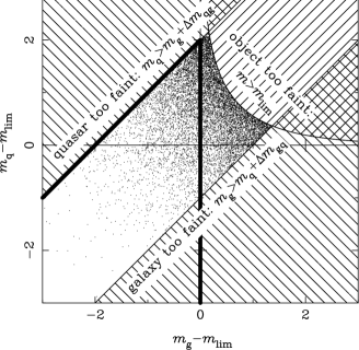
Figure 8: The range of deflector and source magnitudes ($m_{\mathrm{g}}$ and $m_{\mathrm{q}}$, respectively) probed by a GRS of magnitude limit $m_{\mathrm{l}im}$. Lenses with $-5/2\,\log(10^{-2/5\,m_{\mathrm{q}}}+10^{-2/5\,m_{\mathrm{g}}})>m_{\mathrm{l}im}$ are omitted as the combined flux from both the quasar and lens galaxy is below the flux limit. The survey is assumed to have $\Delta m_{\mathrm{q}g}=2$ (all lenses with $m_{\mathrm{q}}-m_{\mathrm{g}}>\Delta m_{\mathrm{q}g}$ being omitted as the quasar is too faint to be detectable spectroscopically) and $\Delta m_{\mathrm{g}q}=1$ (all lenses with $m_{\mathrm{g}}-m_{\mathrm{q}}>\Delta m_{\mathrm{g}q}$ being omitted as the galaxy is too faint to make the lens appear extended). Hence only those lenses which lie in the un-hatched region are included. The heavy solid lines show the boundaries of the equivalent region used by Kochanek (1992) – the inclusion of the lenses for which $m_{\mathrm{g}}>m_{\mathrm{l}im}$ is far more important than exclusion of the lenses in which the galaxy is too faint. This last point is illustrated by the scatter plot within the allowed region, which shows the distribution of galaxy-quasar pairs generated from their respective number counts [equations (12) and (20)]. For the scatter plot $m_{\mathrm{l}im}=19$ was assumed, and the quasars, being strongly lensed, are assumed to be magnified by a factor of 4 on average.

It is now possible to calculate $p_{\mathrm{q},g}$, the probability that a given galaxy (with redshift $z_{\mathrm{g}}$ and magnitude $m_{\mathrm{g}}$) lenses a given quasar [with redshift $z$, and lensed magnitude $m_{\mathrm{q}}$, defined in terms of $m$ and $m_{\mathrm{g}}$, in equation (33)]. Adjusting equation (24), the lensing probability becomes

$$p_{\mathrm{q},g}=$$ (34)

$$\frac{\theta_{\mathrm{E}}^{2}}{4}\int_{2}^{\infty}\frac{8}{\mu_{\mathrm{t}ot}^{3}}\left.\frac{{\mathrm{d}}^{2}N_{\mathrm{q}}}{{\mathrm{d}}z{\mathrm{d}}m^{\prime}}\right|_{m^{\prime}=-5/2\,\log\left(10^{-2/5\,m}-10^{-2/5\,m_{\mathrm{g}}}\right)}{\mathrm{d}}\mu_{\mathrm{t}ot},$$

if $m_{\mathrm{g},min}\leq m_{\mathrm{g}}\leq m_{\mathrm{g},max}$, but is zero if $m_{\mathrm{g}}$ is outside these limits. These, in turn, are given by

$$m_{\mathrm{g},min}=m+\frac{5}{2}\log\left(1+10^{-2/5\,\Delta m_{\mathrm{q}g}}\right)$$ (35)

and

$$m_{\mathrm{g},max}=m+\frac{5}{2}\log\left(1+10^{2/5\,\Delta m_{\mathrm{g}q}}\right).$$ (36)

The integral is along a line of constant $m$, as shown in Fig. 8. Integrating $p_{\mathrm{q},g}$ over the galaxy population yields

$$\frac{{\mathrm{d}}^{2}N_{\mathrm{l}}}{{\mathrm{d}}m{\mathrm{d}}z}=$$ (37)

$$\mbox{}\int_{0}^{\mathrm{z}_{\mathrm{q}}}\int_{m_{\mathrm{g},min}}^{m_{\mathrm{g},max}}\frac{{\mathrm{d}}V_{0}}{{\mathrm{d}}z_{\mathrm{g}}}\left.\frac{{\mathrm{d}}n_{\mathrm{g}}}{{\mathrm{d}}M}\right|_{M=M(m_{\mathrm{g}},z_{\mathrm{g}})}p_{\mathrm{q},g}\,{\mathrm{d}}m_{\mathrm{g}}\,{\mathrm{d}}z_{\mathrm{g}},$$

where the integral over the deflector magnitude is restricted again by the requirement that the overall magnitude of the lens be $m$. Finally the cumulative number counts of such lenses are

$$N_{\mathrm{l}}(<m)=\int_{-\infty}^{m}\int_{0}^{\infty}\frac{{\mathrm{d}}^{2}N_{\mathrm{l}}}{{\mathrm{d}}m{\mathrm{d}}z}\,{\mathrm{d}}z.$$ (38)

The values of $N_{\mathrm{l}}$ implied are discussed in Section 4.1, but it is immediately clear from the distribution of galaxy-quasar pairs in Fig. 8 that the majority of the lenses are included only if both the quasar and galaxy fluxes are explicitly accounted for in the calculation.

4 Results

Combining the various populations of objects considered in Section 3, it is possible to make predictions about the number of lenses found in particular redshift surveys (Section 4.1) as well as the usefulness of this search method (Sections 4.2, 4.3 and 4.4).

4.1 Number of lenses

From the number counts given in Section 3, the number of objects of type $t$ which enter a given redshift survey is

$$N_{t}=N_{\mathrm{t}ot}\frac{N_{t}(<m_{\mathrm{l}im})[1-p_{t}(<e_{\mathrm{m}in})|_{<m_{\mathrm{l}im}}]}{\sum_{t^{\prime}}N_{t^{\prime}}(<m_{\mathrm{l}im})[1-p_{t^{\prime}}(<e_{\mathrm{m}in})|_{<m_{\mathrm{l}im}}]},$$ (39)

where $N_{\mathrm{t}ot}$ is the total number of objects in the survey, $m_{\mathrm{l}im}$ the magnitude limit and $e_{\rm min}$ the ellipticity cut-off. The sum is over all the populations (i.e. $t$ = s, g, q or l, for stars, galaxies, unlensed quasars and lenses, respecitvely), although only stars and galaxies make a significant contribution to the denominator.

Fig. 9 shows the number of ‘elliptical’ lenses (and other objects) per $10^{4}$ redshifts as a function of $m_{\mathrm{l}im}$ (chosen to facilitate comparison with Kochanek 1992) for a number of different observing conditions. The lens fraction remains essentially constant at about 1 in $10^{5}$ (a) or 1 in $10^{4}$ (b), decreasing very slowly as $m_{\mathrm{l}im}$ increases, due to the decreased magnification bias. For bright surveys this is far greater than the numbers of lenses with bright deflectors considered by Kochanek (1992), but it is not at all certain that the ‘elliptical’ lenses will enter a typical GRS.

Figure 9: The expected number, $N_{t}$, of galaxies, stars, unlensed quasars and lensed quasars in a GRS as a function of the magnitude limit, $m_{\mathrm{l}im}$. The number of lenses is calculated using the spherical lens model (i.e. $\gamma_{0}=0$) in three cosmologies: $\Omega_{\mathrm{m}_{0}}=1.0$ and $\Omega_{\Lambda_{0}}=0.0$ (lower solid line); $\Omega_{\mathrm{m}_{0}}=0.3$ and $\Omega_{\Lambda_{0}}=0.0$ (middle solid line); and $\Omega_{\mathrm{m}_{0}}=0.3$ and $\Omega_{\Lambda_{0}}=0.7$ (upper solid line). The GRS is selected using an ellipticity cut $e_{\mathrm{m}in}=0.15$, and normalised to $N_{\mathrm{t}ot}=10^{4}$. The parent survey is assumed to have 3 arcsec seeing and a Moffat (1969) PSF with $\eta=2.5$ in (a) and $\eta\rightarrow\infty$ (i.e. Gaussian seeing) in (b).

Multiply-imaged quasars with lens galaxies close to the survey limit should definitely enter galaxy samples, and so they give a lower bound on $N_{\mathrm{l}}$. As can be seen from Fig. 10, these lenses are considerably rarer than the ‘elliptical’ lenses at bright magnitudes, but their numbers increase rapidly with $m_{\mathrm{l}im}$, due to the steepness of the quasar luminosity function (Section 3.3). Fig. 10 can be compared directly with the results of Kochanek (1992), although $N_{\mathrm{l}}$ is higher by a factor of $\sim 5$, due to the inclusion of the quasars’ light in the calculation. This immediately implies that the majority of any such lensed quasars found in redshift surveys should have lens galaxies which are actually fainter than the survey limit, as can be seen from Fig. 8. Other than the depth of the survey, $N_{\mathrm{l}}$ is determined mainly by $\Delta m_{\mathrm{q}g}$, with $\Delta m_{\mathrm{g}q}$ somewhat less important. The strong dependence of $N_{\mathrm{l}}$ on $\Delta m_{\mathrm{q}g}$ is again purely a function of the quasar number counts, but, being a measure of how sensitive a redshift survey is to the presence of quasar emission features, it can be determined ‘experimentally’ by running the survey software on the spectra of simulated lenses. The value of $\Delta m_{\mathrm{g}q}$ is more difficult to determine; fortunately it does not greatly affect the lens statistics, provided that $\Delta m_{\mathrm{q}g}\ga 1$. The cosmological model also has little impact on the number of lenses with visible deflectors, as the lens galaxies are so close-by that the observer-source and deflector-source distances are approximately equal (Kochanek 1992).

Figure 10: The expected number of lensed quasars, $N_{\mathrm{l}}$, per $10^{4}$ measured redshifts, shown (as in Kochanek 1992) as a function of magnitude limit, $m_{\mathrm{l}im}$. Highly elliptical sources are not included in the survey; only galaxies and lenses with $-\Delta m_{\mathrm{g}q}<m_{\mathrm{q}}-m_{\mathrm{q}}<\Delta m_{\mathrm{q}g}$ and $-5/2\log(10^{-2/5\,m_{\mathrm{q}}}+10^{-2/5\,m_{\mathrm{g}}})<m_{\mathrm{l}im}$ are included. (See Section 3.4 for a full explanation of these selection criteria.) In each panel the three sets of lines represent different values of the spectral prominence of quasars: $\Delta m_{\mathrm{q}g}=0$ (lower lines); $\Delta m_{\mathrm{q}g}=2$ (middle lines); and $\Delta m_{\mathrm{q}g}=4$ (upper lines). The morphological threshold for galaxy selection is assumed to be $\Delta m_{\mathrm{g}q}=0$ in (a) and $\Delta m_{\mathrm{g}q}=1$ in (b). For each set of observational limits, three cosmological models are shown: $\Omega_{\mathrm{m}_{0}}=1.0$ and $\Omega_{\Lambda_{0}}=0.0$ (solid lines); $\Omega_{\mathrm{m}_{0}}=0.3$ and $\Omega_{\Lambda_{0}}=0.0$ (dashed lines); and $\Omega_{\mathrm{m}_{0}}=0.3$ and $\Omega_{\Lambda_{0}}=0.7$ (dot-dashed lines).

These above results are summarised for a number of real redshift surveys in Table 1. None of the surveys have been systematically searched for lenses, although all the CfA survey spectra were examined by eye, and it was process that led to the discovery of Q 2237+0305 as a lens. If ‘elliptical’ lenses were included in the survey, the detection of a lens is not unexpected; however the CfA GRS is so bright ($\langle m\rangle\simeq 15$) that multiple point sources should have been reasonably easy to remove from the sample. Assuming only those lenses with visible, low-redshift deflectors were included, the expected number of lenses in the CfA survey is $\sim 0.03$. In other words, about 1 in 30 CfA-like galaxy samples should contain a spectroscopic quasar lens. This is considerably higher than the previous estimates of $\sim 0.0002$ (Huchra et al. 1985) and $\sim 0.003$ (Kochanek et al. 1992); the reason for this increase is simply the inclusion of the quasars’ light in the calculation. Note also that Q 2237+0305 is actually fainter than the survey limit, which is consistent with the conclusion that galaxies with $m_{\mathrm{g}}\ga m_{\mathrm{l}im}$ dominate the lens statistics.

Of the other large redshift surveys that have already been completed, both the European Southern Observatory Slice Project (ESP; Vettolani et al. 1997) and the Canadian Network for Observational Cosmology (CNOC2) sample (Yee, Ellingson & Carlberg 1996) are too small to present any real likelihood of lensing. The million galaxies in the MRSP (Schuecker et al. 1996) could include a number of lenses, although only objective prism spectra were used for the redshift determination. The selection of candidate quasars from low-grade spectra is an established technique (e.g. Hewett et al. 1995), but this would represent a considerable undertaking, as the low resolution data would generate a large number of false candidates lenses for which further observations would be required. Thus the most promising of the completed galaxy surveys is the LCRS (Shectman et al. 1996) – it is larger than the CfA survey, as well as being deeper ($\langle m\rangle\simeq 19$), and should contain one or two lenses (c.f. Fig. 10).

The two surveys listed in Table 1 which have not been completed are also the most ambitious, and are likely to yield the most lenses. The 2dF GRS (e.g. Colless 1999; Folkes et al. 1999) should contain at least 10 lenses, and as many as 50 if the cosmological model and observational parameters are optimal. Either way, it would represent the largest sample of lensed quasars generated from a single survey. However the 2dF instrument has very small optical fibres (effective radius 1 arcsec), and is unusually sensitive to a number of surface brightness-related selection effects. The impact of these on $N_{\mathrm{l}}$ is studied in more detail in Mortlock & Webster (2000c).

The SDSS (e.g. Szalay 1998; Loveday & Pier 1998) is four times the size of 2dF, and the spectra will be of considerably better quality. Assuming $\Delta m_{\mathrm{q}g}\simeq 4$ implies that $N_{\mathrm{l}}\ga 100$. Further, the survey will also include high-resolution imaging of $\sim 10^{4}{\mbox{\rm\,\,deg${}^{2}$}}$, which should allow the morphological identification of an even larger number of lens candidates. The number counts shown in Fig. 1 then imply that the SDSS should contain between 200 (if $\Omega_{\rm m_{0}}=1.0$ and $\Omega_{\Lambda_{0}}=0.0$) and 1000 (if $\Omega_{\rm m_{0}}=0.7$ and $\Omega_{\Lambda_{0}}=0.3$).

Table 1: The frequency of lensing in existing and planned GRSs.

Survey	Reference	$m_{\mathrm{l}im}$		$N_{\mathrm{t}ot}$	$N_{\mathrm{l}}$				$N_{\mathrm{l},min}$
					$\Omega_{\mathrm{m}_{0}}=1$		$\Omega_{\mathrm{m}_{0}}=0.3$		$\Omega_{\mathrm{m}_{0}}=1$
					$\Omega_{\Lambda_{0}}=0$		$\Omega_{\Lambda_{0}}=0.7$		$\Omega_{\Lambda_{0}}=0$
					$\eta=2.5$	$\eta=\infty$	$\eta=2.5$	$\eta=\infty$
CNOC2	Yee et al. (1996)	$R=21.5$	$B_{\mathrm{J}}=22.8$	$2.6\times 10^{3}$	0.01	0.03	0.08	0.2	0.3
ESP	Vettolani et al. (1997)	$B_{\mathrm{J}}=19.4$	$B_{\mathrm{J}}=19.4$	$3.3\times 10^{3}$	0.04	0.1	0.2	0.7	0.1
CfA	Geller & Huchra (1989)	$B_{\mathrm{Z}wicky}=15.5$	$B_{\mathrm{J}}=15.5$	$1.5\times 10^{4}$	0.1	0.4	0.8	2.3	0.03
LCRS	Shectman et al. (1996)	$R=17.7$	$B_{\mathrm{J}}=19.2$	$2.6\times 10^{4}$	0.3	0.8	2.3	5.7	0.9
2dF	Colless (1999)	$B_{\mathrm{J}}=19.45\!\!\!$	$B_{\mathrm{J}}=19.45\!\!\!$	$2.5\times 10^{5}$	2.5	7.5	18	50	10
MRSP	Schuecker et al. (1996)	$J=20$	$B_{\mathrm{J}}=19.5$	$9.0\times 10^{5}$	4.5	18	36	90	27
SDSS	Szalay (1998)	$r_{\mathrm{G}unn}=18.2$	$B_{\mathrm{J}}=18.9$	$1.0\times 10^{6}$	10	40	90	250	100

A summary of the number of lenses expected in several completed and future redshift surveys. For each survey: $m_{\mathrm{l}im}$ is the magnitude limit in the band indicated (with approximate conversions to $B_{\mathrm{J}}$, based on the redshift coverage of the survey); $N_{\mathrm{t}ot}$ is the total number of redshifts measured; $N_{\mathrm{l}}$ is the expected number of lenses; and $N_{\mathrm{l},min}$ is the expected number of lenses if only those with visible detectors are included in the survey. The variation of $N_{\mathrm{l}}$ with cosmological model and PSF is given explicitly, but the spherical lens model and 3 arcsec seeing are assumed. On the other hand, $N_{\mathrm{l},min}$ is strongly dependent on neither the cosmology, nor the PSF in the relevant magnitude range, and so is only shown for the Einstein-de Sitter model. In all cases $N_{\mathrm{l},min}$ is calculated assuming $\Delta m_{\mathrm{g}q}=0$ and $\Delta m_{\mathrm{q}g}=2$, except for the MRSP (which uses objective prism spectra, and so has $\Delta m_{\mathrm{q}g}\simeq 0$) and the SDSS (which will obtain high-quality spectra with $\Delta m_{\mathrm{q}g}\simeq 4$).

4.2 Control samples

Kochanek (1992) suggested two control samples – foreground stars and unlensed quasars – from which the efficiency and completeness of the lens search could be calibrated. However these objects are only useful controls if they enter the GRS mainly through chance superpositions with survey galaxies. Unfortunately, most of the stars and unlensed quasars in the survey are not there due to chance alignments, but misclassification (e.g. Fig. 9). For instance, the limitations APM star-galaxy separation algorithm (e.g. Maddox et al. 1990a) imply that, of the $\sim 2.5\times 10^{5}$ objects in the 2dF GRS, several thousand will be stars, compared to only several tens of star-galaxy superpositions. With the exception of the brightest surveys ($m_{\mathrm{l}im}\la 18$), the same is also true for unlensed quasars.

This effectively leaves this lens search technique without any simple calibration, which is not important if the aim is simply to discover new lenses, but must be addressed if lensing probabilities are to be determined. One possibility is to perform both morphological and spectroscopic calibration a posteriori by simulating quasar-galaxy lenses and analysing them using the software actually used for the survey. This also has the advantage of taking into account all of the potential biases in the survey without the need for explicit modelling.

4.3 Efficiency and completeness

The sheer number of quasars that must be re-imaged per lens discovery in a conventional lens survey is prohibitive (e.g. Section 1), and it is one of the major reasons that so few lenses are known. The use of morphological selection, implicit in a GRS, can increase the efficiency by removing most of the unlensed quasars from the survey, but there is also a significant reduction in the completeness of the lens sample.

The completeness is simply $C=1-p_{\mathrm{l}}(<e_{\mathrm{m}in})|_{<m_{\mathrm{l}im}}$, where $e_{\mathrm{m}in}$ is the ellipticity cut of the survey and $m_{\mathrm{l}im}$ its magnitude limit. As shown in Fig. 7, this is quite variable, with $C$ ranging between $0.05$ and $0.5$, depending mainly on the form of the PSF. However a low value of $C$ is not necessarily a problem, provided that its value is reasonably well known. Note that $C$ is unambiguously defined only for the ‘elliptical’ lens sample; the lenses with $m_{\mathrm{g}}\simeq{\mbox{\rm\,\,m}}_{\mathrm{q}}$ are not drawn from a well-defined parent population.

More important is the efficiency, $E$, which is defined as the number of high-resolution re-observations required per lens discovery. For a redshift survey-based lens search it is [c.f. equation (16)]

$$E_{\mathrm{GRS}}=\frac{N_{\mathrm{l}}(<m_{\mathrm{l}im})p_{\mathrm{l}}(<e_{\mathrm{m}in})\,|_{<m_{\mathrm{l}im}}}{N_{\mathrm{q}}(<m_{\mathrm{l}im})p_{\mathrm{q}}(<e_{\mathrm{m}in})\,|_{<m_{\mathrm{l}im}}},$$ (40)

as only those objects with quasar-like spectra need to be re-imaged. As shown in Fig. 11, this is generally much higher than the efficiency of a conventional lens survey,

$$E_{\mathrm{l}ens\,survey}=\frac{N_{\mathrm{l}}(<m_{\mathrm{l}im})}{N_{\mathrm{q}}(<m_{\mathrm{l}im})},$$ (41)

where it is optimisticly assumed that the lens sample is essentially complete. For bright surveys $E_{\mathrm{GRS}}\simeq 1$ as the star-galaxy separation techniques are so reliable, although close quasar-galaxy associations have not been included. For fainter magnitude limits $E$ decreases for both search methods, due to the lower lensing fraction, and for $m_{\mathrm{l}im}\ga 20$ the efficiency of redshift surveys approaches that of lens surveys.

If only lenses with bright deflectors enter a galaxy survey, then $E_{\mathrm{GRS}}$ is reduced by about an order of magnitude, but is still greater than $E_{\mathrm{l}ens\,survey}$ for $m_{\mathrm{l}im}\la 20$. Hence the efficiency of lens searches based on GRS spectra is almost always greater than that of conventional lens surveys.

Figure 11: The detection efficiency of a conventional lens survey, $E_{\mathrm{l}ens\,survey}$ (lower lines), and that of a lens search based on a redshift survey, $E_{\mathrm{GRS}}$ (upper lines), as a function of the limiting magnitude of the survey, $m_{\mathrm{l}im}$. Both are defined in Section 4.3, and $E_{\mathrm{GRS}}$ is shown for two values of $\eta$ used in the definition of the Moffat (1969) PSF: $\eta=2.5$ and $\eta\rightarrow\infty$ (Gaussian seeing), as labelled. In each case three cosmological models are used: $\Omega_{\rm m_{0}}=1.0$ and $\Omega_{\Lambda_{0}}=0.0$ (solid lines); $\Omega_{\rm m_{0}}=0.3$ and $\Omega_{\Lambda_{0}}=0.0$ (dashed lines); and $\Omega_{\rm m_{0}}=0.3$ and $\Omega_{\Lambda_{0}}=0.7$ (dot-dashed lines).

4.4 Deflector redshift distribution

By evaluating the lensing probability (Section 3.4) for a fixed deflector redshift, the distribution of lens galaxy redshifts, ${\mathrm{d}}p/{\mathrm{d}}z_{\mathrm{g}}$, can be found; this is shown in Fig. 12. The ‘elliptical’ lenses have the broad range of deflector redshifts expected of a conventional lens survey (e.g. Turner et al. 1984), and, in particular, the expected number of nearby deflectors is very small. The distribution is very different if only lenses with visible lens galaxies are selected – it roughly matches the overall redshift distribution of a GRS with a limiting magnitude of $m_{\mathrm{l}im}+\Delta m_{\mathrm{q}g}$ (c.f. Fig. 4). Hence the 2dF redshift survey should yield one or two lenses with $z_{\mathrm{g}}\la 0.1$, and the SDSS could contain about ten lenses with such nearby deflectors.

Figure 12: The normalised distribution of deflector redshifts, $z_{\mathrm{g}}$, of lensed quasars discovered in GRSs. For the ‘elliptical’ lenses (broader curves) the distribution is determined solely by the cosmological model, whereas the extent of the distribution for the lenses with bright deflectors increases with the depth of the survey. The two sets of curves for each type of lens show the distributions with $m_{\mathrm{l}im}=18$ and $m_{\mathrm{l}im}=20$. For each survey $\Delta m_{\mathrm{q}g}=2$, and results are presented for three cosmological models: $\Omega_{\rm m_{0}}=1.0$ and $\Omega_{\Lambda_{0}}=0.0$ (solid lines); $\Omega_{\rm m_{0}}=0.3$ and $\Omega_{\Lambda_{0}}=0.0$ (dashed lines); and $\Omega_{\rm m_{0}}=0.3$ and $\Omega_{\Lambda_{0}}=0.7$ (dot-dashed lines).

5 Conclusions

Due to the imperfect discrimination between galaxies and other celestial objects, gravitationally-lensed quasars enter GRS catalogues, and should then be detectable spectroscopically. The gravitational lens Q 2237+0305 was discovered in this way (Huchra et al. 1985), and Kochanek (1992) predicted approximately one lens per $10^{6}$ redshifts measured. However the inclusion of the quasars’ light in the calculation of the lens galaxies’ magnitudes increases the number of lenses by up to an order of magnitude, as illustrated in Fig. 8. Another possibility is that many lensed quasars enter GRSs as the quasar images combine to have a high ellipticity, but are also unresolved in the low-resolution (e.g. plate) data from which candidate galaxies are selected. If a significant fraction of such lenses are observed spectroscopically in GRSs, more new lenses will be discovered in redshift surveys than are known to date.

The number of lenses expected in various existing and planned surveys is given in Table 1. It can be seen that $N_{\mathrm{l}}$ varies greatly with both the form of the PSF of the parent survey and the cosmological model (in the case of the ‘elliptical’ lenses), which places fundamental limits on the accuracy of these predictions. For instance, the current generation of surveys (with up to $\sim 2\times 10^{4}$ galaxies) should contain several lenses between them, but the above uncertainties, combined with shot noise, make this a rather weak prediction. Looking ahead, the 2dF GRS (with $\sim 2.5\times 10^{5}$ galaxies to a limit of $m_{B_{\mathrm{J}}}=19.5$) is already well underway, and should contain at least 10 new lenses, and up to 50 if observational conditions are favourable. Howver, it is particularly sensitive to surface brightness-related selection effects, and a more detailed simulation of lensing in the 2dF redshift survey is presented in Mortlock & Webster (2000c). Finally, the SDSS can be expected to contain over 100 spectroscopic lensed quasars, along with even more discovered by more conventional methods.

Many, and possibly all, of the lenses discovered spectroscopically in redshift surveys, will have deflector galaxies at low redshifts, comparable to the depth of the survey proper. These have the potential to be the most important products of such a lens search, as the proximity of the deflector, combined with the information provided by the lensing event, can provide a number of unique insights, as exemplified by Q 2237+0305. The 2dF GRS should contain several low-redshift lenses, and the SDSS about 10. Of course not all of these will have Q 2237+0305’s wonderful combination of source and deflector properties, but the possibility of even one similar system is tantalising, to say the least.

References

- [Bahcall & Soneira 1980] Bahcall J. N., Soneira R. M., 1980, ApJS, 44, 73
- [Barnes et al. 1999] Barnes D. G., Webster R. L., Schmidt R. W., Hughes A., 1999, MNRAS, 309, 641
- [Baugh & Efstathiou 1993] Baugh C. M., Efstathiou G., 1993, MNRAS, 265, 145
- [Binney & Tremaine 1987] Binney J. J., Tremaine S., 1987, Galactic Dynamics. Princeton University Press, Princeton
- [Boyle et al. 1999a] Boyle B. J., Croom S. M., Smith R. J., Shanks T., Miller L., Loaring N. S., 1999a, Phil. Trans. of the Royal Soc. A, 357, 185
- [Boyle et al. 1999b] Boyle B. J., Croom S. M., Smith R. J., Shanks T., Miller L., Loaring N. S., 1999b, in Morganti R., Couch W. J., eds, Looking Deep in the Southern Sky. Springer-Verlag, Berlin, p. 16
- [Boyle et al. 1988] Boyle B. J., Shanks T., Peterson B. A., 1988, MNRAS, 235, 935
- [Brainerd et al. 1996] Brainerd T. G., Blandford R. D., Smail I. S., 1996, ApJ, 466, 623
- [Burke et al. 1992] Burke B. F., Lehár J., Connor S. R., 1992, in Kayser R., Schramm T., Nieser L., eds, Gravitational Lenses. Springer-Verlag, Berlin, p. 237
- [Carroll et al. 1992] Carroll S. M., Press W. H., Turner E. L., 1992, ARA&A, 30, 499
- [Chae et al. 1998] Chae K.-H., Turnshek D. A., Khersonsky V. K., 1998, ApJ, 495, 609
- [Chen et al. 1995] Chen G. H., Kochanek C. S., Hewitt J. N., 1995, ApJ, 447, 62
- [Colless 1999] Colless M. M., 1999, in Morganti R., Couch W. J., eds, Looking Deep in the Southern Sky. Springer-Verlag, Berlin, p. 9
- [Crampton et al. 1992] Crampton D., McClure R. D. & Fletcher J. M., 1992, ApJ, 392, 23
- [de Vaucouleurs & Olson 1982] de Vaucouleurs G., Olson D. W., 1982, ApJ, 256, 346
- [Drinkwater et al. 1999] Drinkwater M. J., Phillipps S., Gregg M. D., Parker Q. A., Smith R. M., Davies J. I., Jones J. B., Sadler E. M., 1999, ApJ, 511, L97
- [Efstathiou et al. 1988] Efstathiou G., Ellis R. S., Peterson B. A., 1988, MNRAS, 232, 431
- [Faber & Jackson 1976] Faber S. M., Jackson R. E., 1976, ApJ, 204, 668
- [Falco 1993] Falco E. E., 1993, in Surdej J., Fraipont-Caro D., Gosset E., Refsdal S., Remy M., eds, Proc. 31st Liège Int. Astroph. Coll., Gravitational Lenses in the Universe. Université de Liège, Liège, p. 127
- [Falco et al. 1999] Falco E. E. et al., 1999, ApJ, 523, 617
- [Fisher et al. 1995] Fisher K. B., Huchra J. P., Strauss M. A., Davis M., Yahil A., Schlegel D., 1995, ApJS, 100, 69
- [Folkes et al. 1999] Folkes S. R. et al., 1999, MNRAS, 308, 459
- [Foltz et al. 1992] Foltz C. B., Hewett P. C., Webster R. L., Lewis G. F., 1992, ApJ, 386, L43
- [Geller & Huchra 1989] Geller M. J., Huchra J. P., 1989, Science, 246, 897
- [Godwin et al. 1983] Godwin J. G., Metcalfe N., Peach J. V., 1983, MNRAS, 202, 113
- [Grogin & Narayan 1996] Grogin N. A., Narayan R., 1996, ApJ, 464, 92
- [Hartwick & Schade 1990] Hartwick F. D. A., Schade D., 1990, ARA&A, 28, 437
- [Hewett et al. 1995] Hewett P. C., Foltz C. B., Chaffee F. H., 1995, AJ, 109, 1498
- [Hewitt & Burbidge 1993] Hewitt J. N., Burbidge G., 1993, ApJS, 87, 2
- [Huchra et al. 1985] Huchra J. P., Gorenstien M., Kent S., Shapiro I., Smith G., Horine E., Perley R., 1985, AJ, 90, 691
- [Jackson et al. 1995] Jackson N. et al., 1995, MNRAS, 274, L25
- [Jarvis & Tyson 1981] Jarvis J. F., Tyson J. A., 1981, AJ, 86, 476
- [Jaunsen et al. 1995] Jaunsen A. O., Jablonski M., Petterson B. R., Stabell R., 1995, A&A, 300, 323
- [Jones et al. 1991] Jones L. R., Fong R., Shanks T., Ellis R. S., Peterson B. A., 1991, MNRAS, 249, 481
- [Keeton & Kochanek 1996] Keeton C., Kochanek C. S., 1996, in Kochanek C. S., Hewitt J. N., eds, Proc. IAU Symp. No. 173. Astrophysical Applications of Gravitational Lensing. Kluwer, Dordrecht, p. 419
- [Keeton & Kochanek 1998] Keeton C., Kochanek C. S., Falco E. E., 1998, ApJ, 509, 561
- [Kent & Falco 1988] Kent S. M., Falco E. E., 1988, AJ, 96, 1570
- [King 1971] King I. R., 1971, PASP, 88, 199
- [Kinney et al. 1996] Kinney A. L., Calzetti D., Bohlin R. C., McQuade K., Storchi-Bergmann T., Schmitt H. R., 1996, ApJ, 467, 38
- [Kochanek 1991] Kochanek C. S., 1991, ApJ, 379, 517
- [Kochanek 1992] Kochanek C. S., 1992, ApJ, 397, 381
- [Kochanek 1993a] Kochanek C. S., 1993a, ApJ, 419, 12
- [Kochanek 1993b] Kochanek C. S., 1993b, MNRAS, 261, 453
- [Kochanek 1994] Kochanek C. S., 1994, ApJ, 436, 56
- [Kochanek 1995] Kochanek C. S., 1995, ApJ, 453, 545
- [Kochanek 1996a] Kochanek C. S., 1996a, ApJ, 466, 638
- [Kochanek 1996b] Kochanek C. S., 1996b, ApJ, 473, 595
- [Kochanek et al. 1995] Kochanek C. S., Falco E. E., Schild R., 1995, ApJ, 452, 109
- [Kovner 1987] Kovner I., 1987, ApJ, 312, 22
- [Kundić et al. 1997] Kundić, T. et al., 1997, ApJ, 482, 75
- [Lehár et al. 1993] Lehár J., Langston G. I., Silber A. D., Lawrence C. R., Burke B. F., 1993, AJ, 105, 847
- [Lehár et al. 1996] Lehár J., Cooke A. J., Lawrence C. R., Silber A. D., Langston G. I., 1996, AJ, 111, 1812
- [Lewis & Irwin 1996] Lewis G. F., Irwin M. J., 1996, MNRAS, 283, 225
- [Loveday & Pier 1998] Loveday J., Pier J., 1998, in Colombi S., Mellier Y., Raban B., eds, Wide Field Surveys in Cosmology. Edition Frontiers, Paris, p. 317
- [Maddox et al. 1990a] Maddox S. J., Efstathiou G., Sutherland W. J., Loveday J., 1990a, MNRAS, 243, 692
- [Maddox et al. 1990b] Maddox S. J., Sutherland W. J., Efstathiou G., Loveday J., Peterson B. A., 1990b, MNRAS, 247, 1P
- [Malhotra et al. 1996] Malhotra S., Rhoads J. E., Turner E. L., 1997, MNRAS, 288, 138
- [Maoz et al. 1993a] Maoz D., Bahcall J. N., Doxsey R., Schneider D. P., Bahcall N. A., Lahav O., Yanny B., 1993a, ApJ, 402, 69
- [Maoz et al. 1993b] Maoz D. et al., 1993b, ApJ, 409, 28
- [Maoz et al. 1992] Maoz D. et al., 1992, ApJ, 386, L1
- [Moffat 1969] Moffat A. F. J., 1969, A&A, 3, 455
- [Mortlock 1999] Mortlock D. J., 1999, PhD Thesis, University of Melbourne
- [Mortlock & Webster 2000a] Mortlock D. J., Webster R. L., 2000a, MNRAS, in press
- [Mortlock & Webster 2000b] Mortlock D. J., Webster R. L., 2000b, MNRAS, in press
- [Mortlock & Webster 2000c] Mortlock D. J., Webster R. L., 2000c, MNRAS, submitted
- [Myers et al. 1995] Myers S. T., et al., 1995, ApJ, 447, L5
- [Patnaik et al. 1992] Patnaik A. R., Browne I. W. A., Wilkinson P. N., Wrobel J. M., 1992, MNRAS, 254, 655
- [Peterson 1997] Peterson B. M., 1997, An Introduction to Active Galactic Nuclei, Cambridge University Press, Cambridge
- [Postman & Geller 1984] Postman M., Geller M. J., 1984, ApJ, 281, 95
- [Rauch & Blandford 1992] Rauch K. P., Blandford R. D., 1992, ApJ, 381, L39
- [Refsdal 1964] Refsdal S., 1964, MNRAS, 128, 307
- [Saglia et al. 1993] Saglia R. P., Bertschinger E., Baggley G., Burstein D., Colless M. M., Davies R. L., McMahan R. K., Wegner G., 1993 MNRAS, 264, 961
- [Saunders et al. 1998] Saunders W., et al., 1998 in Colombi S., Mellier Y., Raban B., eds, Wide Field Surveys in Cosmology. Edition Frontiers, Paris, p. 71
- [Schechter 1976] Schechter P., 1976, ApJ, 203, 297
- [Schmidt & Wambsganss 1998] Schmidt R. W., Wambsganss J., 1998, A&A, 335, 379
- [Schmidt et al. 1998] Schmidt R. W., Webster R. L., Lewis G. F., 1998, MNRAS, 295, 488
- [Schneider et al. 1992] Schneider P., Ehlers J., Falco E. E., 1992, Gravitational Lenses, Springer-Verlag, Berlin
- [Schuecker 1996] Schuecker P., Ott H.-A., Seitter W. C., 1996, ApJ, 459, 467
- [Shectman et al. 1996] Shectman S. A., Landy S. D., Oemler A., Tucker D. L., Kirshner R. P., Lin H., Schechter P. L., 1996, ApJ, 470, 172
- [Stobie & Ishida 1987] Stobie R. S., Ishida K., 1987, AJ, 93, 624
- [Surdej et al. 1993] Surdej J., et al., 1993, AJ, 205, 2064
- [Szalay 1998] Szalay A. S., 1998, in Müller V., Gottlöber S., Mücket J. P., Wambsganss J., eds, Large Scale Structure: Tracks and Traces. World Scientific, Singapore, p. 97
- [Tody 1986] Tody D., 1986, Proceedings of Society of Photo-Optical Instrument Engineers, 627, 733
- [Tully & Fisher 1977] Tully R. B., Fisher J. R., 1977, A&A, 54, 661
- [Turner 1980] Turner E. L., 1980, ApJ, 242, L135
- [Turner 1990] Turner E. L., 1990, ApJ, 365, L43
- [Turner et al. 1984] Turner E. L., Ostriker J. P., Gott J. R., 1984, ApJ, 284, 1
- [Vettolani et al. 1997] Vettolani G., et al., 1997, A&A, 325, 954
- [Wambsganss et al. 1990] Wambsganss J., Paczyński B., Schneider P., 1990, ApJ, 358, L33
- [Warren et al. 1991] Warren S. J., Hewett P. C., Osmer P. S., 1991, ApJ, 76, 23
- [Webster et al. 1988] Webster R. L., Hewett P. C., Irwin M. J., 1988, AJ, 95, 19
- [Wyithe et al. 1999] Wyithe J. S. B., Webster R. L., Turner E. L., 1999, MNRAS, 309, 261
- [Wyithe et al. 2000a] Wyithe J. S. B., Webster R. L., Turner E. L., 2000a, MNRAS, 312, 843
- [Wyithe et al. 2000b] Wyithe J. S. B., Webster R. L., Turner, E. L., 2000b, MNRAS, 315, 51
- [Wyithe et al. 2000c] Wyithe J. S. B., Webster R. L., Turner E. L., Mortlock D. J., 2000c, MNRAS, 315, 62
- [Yee 1988] Yee H. K. C., 1988, AJ, 95, 1331
- [Yee et al. 1996] Yee H. K. C., Ellingson E., Carlberg R. G., 1996, ApJS, 102, 269
- [Yee et al. 1993] Yee H. K. C., Filippenko A. V., Tang D., 1993, AJ, 105, 7