SUPERNOVA REMNANTS IN THE SEDOV EXPANSION PHASE: THERMAL X-RAY EMISSION

Abstract

Improved calculations of X-ray spectra for supernova remnants (SNRs) in the Sedov-Taylor phase are reported, which for the first time include reliable atomic data for Fe L-shell lines. This new set of Sedov models also allows for a partial collisionless heating of electrons at the blast wave and for energy transfer from ions to electrons through Coulomb collisions. X-ray emission calculations are based on the updated Hamilton-Sarazin spectral model. The calculated X-ray spectra are succesfully interpreted in terms of three distribution functions: the electron temperature and ionization timescale distributions, and the ionization timescale averaged electron temperature distribution. The comparison of Sedov models with a frequently used single nonequilibrium ionization (NEI) timescale model reveals that this simple model is generally not an appropriate approximation to X-ray spectra of SNRs. We find instead that plane-parallel shocks provide a useful approximation to X-ray spectra of SNRs, particularly for young SNRs. Sedov X-ray models described here, together with simpler plane shock and single ionization timescale models, have been implemented as standard models in the widely used XSPEC v11 spectral software package.

1 INTRODUCTION

X-ray astronomy has advanced significantly in recent years because of improved X-ray instrumentation. Several recent X-ray satellites provided complementary capabilities: high spatial resolution and mapping of the entire sky (ROSAT), spatially-resolved spectroscopy (ASCA), and broad-band coverage (BeppoSAX). In the field of supernova remnants (SNRs), this has led to many advances, such as the discovery of the nonthermal synchrotron X-ray emission produced by energetic electrons accelerated at a shock front, identification of a number of new neutron stars and associated synchrotron nebulae, discovery of new SNRs, and identification of young, ejecta-dominated SNRs. Spatially-resolved X-ray spectroscopy, provided by the ASCA satellite, played a crucial role in these discoveries. The ASCA database now contains a large number of excellent spectra of SNRs. Observations with the next generation of X-ray satellites (Chandra and XMM-Newton) have begun to provide even better quality data, ensuring continuing progress in the SNR research.

While the new X-ray observations led to significant progress, X-ray spectral data on SNRs, and ASCA data in particular, have been mostly underutilized. The fundamental reason for this unsatisfactory situation is that X-ray emitting plasmas in SNRs are not in ionization equilibrium, significantly complicating analysis of their X-ray spectra. Until recently most X-ray observers have not had access even to simple nonequilibrium ionization (NEI) models. The simplest NEI model consists of an impulsively heated, uniform and homogeneous gas, initially cold and neutral. While this constant temperature, single-ionization timescale model is often used in analysis of X-ray spectra of SNRs, in most cases it is unlikely to be a good approximation to shock-heated plasmas in SNRs. Because X-ray spectra are sensitive to the detailed structure of a SNR, the best description of SNR spectra is through hydrodynamical modeling, coupled with X-ray emission calculations. This approach is obviously impractical in most cases. That leaves idealized hydrodynamical structures, such as self-similar hydrodynamical solutions, as the best choice for general NEI models. The Sedov-Taylor self-similar solution, describing a point blast explosion in a uniform ambient medium, is the most well-known and useful of such structures.

X-ray emission calculations for the Sedov models have been performed numerous times in the past, with the most extensive set of calculations presented by Hamilton, Sarazin, & Chevalier (1983). The shape of the X-ray spectrum, spatially integrated over the whole remnant, depends on the shock speed $v_{s}$, the ionization timescale $\tau_{0}$ (which we define as the product of the remnant’s age $t_{0}$ and the postshock electron number density $n_{es}$), and the extent of electron heating at the shock front. In addition, as typical for most X-ray emitting thermal plasmas, line strengths and to a lesser extent continua depend on heavy-element abundances. Sedov models have been recalculated using updated atomic data (Kaastra & Jansen 1993) and successfully applied to modeling of X-ray spectra of SNRs in the Large Magellanic Cloud (Hughes, Hayashi, & Koyama 1998).

The most uncertain aspect of X-ray modeling in the framework of the Sedov model is the extent of electron heating in a blast wave. Because of the low densities typical for the interstellar medium (ISM), shocks in the ISM are collisionless, where the ordered ion kinetic energy is dissipated into random thermal motions through collisionless interactions involving magnetic fields. Electrons, whose collisions with ions produce the observed X-ray emission from SNRs, are most likely also heated to some degree in collisionless shocks, but the details of this process are not well understood. In the extreme case of a very high Mach-number shock, in the shock frame both electrons and ions enter with the shock velocity $v_{s}$, so that after randomization one expects $kT_{i}\sim m_{i}v_{s}^{2}$ and $kT_{e}\sim m_{e}v_{s}^{2}$, that is, $T_{e}/T_{i}\sim 1/1836$, unless some collisionless heating of electrons (at the expense of ions) also occurs. Hamilton et al. (1983) considered two extreme possibilities, either full electron–ion equilibration at the shock front, or electron heating only through Coulomb collisions in the postshock gas, without any collisionless heating at the front itself. Hughes et al. (1998) used these two limiting classes of models in their modeling of LMC SNRs, and found better (but not perfect) agreement for models without any collisionless heating. While these results suggest that the full electron–ion equipartition might not hold in SNRs, the extent of collisionless electron heating remains an open question.

These questions are critical for observations since both the X-ray continuum and lines originate from electrons: from electron bremsstrahlung or electron impact excitation of ions. Until X-ray observations are able to resolve thermal Doppler widths of emission lines, ion energy remains invisible except as a pool from which to heat electrons. The detailed shape of the electron distribution affects both continuum and line emission. This introduces another potential problem: the possible deviation of the electron energy distribution function from a Maxwellian distribution, in particular the presence of a high-energy tail. Electrons in such a tail might modify the high-energy X-ray spectrum of a SNR through interactions with ions and magnetic fields.

Theoretical modeling of collisionless shocks, performed with the purpose of accounting for the observed intensity and properties of Galactic cosmic rays, revealed that energetic particles generated within the shock should strongly modify the shock structure. Such cosmic-ray modified shocks transfer a significant amount of kinetic energy into cosmic rays, which then diffuse upstream of the original shock and partially decelerate incoming gas in a region ahead of it (the shock precursor). The temperature of the thermal gas is much lower than in a standard (nonmodified) shock with the same velocity, because of this efficient transfer of kinetic energy into cosmic rays. This will affect X-rays produced by thermal plasmas in cosmic-ray modified shocks, because of strong dependence of X-ray emission on gas temperature. The modeling of modified shocks has been usually done in the framework of steady-state, plane-parallel shocks, preventing a direct comparison with the Sedov model discussed above. Such a comparison is now possible, as time-dependent, cosmic-ray modified shock models have been constructed recently by Berezhko, Yelshin, & Ksenofontov (1994, 1996).

The continuing improvement in theory just described is not followed by a similar improvement in the X-ray data analysis. Instead of using Sedov models (and even more sophisticated hydrodynamical models, including those with cosmic-ray modified shocks), many observers still rely on the ionization equilibrium models, which are generally not acceptable for SNRs. Sometimes spectra are modeled by Gaussian lines and free-free continua, a purely phenomenological approach which does not allow for determination of physical parameters in X-ray emitting plasma. The frequently used constant temperature, single ionization timescale NEI model is better than an equilibrium plasma model, but it is still not appropriate for SNRs. In order to make full advantage of current and future X-ray data on SNRs. a concentrated effort is required to close the gap between the relatively sophisticated theory and the current crude data analysis. The theoretical work described here focuses on a most basic set of models which is necessary for analysis of X-ray data, and which should be routinely used by X-ray observers. We present new calculations of spatially-integrated X-ray emission from Sedov models in § 2, allowing for partial electron heating at a shock front. A preliminary version of this work was presented in Lyerly et al. (1997). In § 3, we discuss our results in terms of suitably chosen temperature and ionization timescale distribution functions, and compare Sedov models with simpler NEI models such as a single timescale, constant temperature model or a plane-parallel shock. The sensitivity of X-ray spectra to model parameters is discussed in § 4. We present a summary of our results in § 5.

2 X-RAY EMISSION CALCULATIONS

2.1 Sedov-Taylor Dynamics

We base our spectral calculations on a Sedov-Taylor (ST) blast wave model. The ST model begins with a spherically symmetric point blast expanding adiabatically into a uniform ambient medium with the adiabatic index $\gamma=5/3$. Only the shocked ISM is considered in the ST model. Therefore, the shocked ISM mass must significantly outweigh the mass of the material ejected by the supernova (SN), usually at an age of a few thousand years. The governing parameters of this phase of SNR evolution are the initial energy of the blast $E$, the density of the ambient medium $\rho_{0}$, and the time since the explosion $t_{0}$. These parameters can be easily arranged to form a unit of length, related to the shock radius by $r_{s}=1.15\left(Et_{0}^{2}/\rho_{0}\right)^{1/5}$. These three initial parameters completely determine the dynamics of a Sedov model. For example, we might choose an initial energy of $10^{51}$ ergs, an upstream hydrogen number density $n_{0}=1$ cm^-3, and a time $t_{0}$ of $10^{11}$ seconds, yielding a radius of $2.5\times 10^{19}$ cm. We now know the shock speed, $v_{s}=0.4r_{s}/t_{0}$, and also the postshock values of pressure, density, and velocity through the Rankine-Hugoniot shock conditions. The self-similar analytical solution (Sedov 1946; Taylor 1950) gives the pressure, density and velocity profiles behind the shock, and it allows us to find pressure and density variations as a function of time for each fluid element. This information is necessary for determination of the ionization state for each ion species.

Hamilton et al. (1983) showed that the shape of the X-ray spectrum of a spatially-integrated Sedov model does not depend on all three parameters mentioned above, but only on shock velocity $v_{s}$ (or alternatively shock temperature $T_{s}=1.37\times 10^{7}(v_{s}/1000\mbox{ km s}^{-1})^{2}~{}{\rm K}=1.18(v_{s}/1000\mbox{ km s}^{-1})^{2}$ keV) and parameter $\eta=n_{0}^{2}E$. (We have assumed cosmic-abundance plasma, where electrons are provided by fully ionized H and He, with a negligible contribution from heavier elements. The mean mass per particle $\mu$ is then equal to 0.6 in units of $m_{p}$.) In order to simplify comparison with other NEI models, we use ionization timescale $\tau_{0}$ instead of $\eta$, where we define $\tau_{0}$ as the product of the postshock electron density $n_{es}$ and the remnant’s age $t_{0}$. Note that for cosmic-abundance plasma and the strong shock Rankine-Hugoniot jump conditions, $n_{es}=4.8n_{0}$. From equation (4b) in Hamilton et al. (1983), ionization timescale $\tau_{0}$ is equal to $6.03\times 10^{11}\eta_{51}^{1/3}T_{7}^{-5/6}$ cm^-3 s, where $\eta_{51}=\eta/10^{51}$ ergs cm^-6 and $T_{7}=T_{s}/10^{7}$ K. X-ray spectra depend also on electron temperature $T_{e}$ which is discussed next.

Figure 1: Electron temperature $T_{e}$ vs emission measure $EM$ (both normalized to 1 at the shock), for Sedov model with $T_{s}=3\times 10^{7}$ K, $\tau_{0}=5\times 10^{11}$ cm^-3 s, and with full ion-electron equipartition ($T_{e}=T$; solid curve), no collisionless heating of electron at the shock (dotted curve), and partial electron heating at the shock with the postshock electron temperature $T_{es}=0.5T_{s}=1.5\times 10^{7}$ K (dashed curve).

Figure 2: Ratio of electron temperature $T_{e}$ to the mean gas temperature $T$ vs emission measure $EM$, for the Sedov model with the same $T_{s}$ and $\tau_{0}$ as in Figure 1, but with various amounts of collisionless heating ($\beta$ ranges from 0.0 at the bottom to 0.9 at the top).

2.2 Electron Temperature

The mean gas temperature $T$ in Sedov models is plotted in Figure 1 as a function of the normalized emission measure $EM(r)=\int_{0}^{r}n_{e}n_{p}dr/\int_{0}^{r_{s}}n_{e}n_{p}dr$. (Because we assumed normal abundances, with a cosmic H/He ratio and a negligible contribution to electron density from elements heavier than He, models and calculations discussed in this work are not applicable to heavy-element plasmas where these assumptions break down.) $T$ is equal to the shock temperature $T_{s}$ at the shock ($EM=1$), and increases toward the remnant’s interior. But for calculations of X-ray spectra we need to know the electron temperature $T_{e}$, which in general is not equal to either the mean temperature $T$ or the ion temperature $T_{i}$. These three temperature are equal only if electrons and ions are equilibrated at the shock front through plasma instabilities generated within the collisionless plasma. Because kinetic energy is initially transferred to thermal motions of ions in collisionless shocks, full equilibration demands the presence of a very efficient mechanism for transfer of energy from ions to electrons in collisionless shocks, at all shock Mach numbers. This is unlikely based on available observational and theoretical evidence. For example, observations of ultaviolet (UV) lines from a fast nonradiative shock in SN 1006 (Laming et al. 1996) suggest that there is little energy transfer from ions to electrons in shocks where neutral H is present ahead of the shock front. In an extreme case of a very inefficient heating of electrons at the shock, the postshock electron temperature $T_{es}$ is much less than the postshock ion temperature $T_{is}$, and the ratio $T_{es}/T_{is}$ (or $T_{es}/T_{s}$) is close to 0. Electrons are then heated mostly in Coulomb collisions with ions in the hot shocked plasma downstream of the shock front. The most general situation, most likely to happen in SNRs shocks, is that electrons are partially heated in collisionless shocks and additional Coulomb heating occurs downstream of the shock.

The extent of electron heating in shocks can be parametrized by the temperature ratio $\beta\equiv T_{es}/T_{s}$, which can vary from nearly $0$ in shocks with negligible collisionless heating to $1$ when this heating is very efficient. In general, $\beta$ might depend on the shock Mach number and other shock parameters, possibly decreasing with increasing shock Mach number (Bykov & Uvarov 1999). This inverse correlation with the shock Mach number is supported by most recent observational evidence based on optical observations of nonradiative shocks (Ghavamian 1999; Ghavamian et al. 2000). Because of the poor understanding of electron heating in collisionless shocks, which may depend not only on the shock Mach number but also on other shock parameters such as the magnetic field orientation, we neglect dependence of $\beta$ on shock parameters, i. e., we assume that $\beta$ does not vary during the SNR evolution. The validity of this assumption is questionable, and should be examined in more detail once good quality spatially-resolved X-ray spectra of SNRs become available. Once a value of $\beta$ is chosen, we can calculate the electron temperature $T_{e}$ in Sedov models using the procedure described by Borkowski, Sarazin, & Blondin (1994), which takes into account Coulomb heating in the shocked plasma. (The formula ($D2$) in this paper contains a typographical error; the second term on the right hand side of this expression should be replaced by $2.5\ln((1+\beta^{1/2})/(1-\beta^{-1/2}))-5\beta^{1/2}(\beta+3)/3$.) The electron temperature $T_{e}$ of a fluid element depends on its location within the remnant, on $T_{es}$ and $T_{s}$ (hence on $\beta$), and on the SNR ionization timescale $\tau_{0}$.

The extreme case of inefficient electron heating at the shock is shown in Figure 1 for a Sedov model with $T_{s}=3\times 10^{7}$ K and $T_{es}=0$ K ($\beta=0$), and $\tau_{0}=5\times 10^{11}$ cm^-3 s. The electron temperature rises from 0 at the shock ($EM=1$) to an asymptotic finite value at the SNR center ($EM=0$), the behaviour already noted by Itoh (1978, 1979) and Gronenschild & Mewe (1979) in their numerical simulations and discussed in more detail by Cox & Anderson (1982) and Hamilton et al. (1983). This is in contrast to very high electron temperatures in the interior of models with efficient heating ($T_{es}=T_{s}$ or $\beta=1$). It is obvious that models with inefficient electron heating differ greatly from models with efficient heating. Another solution, with intermediate $\beta=0.5$ ($T_{es}=0.5T_{s}$) and the same $\tau_{0}=5\times 10^{11}$ cm^-3 s, is also shown in Figure 1.

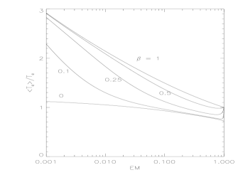
The relative importance of Coulomb heating and collisionless heating in the Sedov model just discussed can be inferred from Figure 2, where we plot the ratio of electron temperature $T_{e}$ to the mean temperature $T$ for a number of different values of parameter $\beta$. For large $\beta$, the curves are nearly straight parallel lines, with relatively unimportant Coulomb heating. The electron temperature profiles in these models are nearly the same as in the Sedov model with $\beta=1$, except for the overall temperature scaling which is proportional to $\beta$. At low $\beta$, the Coulomb heating dominates, resulting in highly curved lines. The efficiency of the Coulomb heating increases with increasing $n\Delta t/T^{3/2}$ (Itoh 1978), where $n$ is the total particle density of a fluid element, $\Delta t$ is the time elapsed since this element was shocked by the blast wave, and $T$ is the mean temperature of this fluid element. At the blast wave and in the remnant’s interior, $n\Delta t/T^{3/2}$ is small, so that the Coulomb heating is less efficient there than inside the swept shell. This is why the curves in Figure 2 attain a maximum at $EM\sim 0.5$ and drop to 0 for $EM=0$ and 1. Note that because of the scaling just mentioned, these curves are identical for all Sedov models with the same value of $\tau_{0}/T_{s}^{3/2}$.

Figure 3: Ratio of electron temperature $T_{e}$ to the mean gas temperature $T$ vs emission measure $EM$, for the Sedov model with $\eta=8.88\times 10^{51}$ ergs cm^-6, at five different times (increasing from bottom to top). Curves are labeled by the postshock temperature. Two cases with $\beta=0$ (solid curves) and $\beta=0.5$ (dotted curves) are shown.

Figure 4: Normalized ionization timescale $\tau$ vs normalized emission measure $EM$ for Sedov models.

The temperature profiles presented in Figures 1 and 2 are merely examples, with a fixed value of $\tau_{0}/T_{s}^{3/2}$, which sample a small range of the possible parameter space $(\beta,\ \tau_{0}/T_{s}^{3/2})$. The effects of varying $\tau_{0}/T_{s}^{3/2}$ are shown in Figure 3 for the same parameter $\eta$ as in Figures 1 and 2, but at different times in the remnant’s evolution (1/4, 1/2, 1, 2, and 4 of $5\times 10^{11}$ cm^-3 s). The requirement of constant $\eta$ demands that $T_{s}$ is equal to $3\times 10^{7}~{}{\rm K}/(n_{0}t/5\times 10^{11}~{}{\rm cm}^{-3}~{}{\rm s})^{6/5}$. Two cases of $\beta=0$ and 0.5 are shown. At early times, the fast collisionless heating in a model with $\beta=0.5$ dominates the Coulomb heating, leading to very different electron temperature profiles than for $\beta=0$. This is the case discussed until now. The temperature profiles become similar at later stages in the remnant’s evolution, depending rather weakly on $\beta$, because of the increased role of the Coulomb energy transfer. At $\tau_{0}=20\times 10^{11}$ cm^-3 s (curves at the top of Figure 3), noticeable differences are seen only in the remnant’s interior, where densities are low and temperatures are high, leading to a long electron-ion equlibration time scale. Note again that these temperature profiles are identical for all Sedov models with the same values of $\tau_{0}/T_{s}^{3/2}$ and $\beta$.

2.3 Ionization Calculations

The ionization state of each fluid element depends on its ionization timescale $\tau=\int_{t_{s}}^{t_{0}}n_{e}d\,t$, where $t_{s}$ is the time when this fluid element was shocked, and on how the electron temperature $T_{e}$ varied as a function of its ionization time scale, from 0 to $\tau$, during the remnant’s evolution. The normalized ionization timescale $\tau/\tau_{0}$ is plotted in Figure 4. It starts at zero at the shock ($EM=1$), then increases linearly in the swept SNR shell, but in the remnant’s interior it is again small because of low gas densities there. Note that the distribution of $\tau$ is quite broad, and is poorly represented by a $\delta$ function (the approximation involved in using a single-ionization-timescale NEI model). The most highly ionized atomic species are usually found near the maximum of $\tau$, while the least ionized material is found just behind the shock and in the remnant’s interior. We determined the electron temperature as a function of $\tau$ for each fluid element following the procedure described above.

We tracked the ionic states in each fluid element by solving the time-dependent ionization equations for each abundant element (C, N, O, Ne, Mg, Si, S, Ca, Fe, and Ni). We used an eigenfunction method to solve these equations efficiently (Masai 1984, Hughes & Helfand 1985, Kaastra & Jansen 1993, Borkowski et al. 1994). Physical processes included in these calculations are collisional ionizations by electrons, both direct and involving excitations followed by autoionizations, and radiative and dielectronic recombinations. We used collisional ionization rates from Arnaud & Raymond (1992) for Fe, and from Lennon et al. (1987) for other elements. We also updated recombination rates in the Hamilton & Sarazin (1984) X-ray code. Radiative recombination rates were taken from Péquignot, Petitjean, & Boisson (1991), and rates for dielectronic recombination towards He-like, Li-like, and Be-like ions from Hahn (1993), and Teng, Xu, & Zhang (1994a,b). Recombination rates for Fe ions were taken from Arnaud & Raymond (1992). Except for H and He, all elements are assumed to be neutral initially, a good approximation under most circumstances because of the insensitivity of X-ray spectra to the detailed ionization state of preshock plasma.

2.4 Spectral Code

We used an updated version of the X-ray code written by Hamilton & Sarazin (1984) to calculate X-ray spectra. We updated collision strengths for H-like ions using fits provided by Itikawa et al. (1985) for O⁺⁷ and by Callaway (1994) for other H-like ions. Collision strengths for He-like ions were taken from Sampson et al. (1983), Keenan et al. (1987), and Kato & Nakazaki (1989). We also updated atomic data for fluorescent Fe K$\alpha$ lines produced by inner-shell ionization. K-shell collisional ionization rates by electrons for all Fe ions were calculated according to Beigman, Shevelko, & Tawara (1996), and then combined with the fluorescence yields of Kaastra & Mewe (1993) to obtain strengths of fluorescent K$\alpha$ lines for Fe⁺⁰ – Fe⁺²¹. The fluorescent yield for Fe⁺²² was taken from theoretical calculations of transition probabilities and autoionization rates by Seely, Feldman, & Safronova (1986). Energies, transition probabilities, and excitation rates by electrons for Fe L-shell transitions for Fe⁺¹⁶ – Fe⁺²³ were kindly provided to us by Duane Liedahl (see Liedahl, Osterheld, & Goldstein 1995 and Mewe, Kaastra, & Liedahl 1995 for the description of these theoretical calculations and their implementation into the equilibrium ionization thermal MEKAL model).

2.5 Sedov Models in XSPEC

Modeling X-ray spectra of SNRs within the framework of Sedov models demands an efficient interface between observations and the calculated model spectra. Such an interface is provided by the well-known and widely-used software package XSPEC (Arnaud 1996). We wrote efficient FORTRAN programs for calculations of Sedov X-ray spectra, using methods and techniques just described, and constructed Sedov models in XSPEC v9 and v10. (The most recent version of these models was implemented by Keith Arnaud into XSPEC v11.) The model parameters are: post-shock temperature $T_{s}$, post-shock electron temperature $T_{e}$, ionization timescale $\tau_{0}$, and elemental abundances. Following standard practice used with thermal models in XSPEC, there are two versions of Sedov models, where heavy-element abundances may be varied individually or together.

Calculations of Sedov models are computationally intensive, resulting in very long computational times when X-ray data sets are fitted with these models. An even more troublesome aspect is the lack of smooth convergence when fitting with Sedov models. Keith Arnaud solved this problem by modifying a routine in the FTOOLS software package which was used to tabulate MEKAL model. With this routine we can now tabulate spatially-integrated Sedov models in a FITS file, which can then be used in conjunction with a standard XSPEC model “atable” to make fits to the data. This procedure is necessary for the robust performance of the Sedov models in XSPEC.

2.6 Calculated Spectra: Effects of Collisionless Electron Heating

The flexible computer interface provided by the XSPEC package allows us to easily generate Sedov X-ray spectra in the whole parameter space relevant for SNRs, in the energy range from 0.1 keV to 30 keV, and to simulate observations using spectral response matrices and effective areas of modern X-ray satellites. There are clearly a number of interesting issues associated the use of Sedov models, a lot of them discussed in detail by Hamilton et al. (1983), which can be efficiently examined within the XSPEC package. Here we restrict ourselves to the effects of collisionless electron heating on X-ray spectra of SNRs.

Figure 5: X-ray spectra for Sedov models with $\eta=8.88\times 10^{51}$ ergs cm^-6 and with various amounts of collisionless heating: full electron-ion equipartition (solid curve), no collisionless heating of electrons at the shock (dashed curve), and partial electron heating at the shock with the postshock electron temperature $T_{es}=0.5T_{s}$ (dotted curve). Models are displaced from each other by a factor of 10 in the vertical direction and they are labeled by the postshock temperature (in keV).

X-ray spectra for Sedov models with $\eta=8.88\times 10^{51}$ ergs cm^-3 are shown in Figure 5 at different times during the remnant evolution, and at each time for three values of $\beta$: 0.0, 0.5, and 1.0. All spectra were folded through the pre-launch instrumental response of the back-illuminated ACIS CCD detector (S3) onboard the Chandra Observatory, and include variations of the telescope’s effective area with the photon energy. The second set of spectra from the top of Figure 5 corresponds to models whose electron temperature profiles are shown in Figure 1. These spectra differ substantially from each other, and become harder with the increasing amount of collisionless heating. Particularly large differences are seen at high energies, reflecting large differences in temperature profiles seen in Figure 1. It should be obvious that, in general, it is necessary to consider not only the extremes of very efficient and completely inefficient electron heating, but also models with partial electron heating at the shock.

Differences between X-ray spectra of Sedov models with different amounts of collisionless heating become smaller as the remnant ages, because of the increased role of the Coulomb heating in older remnants without full electron-ion equilibration at the shock front (see Figure 3). This is clearly seen in Figure 5, where there is hardly any difference between the coolest models with and without collisionless heating. Most of the X-ray emitting plasma in these models is actually not very far from coronal equilibrium ionization.

3 INTERPRETATION OF X-RAY SPECTRA

X-ray and UV spectra of stellar coronae showed the presence of multi-temperature hot plasmas, which led researchers to consider temperature distribution functions in their efforts to understand the observed coronal spectra. This approach proved quite useful in analysis of X-ray spectra of stellar coronae. It would be advantageous to have a similar framework available for SNRs, so we generalized the idea of the temperature distribution function used for plasmas in ionization equlibrium to NEI Sedov models.

3.1 Temperature and Ionization-Timescale Distribution Functions

The spatially-integrated X-ray spectra for Sedov models can be succesfully interpreted in terms of the following three distributions: the electron temperature, ionization timescale, and ionization timescale-averaged electron temperature distribution functions. We have already shown the ionization timescale distribution in Figure 4, and examples of the electron temperature distribution in Figure 1. These two distributions do not contain enough information to determine ionic states, because of the adiabatic expansion of the gas following its passage through the blast wave. This expansion results in a decreasing mean temperature for each fluid element. This is demonstrated in Figure 6, where we plot temperature variations for several fluid elements in the Sedov model. Particularly large variations are seen for fluid elements which were shocked early in the remnant’s evolution. Another reason for electron temperature variations is energy transfer from ions to electrons in models with unequal ion and electron temperature. In principle a detailed account of the electron temperature variations is needed for each fluid element, just as we did for Sedov models, but a simpler approach in terms of an average temperature provides a better insight while maintaining good accuracy. A suitable average electron temperature is the ionization timescale-averaged temperature $\langle T_{e}\rangle$, defined as $\int_{t_{s}}^{t_{0}}T_{e}(t)n_{e}(t)dt/\tau$. In Figure 7, we plot the ratio $\langle T_{e}\rangle/T_{e}$ for Sedov models with $T_{s}=3\times 10^{7}$ K, $\tau_{0}=5\times 10^{11}$ cm^-3 s, and various amounts of collisionless electron heating. For equal ion and electron temperatures this ratio is significantly greater than unity in the remnant’s interior because of the adiabatic expansion. In the opposite limit of no collisionless heating, $\langle T_{e}\rangle$ is slightly less than $T_{e}$ in the postshock region, because the efficient transfer of energy from ions to electrons more than compensates for adiabatic expansion. However, even in this case the temperature ratio becomes larger than unity in the remnant’s interior, demonstrating the effectiveness of the adiabatic expansion. After passing through the shock front, electrons in a fluid element are heated by Coulomb collisions with ions, but because of the adiabatic expansion the efficiency of Coulomb heating decreases, and the electron temperature attains a maximum and then starts to decline with time. Even modest amounts of collisionless heating affect the ionization timescale averaged distribution function in the remnant’s interior and at the shock front (Fig. 7), where the ionization timescale is low and the Coulomb heating is least effective (Fig. 2). As the collisionless heating becomes more important, the ratio $\langle T_{e}\rangle/T_{e}$ increases until it reaches its upper limit in fully equilibrated models.

Figure 6: Temperature of fluid elements in the Sedov model, normalized to their final values, vs normalized ionization timescale $\tau/\tau_{0}$. The temperature history is shown for 4 different fluid elements (solid curves), labeled by their normalized emission measure $EM$. A linear approximation discussed in the text is also shown (dotted curves).

Figure 7: Ratio of ionization timescale-averaged electron temperature $\langle T_{e}\rangle$ to final electron $T_{e}$ vs emission measure $EM$ for Sedov models shown in Figures 1 and 2, and with various amounts of collisionless heating. Curves are labeled by $\beta$.

Figure 8: Ratio of ionization timescale-averaged electron temperature $\langle T_{e}\rangle$ to final electron $T_{e}$ vs emission measure $EM$ for Sedov models shown in Figure 5, with $\eta=8.88\times 10^{51}$ ergs. Two cases with $\beta=0$ (solid curves) and $\beta=0.5$ (dotted curves) are shown. Curves are labeled by the shock temperature. Dashed curve corresponds to model with full electron-ion equilibration.

The temperature profiles presented in Figure 7 are again merely examples, with a fixed value of $\tau_{0}/T_{s}^{3/2}$, which sample a small range of the possible parameter space $(\beta,\ \tau_{0}/T_{s}^{3/2})$. The effects of varying $\tau_{0}/T_{s}^{3/2}$ are shown in Figure 8, for Sedov models with electron temperature distribution functions shown in Figure 3. The ionization timescale averaged distributions differ from each other, reflecting the relative importance of adiabatic cooling and Coulomb heating at various locations within the remnant. However, they are all bounded from below by models with low efficiency of Coulomb heating and no collisionless heating, and from above by models with equal ion and electron temperatures.

The two temperatures, the electron temperature $T_{e}$ and the average electron temperature $\langle T_{e}\rangle$, may be used to obtain an approximate functional relationship of electron temperature with ionization timescale for each fluid element. A linear relationship is simple and sufficient, starting with temperature $2\langle T_{e}\rangle-T_{e}$ at the shock (ionization timescale equal to 0), and ending with $T_{e}$ at the current local ionization timescale $\tau$. We show this linear approximation in Figure 6 for a model with equal ion and electron temperatures. The agreement with the exact Sedov solution is excellent for the bulk of the X-ray emitting material, although it becomes somewhat less accurate in the remnant’s interior where temperature variations are more pronounced. This approximate description of electron temperature variations allows us to calculate ionization fractions and then X-ray spectra, and compare them with the exact X-ray calculations for Sedov models described in § 2.6. We find excellent agreement between the two sets of calculations for models with equal ion and electron temperatures, with typical differences at most of order of few percent (for cosmic abundance Sedov models at the ASCA or Chandra CCD spectral resolution). The agreement is slightly worse for models without any collisionless heating, but the differences are rarely at the $\sim 10$% level and they are limited to a few line complexes at lower energies. Because such differences are smaller than current uncertainties in atomic data, we did not find it necessary to develop a more accurate approximation to describe the evolution of electron temperature in a fluid element. The current linear approximation is clearly sufficient for calculations of X-ray emission from the Sedov blastwave. While it offers negligible computational advantages over exact calculatons for Sedov models, we find it useful for interpretation of X-ray spectra. This approximate description may also be very convenient in more complex situations, which might require multi-dimensional hydrodynamical simulations.

X-ray spectra of SNRs are apparently described very well by the electron temperature, ionization timescale, and ionization timescale averaged electron temperature distribution functions. High-quality X-ray data may allow us to determine these distribution functions without reliance on detailed hydrodynamical calculations. This is analogous to determinations of differential emission measure in stellar coronae, without reliance on coronal models. The experience gained in analysis of stellar coronae suggests that such an empirical approach should be useful in analysis of X-ray spectra of SNRs. But instead of one temperature distribution function needed in a stellar corona, three distribution functions are required to describe NEI X-ray spectra of SNRs. A purely empirical determination of these distribution functions might then be a difficult task, so we expect that its combination with hydrodynamical modeling will prove most useful in the future.

3.2 Constant Temperature, Single Ionization Timescale Models

Figure 9: Fits to X-ray spectra of Sedov models of Figure 3, for clarity displaced from each other by factor of 10 and shown by solid curves (top – $T_{es}=T_{s}$, middle – $T_{es}=0.5T_{s}$, bottom – $T_{es}=0$). A constant temperature, single ionization timescale model (dotted curves) provides a poor fit when compared with plane-parallel shock (dashed curves).

The most common NEI model in use today is the constant temperature, single ionization timescale model. In terms of the distribution functions just discussed, electron temperature and average electron temperature are assumed constant, and the ionization distribution shown in Figure 4 is approximated by a delta function. As already noted by researchers (e. g., Masai 1994), the latter approximation is particularly troublesome. If it is used to describe a plane-parallel shock or a Sedov model, prominent lines produced by strongly underionized plasma immediately behind the shock will be missing from the model spectrum. This is demonstrated in Figure 9, where we again show the calculated X-ray spectra for Sedov model with solar abundances, and with the same parameters as in Figures 1 and 7 ($T_{s}=3\times 10^{7}~{}{\rm K}=2.59~{}{\rm keV},\tau=5\times 10^{11}$ cm^-3 s). We fitted a simple NEI model just described to these spectra, using the XSPEC software package, and the best fits are shown in Figure 9. The very poor match between the calculated spectra and the best fit model spectra demonstrates that the model under consideration is not adequate to represent X-ray spectra of SNRs. The current practice of using the constant temperature, single ionization timescale NEI model to represent X-ray spectra of SNRs is not valid in general. This simple NEI model may be used judiciously under special circumstances, e. g., for an isolated dense cloud of gas overrun by a shock long time ago or for SN ejecta in old remnants which were thermalized early in the remnant’s evolution. However, these are exceptions to the rule because X-ray emission in SNRs is generally produced behind shocks, much as in Sedov models.

3.3 Plane-Parallel Shock Models

The failure of a constant temperature, single ionization timescale model is caused by an improper approximation of the ionization timescale distribution (Fig. 4) by the delta function. A broad distribution such as seen in Figure 4 is needed in order to provide a good approximation to Sedov models. A simple and obvious choice is a plane-parallel shock characterized by a constant postshock electron temperature $T_{e}$ and by its ionization age $\tau_{s}=n_{e}t_{s}$, where $n_{e}$ is the postshock electron density and $t_{s}$ is the shock age. This model differs from a single ionization timescale NEI model in its linear distribution of ionization timescale vs emission measure (at the shock the ionization timescale is 0, and it attains the maximum $\tau_{s}$ for the material shocked earliest). Such a simple shock provides a much better approximation to the Sedov models shown in Figure 9, where we also plot the best fit shock model. The difference between Sedov models and the shock model is noticeable only at low energies, particularly for models with no collisionless electron heating. For equal ion and electron temperatures, final values of the free parameters of the fit give a very good approximation to the mean electron temperature ($T_{e}=3.26$ keV vs the emission-weighted electron temperature of $1.27T_{s}=3.29$ keV in the Sedov model) and the mean ionization timescale ($\tau_{s}/2=9.88\times 10^{10}$ cm^-3 s vs $\langle\tau\rangle=0.202\tau_{0}=1.01\times 10^{11}$ cm^-3 s, where $\langle\tau\rangle$ is the emission-measure averaged ionization timescale in Sedov models). Reasonable agreement is also obtained for the other two nonequipartition models with $T_{es}=0.5T_{s}=1.30$ keV and $T_{es}=0$: shock temperatures 2.15 keV and 1.58 keV vs the emission-weighted electron temperatures of $0.74T_{s}=1.91$ keV and $0.53T_{s}=1.37$ keV in Sedov models, and $\tau_{s}/2=7.84\times 10^{10}$ cm^-3 s, $6.50\times 10^{10}$ cm^-3 s vs $1.01\times 10^{11}$ cm^-3 s in Sedov models. This example demonstrates that plane-parallel shocks might serve as useful approximations to Sedov models with high electron temperatures in the Chandra spectral range. From the computational point of view, plane-parallel shocks with constant electron temperature require little computational overhead when compared with the single ionization timescale model (when ionic states are calculated with the eigenfunction technique). But unlike the latter model, plane-parallel shocks are useful for fitting X-ray spectra in a broad range of model parameters.

Plane-parallel shocks with constant electron temperatures just discussed constitute a subclass of more general plane shocks with partial electron heating at a shock. Electrons are also heated by collisions with ions downstream of the shock, just as in Sedov models. These shocks may be parametrized by the shock temperature $T_{s}$, the postshock electron temperature $T_{es}$, and the shock ionization age $\tau_{s}$. If $T_{s}=T_{es}$, we arrive at constant-temperature shock models discussed above. The case with no collisionless heating at the shock corresponds to $T_{es}=0$, where Coulomb collisions gradually lead to increase in the electron temperature $T_{e}$ downstream of the shock, which becomes equal to $T_{s}$ in the limit of the infinite shock ionization age $\tau_{s}$, far from the shock front. For partial electron heating at the shock, $0<\beta=T_{es}/T_{s}<1$, just like for Sedov models.

Multitemperature, plane-parallel shock models with unequal electron and ion temperatures at the shock should generally provide better fits to Sedov models. We find that this is indeed true, in particular, we can obtain perfect fits to Sedov models in Figure 9. For $T_{es}=0.5T_{s}=1.30$ keV, the best plane-parallel shock fit gives $T_{s}=5.57$ keV, $T_{es}=0.82$ keV, $\tau_{s}/2=1.08\times 10^{11}$ cm^-3 s, and emission weighted electron temperature $T_{e}=0.37T_{s}=2.04$ keV. For $T_{es}=0$, we get $T_{s}=3.36$ keV, $T_{es}=0$, $\tau_{s}/2=9.66\times 10^{10}$ cm^-3 s, and emission weighted electrom temperature $T_{e}=0.44T_{s}=1.46$ keV. It may be seen that while $T_{s}$ and $T_{es}$ cannot be reliably determined by fitting shocks to Sedov models of Figure 9, the derived emission weighted $T_{e}$ and the SNR ionization age $\tau_{0}$ compare well with parameters of the Sedov model.

Figure 10: X-ray spectra for Sedov models with $\eta=10^{50}$ ergs cm^-6 and with equal ion and electron temperatures, for clarity displaced from each other by a factor of 10 in the vertical direction. Curves are labeled by the postshock temperature (in keV). The best fit shock models (dottted curves) compare well with Sedov models (solid curves) at high temperatures, but they differ significantly at low temperatures.

The excellent agreement between plane-parallel shocks and Sedov models at high electron temperatures, demonstrated in Figure 9, does not hold at low shock velocities. In Figure 10, we show X-ray spectra for an SNR with $\eta=n_{0}^{2}E=10^{50}$ ergs cm^-3 and equal ion and electron temperatures, at various times during its evolution. The best fit spectra produced by a plane-parallel, constant electron temperature shock are also shown. The fits are perfect early in the remnant’s evolution, at high shock temperatures, but they deteriorate as the blast wave decelerates. Particularly large differences are seen at high energies, where the shock model spectrum is too soft. This is not suprising because high energy emission in Sedov models is produced at significantly higher temperatures than at the shock, as can be seen from the electron temperature distribution function in Figure 1. Constant temperature plane parallel shocks provide a poor approximation to this multitemperature distribution function, and should not be generally used to fit X-ray spectra of low temperature Sedov models in the 0.1 – 10 keV spectral range.

3.4 Multitemperature NEI Models

An inadequate representation of the distribution functions is the reason why single ionization timescale NEI models in general, and plane-parallel shocks at low shock speeds, fail to reproduce X-ray spectra of Sedov models. In the latter, it is the presence of multitemperature plasma in Sedov models (see Figures 1 and 7) which is responsible for this failure. It is possible to construct two-temperature, three-temperature, and generally multi-zone “simple” NEI models which provide a good approximation to X-ray spectra of Sedov models, provided that these models are consistent with the three distribution functions discussed previously. We constructed such models succesfully, and found that at most $\sim 10$ temperature zones are needed for Sedov models at low temperatures, while just a couple might be sufficient at intermediate and high temperatures. While such multitemperature NEI models might possibly be useful for computational reasons, they have been designed as a method of successive approximation (more temperature zones give a better model), and not by a physical simplicity. For this reason we advocate the use of full Sedov models, and not multi-zone models, in modeling of spatially-integrated X-ray spectra of SNRs, because Sedov models represent a simple physical situation of a spherical blast wave propagating into a uniform ambient medium. However, multi-zone models most likely will be very useful in spatially-resolved X-ray spectral modeling of SNRs.

4 DETERMINATION OF MODEL PARAMETERS FROM X-RAY SPECTRA

There are three parameters of Sedov models which may be determined from spatially integrated X-ray spectra: postshock temperature $T_{s}$, postshock electron temperature $T_{es}$, and the ionization age $\tau_{0}$ (plus chemical abundances which we do not discuss here). It is generally difficult to determine all three parameters, particularly when observations are available only in a limited X-ray spectral range or when deviations from the Sedov dynamics are present. We will first consider two limiting cases of young and hot, and much older and cooler SNRs.

When young and hot remnants are observed in the 0.1 – 10 keV spectral range, such as provided by the Chandra CCDs, most of the emission comes from the bulk of the X-ray emitting material, with emission measures between 0.1 – 1.0, located behind the blast wave. Because of the low ionization timescales characteristic of young remnants, the electron temperature distribution function is generally flat and has a similar shape for models with various amounts of electron heating in this range of emission measures (see Figures 1 and 2). The ionization timescale averaged electron temperature distributions are also similar (Figure 7), while the ionization timescale distributions are of course identical and reasonably well approximated by a straight line (Figure 4). We have already shown that under these conditions plane parallel shocks with constant electron temperature provide an excellent approximation to Sedov models in the 0.1 – 10 keV energy range. This demonstrates that the observed X-ray spectrum depends mostly on the mean electron temperature in the postshock region and on the ionization timescale $\tau_{0}$. It is difficult to determine $T_{s}$ and $T_{es}$ separately without additional information. Observations at higher energies, which would probe interior regions where the temperature distribution functions differ between the models (see Figure 1), are not likely to succeed because of expected severe deviations from the Sedov dynamics in the interior regions of young remnants.

It is possible to determine independently the shock speeds in young remnants through high spectral resolution observations. The postshock radial velocity of the bulk of the X-ray emitting material is equal to $0.75v_{s}$, which results in a velocity difference of $1.5v_{s}$ between the front and back section of the shell at the remnant’s center. With a sufficient spectral resolution, Doppler-shifted spectral lines originating in these two shell sections could be separated, providing us with the missing information about the shock speed. This straightforward kinematic measurement is currently hard to accomplish because of the lack of X-ray instrumentation with a sufficiently high spectral resolution for spatially-extended sources such as SNRs. Such measurements would provide us with the shock temperature, which in combination with the analysis described above would allow for a complete determination of Sedov model parameters. Note that the high spectral resolution would also provide additional electron temperature and ionization timescale diagnostics based on individual line ratios.

Additional information about postshock velocities and postshock electron temperatures can also be independently found from optical and UV observations of nonradiative, Balmer-dominated shocks. The width of the broad H$\alpha$ component seen in these shocks is a direct measure of the postshock proton temperature. In combination with X-ray observations, this is enough information to determine the shock speed in young remnants. In addition, UV and optical lines in such shocks are produced by electron impact excitation, (although in the fastest shocks proton excitation might also be important), and carefully chosen line ratios can be good diagnostics of postshock electron temperatures. This is a poweful method for determining both temperatures from optical observations alone, although it is limited to shocks with a nonnegligible population of neutral H atoms entering the shock front. But for such fast nonradiative shocks one can find a complete set of shock parameters from optical, UV, and X-ray observations.

In contrast to hot and young SNRs just discussed, low shock temperatures and large ionization timescales in old remnants lead to efficient Coulomb heating and ion-electron equilibration. Departures from equilibration are important only in the immediate vicinity of the shock and in the remnant’s interior (e.g., see top of Figure 3). Spatially-integrated X-ray spectra for models with the same postshock temperature $T_{s}$ but different $T_{es}$ differ significantly only at high energies, as shown in Figure 5 for a model with $kT_{s}=0.49$ keV and $\eta=8.88\times 10^{51}$ ergs cm^-6. The postshock temperature $T_{s}$ and the ionization timescale $\tau_{0}$ (or parameter $\eta$) can be obviously found from the shape of the X-ray spectrum at low energies. But determination of the postshock electron temperature $T_{es}$ must rely on the high-energy X-ray spectrum. The high-energy spectrum is produced by hot gas in the remnant’s interior which was shocked early in the evolution of the remnant when departures from the Sedov dynamics could be significant. In this situation, it might be difficult to distinguish between effects of collisionless electron heating and effects of departures from the Sedov dynamics, particularly for remnants with low shock temperatures $T_{s}$ and large ionization timescales $\tau_{0}$. For such remnants, determination of both $T_{s}$ and $T_{es}$ is best accomplished through spatially-resolved X-ray, UV, and optical spectroscopy in the narrow region immediately behind the shock front (e. g., see Ghavamian 1999; Ghavamian et al. 2000).

Figure 11: X-ray spectra for Sedov models with $T_{s}=0.6$ keV and with various amounts of collisionless heating: full electron-ion equipartition (solid curve), no collisionless heating of electrons at the shock (dashed curve), and partial electron heating at the shock with $T_{es}=0.5T_{s}=0.3$ keV (dotted curve). Models are displaced from each other by a factor of 10 in the vertical direction and they are labeled by the ionization timescale $\tau_{0}$ (in cm^-3 s).

The postshock electron temperature $T_{es}$ and the postshock temperature $T_{s}$ can be simultaneously determined from spatially-integrated spectra for remnants with intermediate shock temperatures and low ionization timescales $\tau_{0}$. We demonstrate this in Figure 11, where we show calculated X-ray spectra for Sedov models with the postshock temperature $T_{s}=0.6$ keV, with three values of $T_{es}$ (0 keV, 0.3 keV, and 0.6 keV), and for $\tau_{0}$ ranging from $3\times 10^{10}$ cm^-3 s to $3\times 10^{12}$ cm^-3 s. (Again, the calculated spectra were folded through the spectral response of the back-illuminated ACIS CCD detector.) Note that the plane-parallel shock model provides a poor approximation to these spectra because of the relatively low (0.6 keV) postshock temperature. X-ray spectra for models with low values of $\tau_{0}$ show strong dependence on $T_{es}$, particularly at high energies, because of the lack of ion-electron equilibration. For such remnants, a simultaneous determination of $T_{s}$ and $T_{es}$ from spatially-integrated X-ray spectra should be possible. As the ionization timescale $\tau_{0}$ increases, Coulomb heating becomes effective, and the effects of collisionless electron heating decrease in importance. For large ionization timescales $\tau_{0}$, spectra in Figure 11 depend little on $T_{es}$, and determination of $T_{es}$ becomes difficult.

5 SUMMARY

We discussed spatially-integrated X-ray spectra of SNRs based on Sedov dynamics. Their spectral shape depends on elemental abundances and on three parameters: postshock temperature $T_{s}$, postshock electron temperature $T_{es}$, and ionization timescale $\tau_{0}$ (or parameter $\eta$). These three parameters can in principle be determined by comparing models with observations for any remnant, but frequently only one of the postshock temperatures can be found. Only the postshock electron temperature $T_{es}$ can be usually determined for young, hot remnants, and only the shock temperature $T_{s}$ can be found for old, much colder SNRs. In order to find both $T_{s}$ and $T_{es}$ for such SNRs, additional information about the shock is necessary, such as available from kinematic studies or from UV and optical observations. It should be possible to determine both $T_{s}$ and $T_{es}$ from the spatially-integrated spectrum alone for SNRs with intermediate temperatures and ionization timescales.

We succesfully explained differences between X-ray spectra for Sedov models with different parameters in terms of three distribution functions: the electron temperature distribution, the ionization timescale distribution, and the ionization-timescale averaged electron distribution. We then considered a number of simple models, such as a single ionization timescale model and plane-parallel shock models, and compared their distribution functions and X-ray spectra with Sedov models. A frequently used single ionization timescale model was found to be an inappropriate approximation to Sedov models. In most situations, plane-parallel shocks provide a much better approximation to Sedov models, and both plane shocks and Sedov models should be routinely used in analysis of SNR X-ray spectra.

The NEI models described in this work, while constituting a basic set of simplest thermal models, are not sufficient for interpretation of SNR spectra. A single plane parallel or a spherical shock is a crude approximation to the complex morphology of SNRs seen in X-ray images. For complex morphologies, observed X-ray spectra are most likely a superposition of shocks with various velocities, resulting in distribution functions which are poorly described by a single shock. In general, we do not expect that the NEI models presented here can provide perfect or even statistically acceptable fits to SNR spectra, because of deviations from an idealized plane shock or a Sedov model. This is indeed the case for DA 530 (Landecker et al. 1999), 3C397 (Safi-Harb et al. 2000) and RCW 86 (Borkowski et al. 2000), SNRs whose X-ray spectra were modeled with plane shocks and Sedov models. More effort is clearly necessary in order to take full advantage of X-ray observations of SNRs. Improved modeling must involve a superposition of shocks with various speeds or determination of distribution functions directly from observed X-ray spectra, a challenging task because of the modest spectral resolution of CCD detectors onboard Chandra or XMM-Newton.

We based our X-ray emission calculations on Sedov-Taylor dynamics, in which shocks are not modified by cosmic rays. But if collisionless shocks were strongly modified in SNRs (Jones & Ellison 1991), then their dynamics would be poorly described by the Sedov-Taylor self-similar solution, and the resulting X-ray emission could be very different than in standard Sedov models. Dorfi & Böhringer (1993) and more recently Decourchelle, Ellison, & Ballet (2000) showed that the cosmic-ray modification of shock structure can indeed have a dramatic effect on X-ray spectra of SNRs. This is not suprising because a significant amount of energy is deposited into relativistic particles in cosmic-ray dominated shocks, which results in lower temperatures of thermal gas. In several models calculated by Berezhko et al. (1994, 1996), the energy fraction contained in cosmic rays may be as high as 80% of the total SNR kinetic energy. We found that in such extreme cosmic-ray dominated SNRs the thermal gas temperature is too low for production of substantial amounts of thermal X-ray emission, except early in the remnant’s evolution when its dynamics and X-ray emission are strongly affected by SN ejecta. Futhermore, we generally found flat temperature profiles in such models, because of a higher fraction of energy deposited into cosmic rays at higher shock velocities. Such approximately isothermal SNRs differ greatly from Sedov models, which generally contain the hottest gas in their interiors. In terms of our distribution functions, the electron temperature distribution is flat in these isothermal SNRs, the ionization timescale is larger because of the increased postshock compression ratio, but the shape of the ionization timescale distribution is similar to that seen in Figure 4. Because of adiabatic expansion, the ionization-timescale averaged temperature is qualitatively the same as depicted in Figures 6 and 7.

These trends should be also present in other cosmic-ray modified SNR models with lower particle acceleration efficiencies. A lower efficiency is actually possible because the idealized, spherically-symmetric models calculated by Berezhko et al. assume a quasiparallel shock everywhere along its periphery, in which particle acceleration is most efficient. But realistic SNR blast waves must consist of a mixture of quasiparallel and quasiperpendicular shocks, and in the absence of strong turbulence, quasi-perpendicular shocks may not accelerate particles as efficiently. It is then likely that “only” $\sim 50$% of the SNR kinetic energy is transferred to cosmic rays (Evgeny Berezhko, private communication), in which case thermal gas will produce appreciable amounts of X-ray emission during the late adiabatic evolutionary stage of interest here. But such SNRs must have significantly different distribution functions than standard Sedov models, so that they must produce significantly different X-ray spectra. A considerable caution is then required when modeling and interpreting X-ray observations of SNRs. The distribution functions presented by us are valid only for Sedov models, without any shock modification by cosmic rays. It would be worthwhile to carry out an extensive investigation of the distribution functions expected in various cosmic-ray dominated SNR models, but this task clearly demands a separate effort. Note that, unlike for Sedov models, X-ray spectra produced by our plane-parallel shocks may be used even for cosmic-ray modified shocks. The only difference is in interpretation of the shock temperature $T_{s}$, whose relationship with the shock velocity $v_{s}$ is now provided not by the standard Rankine-Hugoniot shock jump conditions, but by jump conditions appropriate for a collisionless shock with a particular cosmic-ray acceleration efficiency.

Another issue connected with the cosmic ray acceleration in SNRs is the question of the electron velocity distribution. In our X-ray emission modeling we assumed that thermal electrons can be well described by a Maxwellian velocity distribution. This is most likely a good assumption for the bulk of electrons, usually referred to as thermal electrons, but the presence of radio synchrotron emission in SNRs demonstrates that there is a high energy tail to this distribution. The most energetic ($\sim$ 10 – 100 TeV) electrons produce nonthermal synchrotron X-ray emission, as has been recently inferred for SN 1006 (Koyama et al., 1995), Cas A (Allen et al., 1997), G347.5-0.2 (Slane et al., 1999), and RCW 86 (Borkowski et al. 2000), and modeled in detail by Reynolds (1998). In addition, less energetic electrons in the high energy tail, with energies of several tens of keV, can also produce lines and continua, through the same atomic processes as thermal electrons. (The continuum produced by such electrons is usually referred as nonthermal bremsstrahlung.) If these nonthermal processes are important in an SNR, then interpretation of its X-ray spectrum must rely on a combination of thermal and nonthermal models. A good example is SNR RCW 86 where a complex mixture of nonthermal synchrotron and multitemperature thermal emission is present (Borkowski et al. 2000). It is not clear at this time how important nonthermal bremsstrahlung is in SNRs, because of the predominance of nonthermal synchrotron X-ray emission. But if nonthermal bremsstrahlung were important, energetic electrons producing it would also excite line emission, possibly leading to changes in line strength ratios and intensities. The possible presence of such electrons in SNRs is clearly an important issue for interpretation of SNR X-ray spectra. One might hope that with the high quality X-ray observations of SNRs becoming available, we will be able to determine the distribution functions discussed in this work, and unambiguously separate thermal and nonthermal emission in SNRs.

References

- Allen et al. (1997) Allen, G. E., et al. 1997, ApJ, 487, L97
- Arnaud (1996) Arnaud, K. A. 1996, in Astronomical Data Analysis and Systems V, eds. G.Jacoby & J.Barnes, ASP Conf. Series, v.101, 17
- Arnaud & Raymond (1992) Arnaud, M., & Raymond, J. 1992, ApJ, 398, 394
- Beigman et al. (1996) Beigman, I. L., Shevelko, V. P., & Tawara, H. 1996, Physica Scripta, 53, 534
- Berezhko et al. (1994) Berezhko, E. G., Yelshin, V. K., & Ksenofontov, L. T. 1994, APh, 2, 215
- Berezhko et al. (1996) Berezhko, E. G., Yelshin, V. K., & Ksenofontov, L. T. 1996, ARep, 40, 155
- Borkowski et al. (1994) Borkowski, K. J., Sarazin, C. L., & Blondin, J. M. 1994, ApJ, 429, 710
- Borkowski et al. (2000) Borkowski, K. J., Rho, J., Reynolds, S. P., & Dyer, K. K. 2000, ApJ, submitted
- Bykov & Uvarov (1999) Bykov, A. M., & Uvarov, Yu. A. 1999, J. of Experimental and Theoretical Physics, 88, 465
- Callaway (1994) Callaway, J. 1994, At. Data Nucl. Data Tables, 57, 9
- Cox & Anderson (1982) Cox, D. P., & Anderson, P. R. 1982, ApJ, 253, 268
- Decourchelle et al. (2000) Decourchelle, A., Ellison, D. C., & Ballet, J. 2000, ApJ (Letters), in press
- Dorfi & Böhringer (1993) Dorfi, E. A., & Böhringer, H. 1993, A&A, 273, 251
- Ghavamian (1999) Ghavamian, P. 1999, PH.D Thesis, Rice University
- Ghavamian et al. (2000) Ghavamian, P., Raymond, J., Smith, R. C., & Hartigan, P. 2000, ApJ, in press
- Gronenschild & Mewe (1982) Gronenschild, E. H. B. M., Mewe, R., 1982, ApJ, 48, 305
- Hahn (1993) Hahn, Y. 1993, J. Quant. Spectrosc. Radiat. Transfer, 49, 81
- Hamilton et al. (1983) Hamilton, A. J. S., Sarazin, C. L., Chevalier, R. A. 1983, ApJS, 51,115
- Hamilton & Sarazin (1984) Hamilton, A. J. S., & Sarazin, C. L. 1984, ApJ, 284, 601
- Hughes et al. (1998) Hughes, J. P., Hayashi, I., & Koyama, K. 1998, ApJ, 505, 732
- Hughes & Helfand (1985) Hughes, J. P., & Helfand, D. J. 1985, ApJ, 291, 544
- Itikawa et al. (1985) Itikawa, Y., Hara, S., Kato, T., Nakazaki, S., Pindzola, M. S., & Crandall, D. H. 1985, At. Data Nucl. Data Tables, 33, 149
- (23) Itoh, H. 1978, PASJ, 30, 489
- (24) Itoh, H. 1979, PASJ, 31, 541
- Jones & Ellison (1991) Jones, F. C., & Ellison, D. C. 1991, Space Sci. Rev., 58, 259
- Kaastra & Jansen (1993) Kaastra, J. S., & Jansen, F. A. 1993, A&AS, 97, 873
- Kaastra & Mewe (1993) Kaastra, J. S., & Mewe, R. 1993, A&AS, 97, 443
- Kato & Nakazaki (1989) Kato, T., & Nakazaki, S. 1989, At. Data Nucl. Data Tables, 42, 313
- Keenan et al. (1987) Keenan, F. P., McCann, S. M., & Kingston, A. E. 1987, Physica Scripta, 35, 432
- Koyama et al. (1995) Koyama, K., Petre, R., Gotthelf, E. V., Hwang, U., Matsura, M., Ozaki, M., Holt, & S. S. 1995, Nature 378, 255
- Laming et al. (1996) Laming, J. M., Raymond, J. C., McLaughlin, B. M., & Blair, W. P. 1996, ApJ, 472, 267
- Landecker et al. (1999) Landecker, T. L., Routledge, D., Reynolds, S. P., Smegal, R. J., Borkowski, K. J., & Seward, F. D. 1999, ApJ, 527, 866
- Lennon et al. (1988) Lennon, M. A., Bell, K. L., Gilbody, H. B., Hughes, J. G., Kingston, A. E., Murray, M. J., & Smith, F. J. 1988, J. Phys. Chem. Ref. Data, 17, 1285
- Liedahl et al. (1995) Liedahl, D. A., Osterheld, A. L., & Goldstein, W. H. 1995, ApJ, 438, L115
- Lyerly et al. (1997) Lyerly, W. J., Reynolds, S. P., Borkowski, K. J., & Blondin, J. M. 1997, BAAS, 29, 839
- Masai (1984) Masai, K. 1984, Ap&SS, 98, 367
- Masai (1994) Masai, K. 1994, ApJ, 437, 770
- Mewe et al. (1995) Mewe, R., Kaastra, J. S., & Liedahl, D. A. 1995, Legacy, 6, 16
- Péquignot et al. (1991) Péquignot, D., Petitjean, P., & Boisson, C. 1991, A&A, 251, 680
- Reynolds (1998) Reynolds, S. P. 1998, ApJ, 493, 375
- Safi-Harf et al. (2000) Safi-Harb, S., Petre, R., Arnaud, K. A., Keohane, J. W., Borkowski, K. J., Dyer, K. K., Reynolds, S. P., & Hughes, J. P. 2000, ApJ, in press
- Sampson et al. (1983) Sampson, D. H., Goett, S. J., & Clark, R. E. H. 1983, At. Data Nucl. Data Tables, 28, 467
- Sedov (1946) Sedov, L. I. 1946, Prikl. Mat. Mekh., 10(2), 241
- Seely, Feldman, & Safronova (1986) Seely, J. F., Feldman, U., & Safronova, U. I. 1986, ApJ, 304, 838
- Slane et al. (1999) Slane, P. , Gaensler, B. M., Dame, T. M., Hughes, J. P., Plucinsky, P. P. & Green, A. 1999, ApJ, 525, 357
- Taylor (1950) Taylor, G. I. 1950, Proc. Roy. Soc. A, 201, 159
- (47) Teng, H., Xu, Z., & Zhang, W. 1994a, Physica Scripta, 49, 463
- (48) Teng, H., Xu, Z., & Zhang, W. 1994b, Physica Scripta, 49, 696