PMN J1838–3427: A new gravitationally lensed quasar

Abstract

We report the discovery of a new double-image quasar that was found during a search for gravitational lenses in the southern sky. Radio source PMN J1838–3427 is composed of two flat-spectrum components with separation $1\farcs 00$, flux density ratio 14:1 and matching spectral indices, in VLA and VLBA images. Ground-based $BRI$ images show the optical counterpart (total $I=18.6$) is also double with the same separation and position angle as the radio components. An HST/WFPC2 image reveals the lens galaxy. The optical flux ratio (27:1) is higher than the radio value probably due to differential extinction of the components by the lens galaxy. An optical spectrum of the bright component contains quasar emission lines at $z=2.78$ and several absorption features, including prominent Ly-$\alpha$ absorption. The lens galaxy redshift could not be measured but is estimated to be $z=0.36\pm 0.08$. The image configuration is consistent with the simplest plausible models for the lens potential. The flat radio spectrum and observed variability of PMN J1838–3427 suggest the time delay between flux variations of the components is measurable, and could thus provide an independent measurement of $H_{0}$.

1 Introduction

The new double-image quasar presented in this paper is the first to result from a program that three of us (J.N.W., J.N.H., and P.L.S.) began to find new radio-loud gravitational lenses in the southern sky. Our main goal is to find suitable lenses for time-delay measurements. The time delays between the flux variations of the multiple images of a gravitationally lensed quasar can be used as a “one-step” measurement of the Hubble constant $H_{0}$ (Refsdal, 1964) or, more precisely, a combination of angular-diameter distances between the Earth, lens galaxy, and quasar (for recent reviews see Myers (1999); Williams & Schechter (1997)). In addition, the measured lensing rate in a well-defined sample of extragalactic sources places interesting limits on the cosmological constant (Fukugita et al. (1992); Kochanek (1996); Falco et al. (1998)).

Our search methodology will be described in a future paper; we confine ourselves here to a summary. We selected southern sources because the southern hemisphere is relatively unexplored for lenses and therefore more likely to contain bright and useful specimens. The southern limit is $\delta=-40\arcdeg$ to permit the use of the NRAO Very Large Array (VLA) and Very Long Baseline Array (VLBA), instruments that facilitate the search.

We selected only sources with flat spectral indices ($\alpha\geq-0.5$, where $S_{\nu}\propto\nu^{\alpha}$) as measured between the 4.85 GHz Parkes-MIT-NRAO catalog (Griffith & Wright, 1993) and the 1.4 GHz NRAO VLA Sky Survey (Condon et al., 1998, NVSS). Flat-spectrum sources tend to be core-dominated, and therefore variable (a prerequisite for measuring time delays), easily recognized when lensed, and easily mapped by an automatic procedure. In this respect our program is similar to the Cosmic Lens All-Sky Survey (CLASS; Myers et al. (1995)), a program that (after including the sample of the Jodrell-VLA Astrometric Survey, JVAS) has identified at least 15 new lenses among 15000 northern-hemisphere radio sources.

We observed each object for 30 seconds at 8.46 GHz with the VLA in its A configuration. Objects exhibiting multiple compact components (about 5% of the sample) were selected as lens candidates and scheduled for appropriate follow-up observations, including multifrequency VLA imaging, VLBA imaging, and optical imaging. The goal of the follow-up observations is to determine whether the components have similar spectral properties and surface brightnesses (as lensed images should) and to search for a lens galaxy.

For the particular case of PMN J1838–3427, the chronology of observations was as follows. The initial VLA image from 1998 May 19 contained two compact components separated by $1\farcs 00$. The most likely explanation for this morphology was a core-jet or core-hotspot structure. However, in ground-based images obtained during 1999 April 10-15, the optical counterpart was revealed to be a double with the same separation and position angle as the radio double, thereby suggesting PMN J1838–3427 was either a binary quasar or a gravitational lens.

On 1999 July 19, multifrequency observations with the VLA revealed that the spectral indices of the components were the same. This evidence favored the gravitational lens hypothesis, since lensing is achromatic. We used the VLBA on 1999 October 11 to search for matching milliarcsecond substructure within the radio components, which is characteristic (although not required) of lensed images. Both components were detected, but no matching substructure was seen.

On the strength of the evidence thus far, PMN J1838–3427 was included in the CfA-Arizona Space Telescope Lens Survey (CASTLES), an effort by seven of us (E.E.F., C.D.I., C.S.K., J.L., J.A.M., B.A.M., and H.-W.R.) to use the Hubble Space Telescope (HST) to observe all the known galaxy-scale gravitational lenses. The HST/WFPC2 image, obtained on 2000 March 1, revealed a diffuse light source between the quasar components which is naturally interpreted as a lens galaxy. This left no doubt that PMN J1838–3427 is a gravitationally lensed quasar.

We obtained optical spectra of the quasar and lens galaxy with the ESO 3.6m telescope at La Silla on 2000 March 4. This allowed us to measure the source redshift $z=2.78$ but our lens galaxy spectrum was inconclusive. Finally, in order to assess the radio variability of PMN J1838–3427 we measured its total flux at two frequencies with the Australia Telescope Compact Array (ATCA) on 2000 April 5.

Subsequent sections of this paper present these observations in logical rather than chronological order. Sections 2 through 4 present the radio properties of the system, as revealed by measurements with the VLA, VLBA, and ATCA. Sections 5 and 6 present space- and ground-based optical images, and § 7 presents optical spectra of the quasar and lens galaxy. We consider simple models of the lens potential in § 8. Finally, in the last section we review the evidence that PMN J1838–3427 is a gravitationally lensed quasar and discuss the prospects for measuring and interpreting the time delay between its lensed images.

2 VLA images

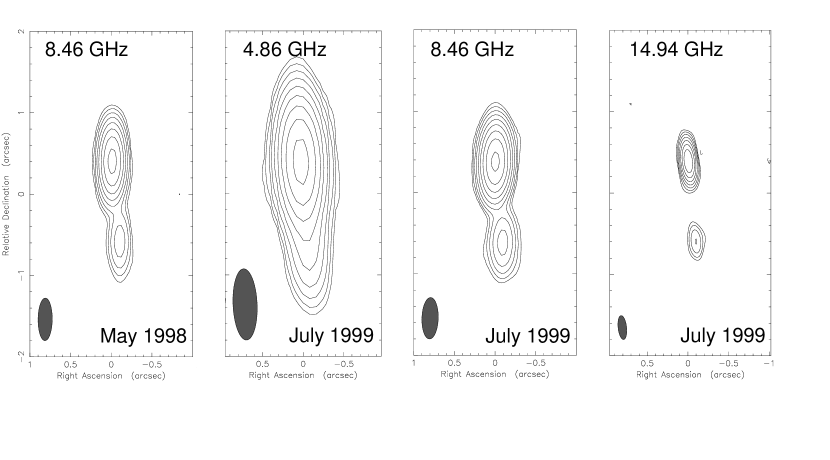
Figure 1: VLA images (2″$\times$ 4″) of PMN J1838–3427. Contours begin at $3\sigma$ and increase by powers of 2, where $\sigma$ is the RMS level in the residual map. From left to right $\sigma=0.35$, 0.20, 0.24, and 0.49 mJy/beam. The restoring beams (inset in the lower left of each map) are elongated N/S due to low-elevation observing. Beam diameters are listed in column 3 of Table 1.

The date, frequency, resolution, and sensitivity of the VLA observations are listed in the first four rows of Table 1. In all cases the VLA was in its A configuration and the total observing bandwidth was 100 MHz. Radio source 3C286 was used to set the absolute flux scale, following the procedures suggested in the VLA Calibrator Manual and adopting flux densities 7.49, 5.52, and 3.42 Jy at 4.86, 8.46, and 14.94 GHz respectively. Calibration was performed with standard procedures in AIPS. Deconvolution and imaging were performed with Difmap (Shepherd et al., 1994). This included phase-only self-calibration with a 30-second solution interval. The final images, created with uniform weighting and an elliptical Gaussian restoring beam, are shown in Figure 1.

In each image there are two components. Throughout this paper we refer to the northern component of PMN J1838–3427 as A, and the southern component as B. To measure the separation and flux density ratio of A and B, we fit a two-component model to the self-calibrated visibilities using the “modelfit” utility of Difmap. After subtracting the best-fit model from the data, the residual images were all consistent with thermal noise.

The best-fit parameters are listed in Table 1. The flux density ratios are in rough agreement but are not equal within the quoted uncertainties. For a gravitational lens the ratios are expected to be approximately equal, but one reason to expect small discrepancies is variability of the background object (see § 9 for further discussion). Two-point spectral indices were computed for each component based on the 1999 July 19 observations. The results are listed in Table 2. Both components are verified to have flat radio spectra.

The coordinates of component A, based on the 1999 July 19 images, are R.A. (J2000)$~{}=18^{{\mathrm{h}}}38^{{\mathrm{m}}}28^{{\mathrm{s}}}.50$, Dec. (J2000) $=-34\arcdeg 27\arcmin 41\farcs 6$, within $0\farcs 2$.

3 VLBA image

We observed PMN J1838–3427 for 4 hours with the VLBA on 1999 October 11. The St. Croix and Brewster antennas were unavailable. The observing bandwidth was 48 MHz, divided into 8 IFs, with an average frequency of 4.975 GHz. The visibility averaging time was 1 second. This level of spectral and time sampling was sufficient to prevent significant bandwidth- and time-average smearing over the required field of view.

Calibration was performed with standard procedures in AIPS. Fringe fitting for sources with widely spaced components is problematic without a prior model of the source, because the source structure causes rapid time variation of the solutions. For this reason we used a two-step procedure. First, the data were fringe-fitted using a point source model and a 30-second solution interval. This allowed a preliminary image to be made, in which components A and B were both detected. Then, the calibration was redone by fringe-fitting with reference to a two-component model based on the preliminary image and a 3-minute solution interval. The final images were created with Difmap, after repeated iterations of model fitting and phase-only self-calibration.

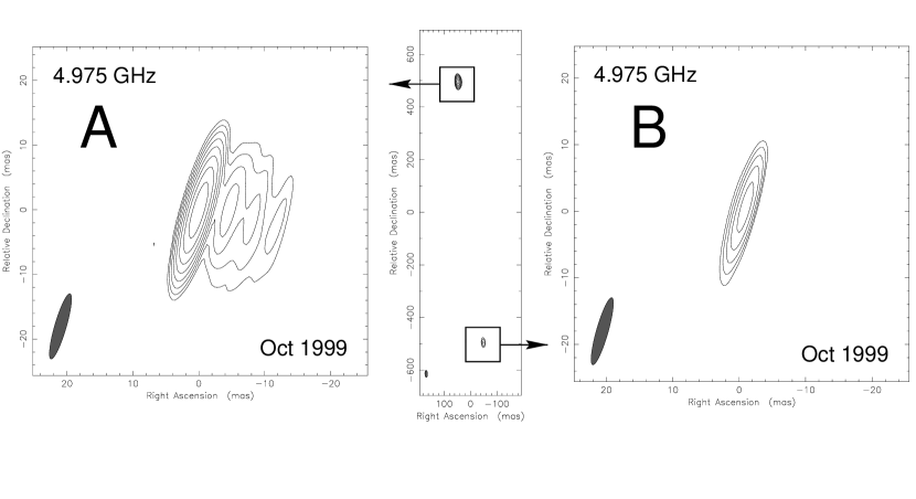
Figure 2: VLBA image of PMN J1838–3427. A wide-field image, displaying both northern and southern components, is displayed in the center panel. Close-ups of the northern and southern components are shown in the left and right panels, respectively. Contour levels begin at $3\sigma$ and increase by powers of 2, where $\sigma$ is the RMS level in the residual map, which is 0.20 mJy/beam near A and 0.18 mJy/beam near B. The synthesized beam, depicted in the lower left of each map, has FWHM diameters 10.5 $\times$ 1.8 mas.

The final uniformly-weighted images are shown in Figure 2. Both a wide-field map and close-ups of each component are displayed. Component B is unresolved. Component A is partially resolved; in addition to an unresolved component there is extended emission to the west, comprising about 10% of the total flux density.

A model for the surface brightness distribution was constructed with Difmap, by fitting a circular Gaussian to each compact component (which we continue to identify as A and B), and then using the Clean algorithm to account for the diffuse emission west of A with a large number of point sources. During the subsequent iterations of model-fitting and self-calibration, the Clean components were kept fixed and the circular Gaussian parameters were varied. The best-fit positions and flux densities of A and B are reported in the last entry of Table 1. The separation between the Gaussian components is 996.1 mas and the position angle is $5\fdg 59$ east of north. The total flux density of the diffuse emission is 16.7 mJy.

The flux density of B is the same in the VLBA and VLA images, but the flux density of A is 27% smaller in the VLBA image. As a result the VLBA flux density ratio (10.6) is smaller than the VLA ratios (which average 14.6). Even when the total flux density of the diffuse emission west of A is added to that of A, the VLBA ratio is only 11.8. One possible explanation is that the VLA image of A includes relatively diffuse flux that is missing from the VLBA image. The shortest VLBA baseline (236 km, or 4 M$\lambda$) is longer than the longest VLA baseline (35 km, or 0.6 M$\lambda$), so there is a range of spatial frequencies that are unresolved by the VLA and invisible to the VLBA. Another possibility to explain part or all of the discrepancy is that the source varied between observing epochs. Due to the time delay between components, source variability would cause fluctuations in the instantaneous flux density ratio.

Since PMN J1838–3427 is a gravitational lens, there should be radio emission east of B corresponding to the emission west of A. However, given the peak brightness of the emission west of A (2.5 mJy/beam) and the magnification ratio described above, one would expect the brightness of such emission to be at most 0.24 mJy/beam, which is not much higher than the RMS level of 0.18 mJy/beam. Confirmation of matching milliarcsecond substructure will require deeper imaging.

4 ATCA measurements

To test for variability we examined PMN J1838–3427 with the Australia Compact Telescope Array (ATCA) on 2000 April 5, observing simultaneously at 4.80 and 8.64 GHz while the array was in the 6D configuration. The observation was divided into three scans of one minute each, with 2 hours between scans to improve the $uv$-coverage. Calibration was performed with the software package MIRIAD, and imaging with Difmap. The absolute flux density scale was set by observations of PKS B1934–638, which is believed to match the 3C286-based flux scale within 3%.

The antenna spacings were not large enough to resolve the components, so we used the VLA models to fix the separation of the two components and varied their flux densities to achieve the best fit to the ATCA data. Since the individual flux densities are covariant we report only their sum in Table 3. The uncertainty was estimated as the quadrature sum of the range in total flux obtained by analyzing each one-minute scan separately, and a 3% uncertainty due to absolute flux calibration. Table 3 also lists other flux density measurements reported in this paper and in various published radio catalogs.

The total ATCA flux density at 4.80 GHz was the same as the most recent 4.86 GHz VLA measurement. However, the total flux density at 8.64 GHz was 44% higher than the most recent 8.46 GHz VLA measurement, indicating strong variability. (The expected difference due to spectral index alone is 0.6%, and the combined measurement uncertainty is 5%.) Variability at 8.46 GHz is corroborated by the 12% variation in total flux density observed between the two VLA measurements.

5 HST image

On 2000 March 1, three dithered exposures (700 sec, 700 sec, 600 sec) of PMN J1838–3427 were acquired during one HST orbit, using the Wide Field and Planetary Camera 2 (WFPC2) and the F814W filter. The data were reduced with the standard CASTLES pipeline: the exposures were registered, weighted by exposure time, and combined using a 3-sigma “ccdclip” rejection algorithm. (See Lehár et al. (2000) for other examples of two-image lenses observed in the CASTLES program.)

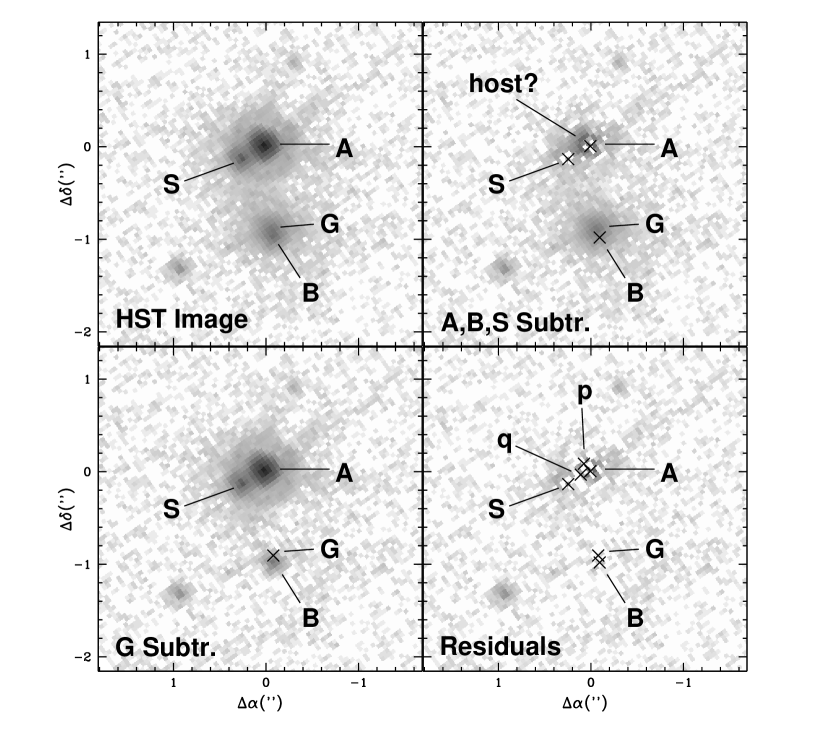
Figure 3: Upper left. HST/WFPC2 image of PMN J1838–3427 through filter F814W ($\approx I$). Here and in all other panels, the gray levels are logarithmically scaled. Upper right. Same, but with components A, B and S subtracted in order to highlight the lens galaxy G. The residuals near A are tentatively identified as due (at least in part) to the quasar host galaxy. Lower left. Only component G has been subtracted, in order to highlight the dim quasar component B. Lower right. All model components have been subtracted. There are still residuals near A possibly due to the host galaxy.

The upper left panel of figure 3 is a 3″$\times$ 3″ subraster of the final image. Components A and B are present with the same separation and position angle as the corresponding radio components. Crucially, the southern component is not compact. There is diffuse emission extending northward from B towards A, which is labeled G. The natural interpretation is that G is a lens galaxy: it lies along the line joining A and B, and its position near B is consistent with the large flux density ratio between A and B (see § 8 for simple models).

In addition, there is a third compact object $0\farcs 28$ southeast of A, labeled S. Object S is almost certainly not a third image of the background quasar, because it is silent in all our radio images. In particular, the 4.86 GHz image of 1999 July 19 requires S to be at least 200 times dimmer than A, whereas in the optical image it is about 8 times dimmer. Missing optical images can be plausibly explained by dust extinction (e.g. B1152+199; Myers et al. (1999)) but missing radio images defy simple explanation.

The low galactic latitude ($b=-12\arcdeg$) of the field suggests that S is a foreground star. To estimate the a posteriori probability of a star intruding on the lens, we estimated the local mean density of stars by counting all the stars in the PC field (32″$\times$ 32″) that are at least as bright as S. Based on this mean density, the probability that at least one star would appear within $0\farcs 5$ of component A, component B, or the line joining them, is 5%. This is somewhat low but within reason.

To measure the relative positions and magnitudes of A, B, G, and S, we created parameterized models of the image using a twice-oversampled PSF created by TinyTim v4.4 (Krist & Hook, 1997). The models were fit to the data using the procedures of Lehár et al. (2000). The first model contained three point sources (representing A, B, and S) and a circular de Vaucouleurs profile (G). The residual image contained a diffuse pattern of residuals centered on component A with an integrated flux equal to 12% of the combined flux of A and S, suggesting that A is not adequately modeled by a point source. Possibly, the host galaxy of the background quasar and/or additional foreground objects are contributing light.

We tried accounting for this extra light with additional model components, such as a circular de Vaucouleurs profile, an elliptical de Vaucouleurs profile, and extra point sources. There is no compelling reason to recommend one of these models over the others, but we judged that the residuals appeared most random for a model with two extra point sources. We refer to these two extra point sources as p and q. The best-fit parameters of the model are listed in Table 4. Parameter uncertainties were estimated in the same manner as Lehár et al. (2000): three terms were added in quadrature, representing the statistical error in the fit, the range in parameters obtained with different choices of the model PSF, and the range obtained with two different modeling programs.

The upper right panel of Figure 3 shows the image after components A, B and S of the best-fit model have been subtracted. This allows the lens galaxy G and the excess residuals near A to be seen clearly. In the lower left panel, only G has been subtracted, highlighting component B. It is worth noting that the A/B flux ratio in this image (27:1) is much higher than any of the radio flux density ratios. This is probably due to the proximity of B and G. Optical extinction due to the lens galaxy should be greater for component B than for A.

In the lower right panel the entire model (including p and q) has been subtracted. There are still residuals near A, extending in both directions nearly perpendicular to the A/B separation. The elongation of the residuals is suggestive of tangentially-stretched emission from a host galaxy. Deeper HST or adaptive-optics imaging in the infrared will be useful to clarify the nature of the putative host galaxy.

To connect the WFPC2 photometry to the Johnson-Kron-Cousins system we approximated F814W $\approx I$ and adopted a zero-point magnitude of 21.69, as did Lehár et al. (2000). This zero-point is based on the calibration of Holtzmann et al. (1995), but with a gain of 7 and a correction of 0.1 mag for finite aperture. The resulting magnitude of component A is $I=19.21$, and the total magnitude of all components is $I=18.79$, with a scatter of 0.05 between different models and an additional uncertainty of at least 0.05 due to the choice of zero-point magnitude.

6 Ground based optical images

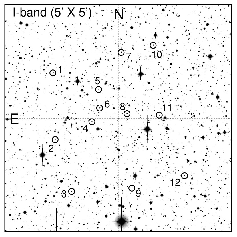
Figure 4: Wide-field (5′$\times$ 5′) $I$-band image centered on PMN J1838–3427. The 12 reference stars discussed in § 6 are circled and numbered. Magnitudes and positions of these stars, relative to star #8, are provided in Table 6.

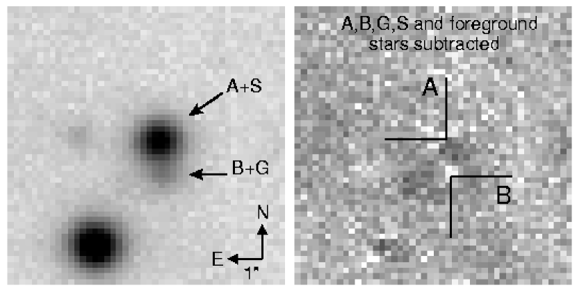
Figure 5: Left. Ground-based $I$-band image (8″$\times$ 8″) of PMN J1838–3427. Components A and S are unresolved, as are components B and G. There are foreground stars to the southeast and east. Gray levels are logarithmically scaled from $-5\sigma$ (white) to the central intensity of PMN J1838–3427 (black). Right. Residual image after a six-component model describing PMN J1838–3427 and the foreground stars (see § 6) has been subtracted. For clarity, only the positions of A and B are marked. Gray levels are linearly scaled from $-5\sigma$ to $+5\sigma$.

During 1999 April 10-14 we obtained $BRI$ images of PMN J1838–3427 with the du Pont 2.5m telescope at Las Campanas Observatory (LCO). We used the SITe#3 $2048\times 4096$ CCD camera, with gain 2.5 e^-/D.N. and read noise 6.6 e^-. Table 5 is a journal of these observations. The images were bias-subtracted and flat-fielded with standard IRAF procedures. The rotation and pixel scale ($0\farcs 1631$) of each image were derived using at least 30 stars from the USNO-A2.0 catalog (Monet et al., 1999). Figure 4 shows the $5\arcmin\times 5\arcmin$ $I$-band field. The left panel of Figure 5 is an $8\arcsec\times 8\arcsec$ subraster centered on PMN J1838–3427.

Photometry was performed with the DAOPHOT package in IRAF. First, we constructed an empirical PSF using the signal-weighted average of the images of 12 well-exposed, widely-spaced stars in the field. These reference stars are circled and labeled in Figure 4. Due to the crowded condition of the field, the PSF diameter was limited to $5\arcsec$. Next, we used this PSF template to fit simultaneously for the positions and magnitudes of all 12 reference stars, all the components representing PMN J1838–3427, and all the neighbors of the reference stars and PMN J1838–3427 within $5\arcsec$.

For the $I$ and $R$ images the model of PMN J1838–3427 consisted of four point sources representing A, B, G, and S. Their relative positions were fixed at the values measured in the HST image. For the $B$ images, which had poorer seeing and a smaller signal, the covariance between A and S and between B and G prevented convergence. For these we used a model consisting of two components with the same relative separation as A and B in the HST image.

The right panel of Figure 5 shows the $I$-band image at high contrast after subtraction of the best-fit model. The neighboring stars to the southeast and east were also subtracted. A pattern of positive residuals between A and B at the $4\sigma$ level may be unmodeled light from G. In all other images the residuals were consistent with noise.

The instrumental magnitudes of the reference stars and components of PMN J1838–3427, relative to reference star #8, are listed in Table 6. The quoted uncertainty in each magnitude difference is the statistical error in the fit. For a few stars in the $R$ and $B$ images the uncertainty was increased to encompass the difference between fits to the two different exposures. We emphasize that the magnitudes of A and S are covariant, as are those of B and G. Components A and S were typically separated by just one-third of the seeing disc and B and G by only one-tenth. For this reason, the combined magnitudes of A+S and of B+G are also listed in Table 6.

We connected the instrumental magnitudes to the Johnson-Kron-Cousins photometric system by observing at least one of the standard fields described by Landolt (1992) each night. Six stars in the field SA110-499 were used to calibrate the $B$ and $R$ magnitude scales, using the $B-R$ index to compute color terms. Four stars in PG0918+029 and three stars in PG1323–086 were used to calibrate the $I$ magnitude scale, using the $R-I$ index to compute color terms. In all cases the aperture diameter was $14\arcsec$. We adopted “typical” Las Campanas extinction coefficients of $k_{I}=0.08$, $k_{R}=0.11$, and $k_{B}=0.28$. The calibrated magnitudes of reference star #8 are printed beneath Table 6. The quoted uncertainty is the quadrature sum of the uncertainty in the instrumental magnitude and the RMS scatter in the calibration solution. With this calibration, the total apparent magnitudes of all model components (A, B, S, and G) during 1999 April 10-14 were $I=18.56$, $R=19.16$, and $B=20.48$, within 0.04 mag.

The total $I$ magnitude disagrees with the value derived from the HST/WFPC2 image ($I=18.79\pm 0.07$). More significantly, the LCO image exhibits a much larger contrast between northern (A+S) and southern (B+G) components. In the LCO image the flux ratio (A+S)/(B+G) is $8.3\pm 0.3$, whereas the WFPC2 value is $4.6\pm 0.4$. These discrepancies are possibly the result of variability of the source quasar. However, the significance of these discrepancies is unclear, since the results were derived from different instruments and photometric models. Repeated ground-based measurements will be important in assessing variability, using Table 6 as a baseline.

7 Optical spectroscopy

Optical spectra of the quasar and lens galaxy were obtained with the 3.6m telescope of the European Southern Observatory (ESO) at La Silla, Chile. We used the ESO Faint Object Spectrograph and Camera (EFOSC) with CCD #40 ($2048\times 2048$, gain 1.3 e^-/D.N., readout noise 7.5 e^-) and grism #6 (3860-8070Å, 30 gr/mm) giving a plate scale of 2Å per pixel. We obtained two separate spectra, one in which the slit was centered on quasar component A and one centered on the lens galaxy G. In both cases the slit was $0\farcs 7$ wide and oriented east-west in order to isolate the components as much as possible.

The quasar spectrum is shown in the top panel of Figure 6. It was obtained on 2000 March 4 in a 30-minute exposure in $1\farcs 8$ seeing, through an airmass of 1.5 and has a resolution of 10Å. No attempt was made to correct for differential atmospheric refraction. Three broad emission lines are obvious, corresponding to Ly$\alpha$ (1216Å), Si IV+O IV (1400Å), and C IV (1549Å) at a redshift of $2.78\pm 0.01$. This redshift was determined with reference to the Si IV+O IV and C IV lines only, since the broad absorption trough blueward of Ly-$\alpha$ makes centroid estimation difficult. Once this redshift was established, a probable emission line of C III] (1909Å) was identified.

At least two significant non-terrestrial absorption lines are also present in the spectrum (4890Å and 5000Å), but we are unable to assign them confidently to systems at particular redshifts. We did not identify any $z=0$ stellar absorption lines in this spectrum, which would have confirmed the hypothesis of § 5 that component S is a foreground Galactic star. This is not surprising, because the A/S flux ratio is 8.1 in the HST image while the signal-to-noise ratio of each resolution element is only 7.5.

The lens galaxy spectrum, shown in the bottom panel of Figure 6, was obtained on 2000 March 6 with a 60-minute exposure through an average airmass of 1.5 in 1$\farcs$3 seeing. The resolution has been degraded to 30Å by combining wavelength bins, in order to boost the signal-to-noise. The slit also admitted the southern quasar component B, but based on the HST photometric model (Table 4) the light from G was expected to dominate B.

There is only one definite feature, an emission line at 6560Å with a S/N of about 3. This feature does not appear in the quasar spectrum, which has been scaled to the level expected from the B component and plotted as a dotted line in Figure 6. Although the wavelength of this feature is suspiciously close to $z=0$ H$\alpha$, suggesting it might result from imperfect background subtraction, there were several brighter sky lines that were subtracted successfully. It is therefore tempting to identify this feature with emission from the lens galaxy.

With one line of unknown origin, redshift determination is impossible. However, it is possible to estimate the lens galaxy redshift from photometry alone, by requiring the photometric properties to be consistent with the passively-evolving fundamental plane (FP) of early-type galaxies. Kochanek et al. (2000) described the FP method and applied it to 17 lenses with known spectroscopic redshifts, finding a scatter of 0.11 between the FP and spectroscopic redshifts. Applied to PMN J1838–3427, the lens galaxy redshift estimate is $z_{FP}=0.36\pm 0.08$. Given this redshift estimate, one plausible identification for the emission at 6560Å is [O III] (5007Å) at $z=0.31$. The emission line appears to be resolved, which could be a result of blending with [O III] (4959Å) and/or H$\beta$ (4861Å). In this case one would expect to see these lines in a deeper spectrum, along with [O II] (3727Å) at 4882Å. A redder spectrum would reveal H$\alpha$ (6563Å) at 8598Å.

Obviously there are many other possibilities, if the lens redshift is not correctly predicted by the FP method. Nevertheless, for the purpose of lens modeling (§ 8) we adopt $z_{l}=0.36$ as a working hypothesis.

8 Models of the lens potential

The present observations of PMN J1838–3427 provide only five useful constraints on the lens potential: the positions of B and G relative to A in the HST/WFPC2 image (Table 4) and the A/B radio flux density ratios (Table 1). The optical magnitude differences are not useful because they are affected by dust extinction, reddening and possibly microlensing in the lens galaxy. Any additional lensed images must be dimmer than A by a factor of at least 200, based on the radio images. We therefore confine ourselves to simple two-image models.

Our first purpose is to confirm that lensing is a natural explanation for the observed image configuration. For this purpose we consider the simplest plausible model for the dark-matter halo of a galaxy, an isothermal sphere. This model produces two images with a magnification ratio equal to the ratio of their distances from the lens center. The lens galaxy center in the HST/WFPC2 image is displaced 8 mas east of the line joining A and B (see Table 4); this is within the positional uncertainty, so an isothermal sphere is a viable model.

The image separations in Table 4 imply a magnification ratio of $11.8\pm 1.7$. This compares well with the radio flux density ratios in Table 1, although it is only in actual agreement with the VLBA ratio. There is a good reason why one might expect the VLBA flux density ratio to correspond more closely to the magnification ratio: it may exclude relatively diffuse flux that is lumped into component A in the VLA images (see § 3). Another possible explanation for the small but significant discrepancies is source variability. The proper comparison to the magnification ratio is not the instantaneous flux density ratio, but rather the ratio of light curves that have been shifted by the appropriate time delay.

Our second purpose is to model the system in the same manner as other two-image lenses observed in the CASTLES program (Lehár et al., 2000), for the sake of uniformity and to provide the starting point for more detailed models. Although the rough agreement with the isothermal sphere model is encouraging, it would be naive to conclude that it is an adequate model for the lens potential. Numerous studies have shown that, while an isothermal sphere provides a good first approximation, extra terms representing internal or external shear must be added at the 10-20% level to match all the observational constraints (Keeton, Kochanek & Seljak, 1997). We therefore consider a singular isothermal ellipsoid (SIE), in which the surface mass density is (in units of the critical surface density for lensing),

$$\kappa(x,y)=\frac{b}{2}\left[\frac{2q^{2}}{1+q^{2}}\left(x^{2}+y^{2}/q^{2}\right)\right]^{-1/2},$$ (1)

where $q$ is the axis ratio and $b$ sets the mass scale.

There are five parameters ($b$ and $q$ as above, and three implied parameters for the position angle of the axes and the source coordinates). Since there are also five constraints, the parameters are determined uniquely. We chose the mean of the radio flux density ratios listed in Table 1 as the constraint on the magnification ratio, with the caveats discussed above. We determined parameter uncertainties by surveying the range of parameters for which $\Delta\chi^{2}<1$. The results are listed in Table 7.

We used this model to predict the quantity $h\Delta t$, where $\Delta t$ is the time delay and $H_{0}=100h$ km/s/Mpc. The prediction depends on the lens galaxy redshift, the cosmological parameters $\Omega_{m}$ and $\Omega_{\Lambda}$, and the clumpiness of matter on cosmological scales. For the lens galaxy redshift we adopt the FP estimate $z_{l}=0.36$ (see § 7). Under the further assumptions $\Omega_{m}=0.3$ and $\Omega_{\Lambda}=0.7$, and using the filled-beam approximation, $h\Delta t=14.9\pm 0.2$ days. If instead $\Omega_{m}=1$ and $\Omega_{\Lambda}=0$ then $h\Delta t=14.0\pm 0.2$ days. The quoted uncertainties are based on the SIE model only, and are therefore underestimates; many authors have shown that a wider class of lens models needs to be explored to obtain realistic error estimates (e.g. Kochanek (1991); Bernstein & Fischer (1999); Williams & Saha (1999)).

9 Summary and future prospects

We now summarize the argument that PMN J1838–3427 is a gravitational lens. It consists of two flat-spectrum radio components, each of which is compact on milliarcsecond scales and has a stellar optical counterpart. This implies both components are quasars, and indeed the bright component is a spectroscopically verified $z=2.78$ quasar. Radio-loud quasars are scarce enough that when two of them are observed within $1\arcsec$, they are probably either a physical binary or a pair of lensed images. That the spectral indices of each component are the same suggests lensing is the explanation. A high-resolution optical image shows diffuse emission (the lens galaxy) along the line between the components. The image configuration is consistent with the simplest plausible mass distribution for the lens galaxy.

Will this new lens be useful in the enterprise of using time delays to constrain cosmological parameters and/or aspects of galaxy structure? The answer depends on whether the time delay of PMN J1838–3427 can be measured and whether more constraints on the potential of the lens galaxy are likely to be discovered.

As for the first issue, measuring the time delay, prospects are good. There are several indications that PMN J1838–3427 is variable at radio wavelengths. Its spectral index is flat and the components are compact on milliarcsecond scales, both of which are indicators of variability. In addition, the three measurements of total flux density at 8.5 GHz listed in Table 3 (two from the VLA and one from ATCA) are all significantly different. At optical wavelengths we do not have as much information to judge variability. The discrepancy between the ground-based (LCO) $I$-band photometry and the WFPC2 photometry (see § 6) is one suggestion of variability, but further monitoring is required. The local reference system established in § 6 and Table 6 will be of use in future measurements.

The second issue, constraining the lens potential, is the greater challenge. At least the lens appears to be a single galaxy, and the lens position and magnification ratio are consistent with the simplest plausible models, giving PMN J1838–3427 an advantage over more obviously complicated lenses with measured time delays, such as Q0957+561 and CLASS B1608+656. The challenge will be to obtain enough constraints to explore a wider class of models. Deeper or higher-resolution VLBI observations may reveal corresponding substructure in the lensed images. Infrared images from space or with adaptive optics will improve estimates for the lens galaxy’s position and shape. They would also clarify the nature of the host galaxy that was tentatively identified in § 5, which could provide very important model constraints (Kochanek, Keeton & McLeod, 2000). Obtaining the lens galaxy redshift is also a priority. If these observational challenges can be met, PMN J1838–3427 will contribute to the growing field of using lensing phenomena to study galaxy structure and cosmology.

Figure 6: Top. Optical spectrum of quasar component A with resolution 10Å. Dashed lines indicate emission lines at $z=2.78$. Telluric lines ($\oplus$) are also marked. Bottom. Optical spectrum of the lens galaxy with resolution 30Å. The dotted line is the quasar spectrum from the top panel, after scaling by the B/A flux ratio and adjusting for exposure time. Due to variable seeing and non-photometric conditions the scale factor is uncertain by at least 15%.

Table 1: Photometric models based on VLA and VLBA data

Date	Frequency	Beam FWHM	Flux density		RMS noise	$\Delta$R.A.	$\Delta$Decl.	Flux density
	(GHz)	(mas $\times$ mas, P.A.)	A (mJy)	B (mJy)	(mJy/beam)	(mas)	(mas)	ratio
19 May 1998	8.46	$520\times 180$ (0°)	192.0	13.7	0.35	$-94\pm 3$	$-985\pm 7$	$13.97\pm 0.35$
19 Jul 1999	8.46	$590\times 210$ ($-1$°)	169.7	11.5	0.24	$-94\pm 3$	$-998\pm 6$	$14.73\pm 0.31$
19 Jul 1999	4.86	$960\times 340$ (2°)	200.4	13.2	0.20	$-88\pm 3$	$-1013\pm 8$	$15.22\pm 0.23$
19 Jul 1999	14.94	$300\times 110$ (7°)	168.8	11.7	0.49	$-97\pm 3$	$-987\pm 7$	$14.45\pm 0.61$
11 Oct 1999	4.975	$10.5\times 1.8$ ($-16$°)	145.4	13.7	0.19	$-96.99\pm 0.04$	$-991.32\pm 0.14$	$10.61\pm 0.14$

Note. — The first four rows are based on VLA data (§ 2). The last row is based on VLBA data (§ 3). The RMS level in each image was taken as an estimate of the uncertainty in the relative flux density scale. The absolute flux density scale is uncertain by an additional 3% for the first 3 rows and 5% for the last 2 rows, based on VLA documentation. The uncertainty in each coordinate was estimated as the beam FWHM divided by twice the S/N (peak/RMS) of the component.

Table 2: Two-point spectral indices based on VLA data

Frequency 1	Frequency 2	Component A	Component B	Uncertainty due to
(GHz)	(GHz)			absolute flux scale
4.86	8.46	$-0.299\pm 0.003$	$-0.24\pm 0.05$	0.08
8.46	14.94	$-0.009\pm 0.006$	$+0.02\pm 0.08$	0.10
4.86	14.94	$-0.152\pm 0.003$	$-0.11\pm 0.04$	0.05

Note. — Spectral indices $\alpha$ are defined such that $S_{\nu}\propto\nu^{\alpha}$. Uncertainties quoted in columns 3 and 4 derive only from the RMS level in each image. Column 5 reports the additional uncertainty due to the absolute flux scales, which affects A and B identically.

Table 3: Compilation of radio flux density measurements

		Frequency	Flux density
Date	Observatory	(GHz)	A (mJy)	B (mJy)	A+B (mJy)
1974-83	UTRAO	0.365	$\cdots$	$\cdots$	$451\pm 36$
May 1996	VLA (DnC config.)	1.40	$\cdots$	$\cdots$	$280.2\pm 8.4$
1979	Parkes	2.70	$\cdots$	$\cdots$	$240$
Nov 1990	Parkes	4.85	$\cdots$	$\cdots$	$258\pm 21$
19 Jul 1999	VLA (A config.)	4.86	200.4	13.2	$213.6\pm 6.4$
11 Oct 1999	VLBA	4.975	145.4	13.7	$175.9\pm 8.8\tablenotemark{f}$
5 Apr 2000	ATCA (6D config.)	4.80	$\cdots$	$\cdots$	$218.7\pm 6.8$
19 May 1998	VLA (A config.)	8.46	192.0	13.7	$205.7\pm 6.2$
19 Jul 1999	VLA (A config.)	8.46	169.7	11.5	$181.2\pm 5.4$
5 Apr 2000	ATCA (6D config.)	8.64	$\cdots$	$\cdots$	$264.2\pm 8.6$
19 Jul 1999	VLA (A config.)	14.94	168.8	11.7	$180.5\pm 9.0$

Note. — For observations that could not resolve A and B, only the total flux density is reported.

Table 4: Photometric model based on HST/WFPC2 image

Component	$\Delta$R.A.	$\Delta$Decl.	Relative	$R_{{\mathrm{e}}{\mathrm{f}}{\mathrm{f}}}$
	(mas)	(mas)	flux	(arcsec)
A	0	0	$100\pm 6$	$\cdots$
B	$-101\pm 6$	$-987\pm 5$	$3.77\pm 0.55$	$\cdots$
G	$-85\pm 6$	$-911\pm 6$	$20.9\pm 1.3$	0.20
S	$239\pm 2$	$-140\pm 5$	$12.3\pm 1.6$	$\cdots$
p	$70\pm 11$	$81\pm 17$	$5.7\pm 2.5$	$\cdots$
q	$104\pm 8$	$-37\pm 21$	$4.7\pm 0.8$	$\cdots$

Table 5: Journal of ground-based optical observations

Date	Filter	Duration	Seeing	Airmass
		(sec)	(arcsec)
10 April 1999	$R$	600	0.81	1.02
11 April 1999	$R$	1000	0.88	1.01
11 April 1999	$B$	1000	0.92	1.01
12 April 1999	$I$	1500	0.63	1.01
14 April 1999	$B$	1800	0.88	1.01

Table 6: Photometry and astrometry of PMN J1838–3427 and 12 reference stars

Object	$\Delta$R.A.	$\Delta$Decl.	$\Delta I$	$\Delta R$	$\Delta B$
	(sec)	(arcsec)	(mag)	(mag)	(mag)
A	$0.925$	$-5.96$	$1.075(8)$	$1.002(31)$	$\cdots$
S	$\cdots$	$\cdots$	$3.238(51)$	$4.252(129)$	$\cdots$
G	$\cdots$	$\cdots$	$3.616(220)$	$4.009(264)$	$\cdots$
B	$\cdots$	$\cdots$	$4.559(514)$	$4.889(116)$	$\cdots$
A+S	$\cdots$	$\cdots$	$0.936(8)$	$0.948(31)$	$0.991(4)$
B+G	$\cdots$	$\cdots$	$3.236(220)$	$3.586(264)$	$4.383(53)$
1	$7.866$	$53.72$	$-0.126(4)$	$0.667(4)$	$2.192(9)$
2	$7.663$	$-34.34$	$0.261(4)$	$0.259(3)$	$0.433(4)$
3	$5.913$	$-102.50$	$0.071(3)$	$0.057(4)$	$0.132(3)$
4	$3.745$	$-10.64$	$0.447(3)$	$0.512(5)$	$0.688(4)$
5	$3.026$	$32.13$	$0.662(4)$	$0.748(4)$	$1.076(4)$
6	$2.906$	$7.41$	$-0.021(3)$	$0.093(4)$	$0.451(4)$
7	$0.608$	$80.69$	$0.259(4)$	$0.291(4)$	$0.528(4)$
8	$0.000$	$0.00$	$0.000(0)$	$0.000(0)$	$0.000(0)$
9	$-0.543$	$-98.09$	$0.043(4)$	$0.139(4)$	$0.564(4)$
10	$-2.813$	$90.13$	$0.069(4)$	$0.214(4)$	$0.595(4)$
11	$-3.451$	$-1.95$	$0.277(4)$	$0.246(3)$	$0.179(4)$
12	$-6.127$	$-81.81$	$0.219(4)$	$0.283(3)$	$0.556(4)$

Note. — Position and magnitude differences are computed in the sense $x_{n}-x_{8}$. Uncertainties in millimagnitudes are contained in parentheses. The coordinates of star #8 are R.A. (J2000)$~{}=18^{{\mathrm{h}}}38^{{\mathrm{m}}}27^{{\mathrm{s}}}.59$, Dec. (J2000) $=-34\arcdeg 27\arcmin 35\farcs 7$ within 0$\farcs$2. The calibrated magnitudes of star #8 are $I=17.75\pm 0.02$, $R=18.30\pm 0.04$, $B=19.54\pm 0.04$.

Table 7: Singular isothermal ellipsoid lens model

$x$ (″ East)	$y$ (″ North)	$b$ (″)	$\epsilon$ (1–$b/a$)	$\theta_{\epsilon}$
$-0.085\pm 0.006$	$-0.911\pm 0.006$	$0.51\pm 0.01$	$0.15\pm 0.13$	$19\pm 32$

Note. — All coordinates are relative to the position of quasar component A. In this model, the unlensed source is at ($-0\farcs 033$, $-0\farcs 498$) and its flux is 40.2% that of A.

References

- Bernstein & Fischer (1999) Bernstein, G. & Fischer, P. 1999, AJ, 118, 14.
- Condon et al. (1998) Condon, J.J., Cotton, W.D., Greisen, E.W., Yin, Q.F., Perley, R.A., Taylor, G.B. & Broderick, J.J. 1998, AJ, 115, 1693.
- Douglas et al. (1996) Douglas, J.N., Bash, F.N., Bozyan, F.A., Torrence, G.W. & Wolfe, C. 1996, ApJ, 111, 1945.
- Falco et al. (1998) Falco, E.E., Kochanek, C.S. & Muñoz, J.A. 1998, ApJ, 494, 47.
- Falco et al. (1999) Falco, E.E., Impey, C.D., Kochanek, C.S., Lehár, J., McLeod, B.A., Rix, H.-W., Keeton, C.R., Mu noz, J.A. & Peng, C.Y. 1999, ApJ, 523, 617.
- Fukugita et al. (1992) Fukugita, M., Futamase, T., Kasai, M. & Turner, E.L. 1992, ApJ, 393, 3.
- Griffith & Wright (1993) Griffith, M.R. & Wright, A.E. 1993, AJ, 105, 1666.
- Holtzmann et al. (1995) Holtzmann, J.A., Burrows, C.J., Casertano, S., Hester, J.J., Trauger, J.T., Watson, A.M. & Worthey, G. 1995, PASP, 107, 1065.
- Keeton, Kochanek & Seljak (1997) Keeton, C.R., Kochanek, C.S. & Seljak, U. 1997, ApJ, 482, 604.
- Kochanek (1991) Kochanek, C.S. 1991, ApJ, 382, 58.
- Kochanek (1996) Kochanek, C.S. 1996, ApJ, 466, 638.
- Kochanek et al. (2000) Kochanek, C.S., Falco, E.E., Impey, C.D., Lehár, J., McLeod, B.A., Rix, H.-W., Keeton, C.R., Muñoz, J.A. & Peng, C.Y. 2000, ApJ, in press (astro-ph/9909018).
- Kochanek, Keeton & McLeod (2000) Kochanek, C.S., Keeton, C.R. & McLeod, B.A. 2000, preprint (astro-ph/0006116).
- Krist & Hook (1997) Krist, J.E. & Hook, R.N. 1997, The Tiny Tim User’s Guide, version 4.4 (Baltimore: STScI).
- Landolt (1992) Landolt, A.U. 1992, AJ, 104, 340.
- Lehár et al. (2000) Lehár, J., Falco, E.E., Kochanek, C.S., McLeod, B.A., Muñoz, J.A., Impey, C.D., Rix, H.-W., Keeton, C.R. & Peng, C.Y. 2000, ApJ, 536, 584.
- Monet et al. (1999) Monet, D., Bird, A., Canzian, B., Harris, H., Reid, N., Rhodes, A., Sell, S., Ables, H., Dahn, C., Guetter, H., Henden, A., Leggett, S., Levison, H., Luginbuhl, C., Martini, J., Monet, A., Pier, J., Riepe, B., Stone, R., Vrba, F., Walker, R. 1996, USNO-A2.0, (U.S. Naval Observatory, Washington DC).
- Myers et al. (1995) Myers, S.T., Fassnacht, C.D., Djorgovski, S.G., Blandford, R.D., Matthews, K., Neugebauer, G., Pearson, T.J., Readhead, A.C.S., Smith, J.D., Thompson, D.J., Womble, D.S., Browne, I.W.A., Wilkinson, P.N., Nair, S., Jackson, N., Snellen, I.A.G., Miley, G.K., de Bruyn, A.G., Schilizzi, R.T. 1995, ApJ, 447, L5.
- Myers et al. (1999) Myers, S.T., Rusin, D., Fassnacht, C.D., Blandford, R.D., Pearson, T.J., Readhead, A.C.S., Jackson, N., Browne, I.W.A., Marlow, D.R., Wilkinson, P.N., Koopmans, L.V.E., de Bruyn, A.G. 1999, AJ, 117, 2565.
- Myers (1999) Myers, S.T. 1999, Proc. Natl. Acad. Sci. USA, 96, 4236.
- Otrupcek & Wright (1991) Otrupcek, R.E. & Wright, A.E. 1991, Proc. Astr. Soc. Aust. 9, 170.
- Refsdal (1964) Refsdal, S. 1964, MNRAS, 128, 307.
- Williams & Schechter (1997) Schechter, P.L. & Williams, L.L.R. 1997, Astronomy and Geophysics, 38, 10.
- Shepherd et al. (1994) Shepherd, M.C., Pearson, T.J. and G.B. Taylor 1994, BAAS, 27, 903.
- Williams & Saha (1999) Williams, L.L.R & Saha, P. 1999, AJ, 119, 439.
- Wright et al. (1996) Wright, A.E., Griffith, M.R., Hunt, A.J., Troup, E., Burke, B.F. & Ekers, R.D. 1996, ApJS, 103, 145.