The Narrow-Line Region of Seyfert Galaxies:
Narrow-Line Seyfert 1s versus Broad-Line Seyfert 1s

Abstract

It is known that the spectral energy distribution (SED) of the nuclear radiation of narrow-line Seyfert 1 galaxies (NLS1s) has different shapes with respect to that of ordinary broad-line Seyfert 1 galaxies (BLS1s), particularly in wavelengths of X-ray. This may cause some differences in the ionization degree and the temperature of gas in narrow-line regions (NLRs) between NLS1s and BLS1s. This paper aims to examine whether or not there are such differences in the physical conditions of NLR gas between them. For this purpose, we have compiled the emission-line ratios of 36 NLS1s and 83 BLS1s from the literature. Comparing these two samples, we have found that the line ratios of [O i]$\lambda$6300/[O iii]$\lambda$5007 and [O iii]$\lambda$4363/[O iii]$\lambda$5007, which represent the ionization degree and the gas temperature respectively, are statistically indistinguishable between NLS1s and BLS1s. Based on new photoionization model calculations, we show that these results are not inconsistent with the difference of the SED between them. The influence of the difference of SEDs on the highly ionized emission lines is also briefly discussed.

1. INTRODUCTION

Seyfert nuclei are typical active galactic nuclei (AGNs) in the nearby universe. They have been broadly classified into two types based on presence or absence of broad emission lines in their optical spectra (Khachikian & Weedman 1974); Seyferts with broad lines are type 1 (hereafter S1) while those without broad lines are type 2 (S2). These two types of Seyfert nuclei are now unified by introducing the viewing angle dependence toward the central engine surrounded by the geometrically and optically thick dusty torus (Antonucci & Miller 1985; see for a review Antonucci 1993).

In addition to these typical types, narrow-line Seyfert 1 galaxies (NLS1s) have also been recognized as a distinct type of Seyfert nuclei. The optical emission-line properties of NLS1s are summarized as follows (e.g., Osterbrock & Pogge 1985). (1) The Balmer lines are only slightly broader than the forbidden lines such as [O iii]$\lambda$5007 (typically less than 2000 km s^-1). This property makes NLS1s a distinct type of ordinary broad-line S1s (BLS1s). (2) The [O iii]$\lambda$5007/H$\beta$ intensity ratio is smaller than 3. This criterion was introduced to discriminate S1s from S2s by Shuder & Osterbrock (1981). And, (3) They present strong Fe ii emission lines which are often seen in S1s but generally not in S2s. Moreover, the X-ray spectra of NLS1s are very steep (Puchnarewicz et al. 1992; Boller, Brandt, & Fink 1996; Wang, Brinkmann, & Bergeron 1996; Vaughan et al. 1999; Leighly 1999b) and highly variable (Boller et al. 1996; Turner et al. 1999; Leighly 1999a). Because of these complex properties, it is still not understood what NLS1s are in the context of the current AGN unified model.

In order to understand what NLS1s are, it is important to investigate the narrow-line regions (NLRs) of NLS1s because of the following two reasons. First, the intrinsic spectral energy distribution (SED) of the nuclear radiation of NLS1s is rather different from that of BLS1s; i.e., the soft and hard X-ray spectra of NLS1s are steeper than those of BLS1s (Boller et al. 1996; Brandt, Mathur, & Elvis 1997; Vaughan et al. 1999; Leighly 1999b). It is often considered that the NLRs are photoionized by the nonthermal continuum radiation from central engines (Yee 1980; Shuder 1981; Cohen 1983; Cruz-González et al. 1991; Osterbrock 1993; Evans et al. 1999) though shock ionization may play an important role of ionization of the NLR (e.g., Contini & Aldrovandi 1983; Viegas-Aldrovandi & Contini 1989; Dopita & Sutherland 1995). If the dominant mechanism of ionization is the photoionization, the degree or the structure of ionization of NLRs in NLS1s may be different from that of BLS1s. Such difference can be probed by forbidden emission-line ratios. Second, it is known that there are some differences between the NLR properties of S1s and S2s, for example, the gas temperature in the [O iii] zone (e.g., Heckman & Balick 1979; Shuder & Osterbrock 1981). Although the reason of such differences has not yet been understood fully, it is meaningful to investigate how the NLRs in NLS1s share the properties with those in S1s or those in S2s.

Analyzing optical spectra of 7 NLS1s and 16 BLS1s, recently, Rodríguez-Ardila, Pastoriza, & Donzelli (2000b) and Rodríguez-Ardila et al. (2000a) reported that the NLRs of NLS1s are less excited than those of the BLS1s. They suggested that this is due to the difference in the shape of the SEDs of nuclear radiation between NLS1s and BLS1s. In their analysis they used the intensities of the forbidden lines normalized by the narrow components of Balmer lines. However, it is not clear whether or not the “narrow components” of the Balmer lines of NLS1s are radiated from only the NLRs. For example, line widths of the Balmer lines radiated from broad-line regions (BLRs) may be narrow like NLR emission if we see NLS1s from a nearly pole-on viewing angle (Taniguchi, Murayama, & Nagao 1999 and reference therein). Therefore it seems better to use some combinations among forbidden emission lines.

In this paper, we present the comparisons of some emission-line flux ratios among NLS1s and BLS1s (see Nagao, Taniguchi, & Murayama 2000c for highly ionized emission lines) using the data compiled from the literature.

2. DATA COMPILATION

2.1. Data

In order to investigate the properties of the NLRs in NLS1s and in BLS1s, we compiled the following emission lines from the literature; [O i]$\lambda$6300, [O ii]$\lambda\lambda$3726,3729, [O iii]$\lambda$5007, [O iii]$\lambda$4363, [N ii]$\lambda$6583, and [S ii]$\lambda\lambda$6717,6731. These lines are respectively referred as [O i], [O ii], [O iii]$\lambda$5007, [O iii]$\lambda$4363, [N ii], and [S ii] below. As mentioned in Section 1, we do not use the flux of the Balmer lines in order to avoid any ambiguity. The number of compiled objects is 119; 36 NLS1s and 83 BLS1s. The so-called Seyfert 1.2 galaxies (see Osterbrock 1977 and Winkler 1992) are also included in the BLS1 sample.

All the Seyfert galaxies are listed up in Table 1 together with their redshifts and 60$\mu$m luminosities. The 60 $\mu$m luminosities are taken from the IRAS Faint Source Catalogue (Moshir et al. 1992). The emission-line flux ratios for each object are given in Table 2. Each ratio is the averaged value among the references given in Table 1. Since it is often difficult to measure the narrow Balmer component for S1s accurately, there might be the systematic error if we make reddening corrections using the Balmer decrement method (e.g., Osterbrock 1989) for both types of Seyferts. Therefore, we do not make the reddening correction. The effect of dust extinction on our results is discussed in Section 3.3.

Some galaxies do not have all the emission-line ratios. The lack of the data in Table 2 is attributed to the following five reasons; (1) the observation did not cover the wavelengths where the emission lines exist, (2) the emission-line was not detected and the upper limit is not given in the reference, (3) the only upper limit is given in the reference, (4) the flux of the emission lines were not given in the reference because the author(s) of the reference were not interested in those emission lines, and (5) the de-blending of the [O iii]$\lambda$4363 emission from the H$\gamma$ emission and the [N ii]$\lambda$6583 emission from the H$\alpha$ emission were not performed in the reference. Since the number of the upper-limit data is quite small and those values are too large to be used for any scientific discussion, we do not use these upper-limit data in later analyses.

2.2. Selection Bias

Figure 1.— The frequency distributions of the redshift for the NLS1s and the BLS1s.

Figure 2.— The frequency distributions of the 60$\mu$m luminosity for the NLS1s and the BLS1s. The luminosities are normalized by the solar luminosity.

Figure 3.— Line ratios described in text are plotted as functions of redshift and the 60$\mu$m luminosity. The compiled data of the NLS1s and the BLS1s are shown by filled diamonds and open squares, respectively.

Because we do not impose any selection criteria upon our samples, it is necessary to check whether or not the two samples are appropriate for our comparative study. If there are some systematic differences in the redshift distribution and in the intrinsic AGN power distribution between the two samples, there would be possible biases.

First we investigate the redshift distribution. We show the histograms of the redshift in Figure 1. The average redshifts and 1$\sigma$ deviations are 0.0568 $\pm$ 0.0502 for the NLS1s and 0.1141 $\pm$ 0.1455 for the BLS1s. It is noted that the average redshift of the BLS1s is a little higher than that of the NLS1s. In order to investigate whether or not the frequency distributions of the redshift are statistically different between two samples, we apply the Kolmogorov-Smirnov (KS) statistical test (Press et al. 1988). The null hypothesis is that the redshift distributions of the NLS1s and the BLS1s come from the same underlying population. The resultant KS probability is 4.650 $\times$ 10 ^-1, which means that the two distributions are statistically indistinguishable. Hence we conclude that there is no redshift bias.

Second, we investigate whether or not the intrinsic AGN power is systematically different between the two samples using the IRAS 60$\mu$m luminosity, which is regarded as a rather isotropic emission (Pier & Krolik 1992; Efstathiou & Rowan-Robinson 1995; Fadda et al. 1998). The 60$\mu$m luminosity is thought to scale the nuclear continuum radiation which is absorbed and re-radiated by the dusty torus (see Storchi-Bergmann, Mulchaey, & Wilson 1992). The histograms of the 60$\mu$m luminosity are shown in Figure 2. The average 60$\mu$m luminosities and 1$\sigma$ deviations in logarithm (in units of solar luminosity) are 11.646 $\pm$ 0.646 for the NLS1s and 11.627 $\pm$ 0.487 for the BLS1s. We apply the KS test where the null hypothesis is that the distribution of the 60$\mu$m luminosity of the two samples come from the same underlying population. The resultant KS probability is 3.884 $\times 10^{-1}$, which means that there is no systematic difference of the 60$\mu$m luminosity between two samples. Although the 60$\mu$m luminosity might be contaminated with the influence of circumnuclear star formation and have the weak unisotropic tendency, this test supports the validity of the statistical comparisons in our study.

In Figure 3 we also show that the line ratios which we compiled do not correlate with the redshift and the 60$\mu$m luminosity.

3. COMPARISON OF LINE RATIOS

3.1. The Ionization Degree of the NLRs

Figure 4.— The frequency distributions of the line ratios of [O i] and [O ii] to [O iii]$\lambda$5007 for the NLS1s and the BLS1s.

To investigate whether or not the ionization degree of the NLRs is different between NLS1s and BLS1s, we compare some emission-line ratios between the two samples. Although emission-line ratios of AGNs have been traditionally discussed in the form normalized by a narrow component of Balmer lines, for example [O III]$\lambda$5007/H$\beta$, we do not use such line ratios because of the difficulty in deblending of the narrow component of Balmer lines from the broad component.

In this study, we investigate the ionization degree of NLRs using [O i], [O ii], and [O iii]$\lambda$5007. The ionization potentials of the lower stage of ionization (to produce the relevant ions) are 0.0 eV, 13.6 eV, and 35.1 eV, respectively. This set is free from the chemical abundance effect. Here we use [O i]/[O iii]$\lambda$5007 and [O ii]/[O iii]$\lambda$5007. It is noted that the critical density of [O iii]$\lambda$5007 is similar to that of [O i] (7.0 $\times$ 10⁵ cm^-3 and 1.8 $\times$ 10⁶ cm^-3, respectively) and far larger than that of [O ii] (4.5 $\times$ 10³ cm^-3). This may mean that [O i] and [O iii]$\lambda$5007 are radiated from the similar region in NLRs while the [O ii] emission comes from relatively lower-density clouds. For example, it may be such the case that matter-bounded parts of a relatively high-density cloud radiate the [O iii]$\lambda$5007 emission while ionization-bounded parts of the same cloud radiate the [O i] emission (see Figure 4b of Binette, Wilson, & Storchi-Bergmann 1996). Therefore [O i]/[O iii]$\lambda$5007 seems better to investigate the ionization degree of gas clouds in NLRs than [O ii]/[O iii]$\lambda$5007.

We show the histograms of these emission-line ratios for the NLS1s and the BLS1s in Figure 4. Though the NLS1s appear to have larger [O ii]/[O iii]$\lambda$5007 than the BLS1s, it seems that there is no systematic difference in [O i]/[O iii]$\lambda$5007 between the two samples. In order to investigate whether or not these distributions of the emission-line ratios are statistically different between the two samples, we apply the KS test. The null hypothesis is that the distributions of the relevant ratio of the samples come from the same underlying population. The KS probabilities are 7.089 $\times 10^{-1}$ for [O i]/[O iii]$\lambda$5007 and 6.318 $\times 10^{-3}$ for [O ii]/[O iii]$\lambda$5007, which lead to the following results. 1) There is no statistical difference in [O i]/[O iii]$\lambda$5007 between two samples. 2) It is, however, not clear whether or not there is statistical difference in [O ii]/[O iii]$\lambda$5007 between them. These results seem to suggest that there is little difference of the ionization degree of the NLRs between the two types of Seyferts. If this is true, it is contradictory to the result of Rodríguez-Ardila et al. (2000b), who reported that NLS1s are less excited objects than BLS1s. To make this issue clear, we have carried out the model calculations, which is presented in Section 4.

3.2. The [O iii] Line Ratio

Figure 5.— The frequency distributions of [O iii]$\lambda$4363/[O iii]$\lambda$5007 for the NLS1s and the BLS1s.

We investigate the [O iii]$\lambda$4363/[O iii]$\lambda$5007 ratio, which is sensitive to the gas temperature (e.g., Osterbrock 1989). In Figure 5, we show the histograms of [O iii]$\lambda$4363/[O iii]$\lambda$5007 for the NLS1s and the BLS1s. In order to investigate whether or not these distributions of both samples are statistically different, we also apply the KS test where the null hypothesis is that the distributions of the emission-line ratio between two samples come from the same underlying population. The KS probability is 7.877 $\times 10^{-1}$, which means that there is no statistical difference in this line ratio between the NLS1s and the BLS1s.

3.3. The Effects of the Dust Extinction

As mentioned in Section 2.1, no reddening correction has been made for all the collected emission-line ratios analyzed here. However, it is known that dust grains are present in the NLR of Seyferts (e.g., Dahari & De Robertis 1988a, 1988b; Netzer & Laor 1993). Hence we check how the extinction affects the emission-line ratios discussed in previous sections. Because the difference of the average amounts of the extinction between S1s and S2s is about 1 magnitude (Dahari & De Robertis 1988a; see also De Zotti & Gaskell 1985), we investigate the extinction effect in the case of $A_{V}$ = 1.0 mag using the Cardelli’s extinction curve (Cardelli, Clayton, & Mathis 1989). Correction factors for the observed values of [O i]/[O iii]$\lambda$5007, [O ii]/[O iii]$\lambda$5007, and [O iii]$\lambda$4363/[O iii]$\lambda$5007 for the extinction ($A_{V}$ = 1.0 mag) are 0.786, 1.471, and 1.222, respectively. These values correspond to about a half bin in Figures 3, 4, and 5. This suggests that the extinction might affect the results in Sections 3.1 and 3.2 $if$ there is a systematic difference in the amounts of the extinction much more than 1 magnitude between NLS1s and BLS1s. However, the sample of Rodríguez-Ardila et al. (2000b) showed little difference in the amounts of the extinction between NLS1s and BLS1s: $A_{V}$ = 0.457 $\pm$ 0.137 for 7 NLS1s and 0.663 $\pm$ 0.345 for 16 BLS1s. Though the number of objects is small, this suggests that the difference in the amounts of the extinction is so small that the extinction does not affect the results presented in previous sections.

4. MODEL CALCULATIONS

Now we must consider the following problem. It has been known that the shape of SEDs of nuclear radiation is different between NLS1s and BLS1s particularly in X-ray band. Since UV to X-ray photons are closely connected with the photoionization process, such difference in the SED may cause some distinctions in physical properties of the ionized gas in NLRs, such as the ionization degree and the temperature. On the other hand, our comparative study described in Section 3 suggests that there is little difference in the ionization degree and in the temperature of the gas in NLRs between NLS1s and BLS1s. Is this result plausible in terms of photoionization models? In order to investigate this issue, we carry out photoionization model calculations and compare the model results with the compiled emission-line ratios.

4.1. The SEDs of NLS1s and BLS1s

Up to now, many efforts have been made to reveal the difference of the SEDs between NLS1s and BLS1s. We summarize such studies and construct template SEDs for the NLS1s and the BLS1s which will be used in the following model calculations.

4.1.1 Observational Properties

First, we mention the infrared properties of NLS1s and BLS1s. Rodríguez-Pascual, Mas-Hesse, & Santos-Lleó (1997) pointed out that the FIR properties of the NLS1s and the BLS1s are very similar to each other. Murayama, Nagao, & Taniguchi (1999) have reported that the mid-infrared properties of the NLS1s are also similar to those of the BLS1s. Therefore we assume that the infrared properties of NLS1s are nearly the same as those of BLS1s.

Second, we mention the X-ray properties of NLS1s and BLS1s. Boller et al. (1996) revealed that NLS1s have generally steeper soft X-ray spectra observed by ROSAT than BLS1s. The weighted mean soft X-ray photon index for their sample of NLS1s is 3.13 with an uncertainty in the mean of less than 0.03. This is statistically larger than that of BLS1s: the weighted mean soft X-ray photon index for the 51 BLS1s in the sample of Walter & Fink (1993) is 2.34 and the uncertainty in this mean is 0.03 (see Boller et al. 1996). Moreover, it is known that the hard X-ray spectra of NLS1s are also steeper than those of BLS1s. Brandt et al. (1997) gave the average photon indices of the hard X-ray spectra observed by ASCA for 15 NLS1s and 19 BLS1s: the mean hard X-ray photon index of the NLS1s is 2.15 where the variance of this value is 0.036 and the standard error is 0.049, and the mean hard X-ray photon index of the BLS1s is 1.87 where the variance of this value is 0.025 and the standard error is 0.036.

Third, we mention optical to X-ray properties of NLS1s and BLS1s. The ratios of optical (i.e., 2500 ${\rm\AA}$) to X-ray flux at 2 keV are parameterized using $\alpha_{\rm ox}$, which is defined as

$$\alpha_{{\rm ox}}\equiv\frac{\log[F_{\nu}({\rm 2keV})/F_{\nu}(2500{\rm\AA})]}{\log[\nu({\rm 2keV})/\nu(2500{\rm\AA})]}$$ (1)

(Tananbaum et al. 1979). The average $\alpha_{\rm ox}$ for optically-selected radio-quiet AGNs is –1.46${}^{+0.05}_{-0.07}$ (Zamorani et al. 1981). The mean value of $\alpha_{\rm ox}$ derived by Puchnarewicz et al. (1996), whose sample is X-ray selected one, is harder than the others: –1.14 $\pm$ 0.18. In order to investigate whether or not this value is systematically different between NLS1s and BLS1s, we compare $\alpha_{\rm ox}$ of 10 NLS1s and 28 BLS1s taken from the sample of Walter & Fink (1993). It is noted that the values of $\alpha_{\rm ox}$ for the sample of Walter & Fink (1993) have slightly different from those described as equation (1) because they measured the optical continuum flux at 2675 ${\rm\AA}$, not at 2500 ${\rm\AA}$: this leads to a difference of 0.02 in $\alpha_{\rm ox}$ (see Puchnarewicz et al. 1996). The average spectral indices and 1$\sigma$ deviations for the NLS1s and the BLS1s are –1.31 $\pm$ 0.16 and –1.36 $\pm$ 0.24, respectively. The KS probability that the underlying distribution of these two distributions are the same is 5.984 $\times$ 10^-1. Therefore there is little or no difference in $\alpha_{\rm ox}$ between NLS1s and BLS1s. This seems to be rather contradictory to some previous works (Walter & Fink 1993; Laor et al. 1994; Puchnarewicz et al. 1996), which claimed the existence of the correlation between $\alpha_{\rm ox}$ and the X-ray spectral index, because the large X-ray spectral index is one of the characteristic properties of NLS1s. The reason why such a complex situation is caused may be that some of NLS1s in the sample of Walter & Fink (1993) is out of the correlation (see Figure 8 of Walter & Fink 1993) although it is not clear whether or not this property is a general one in NLS1s.

4.1.2 SED Templates

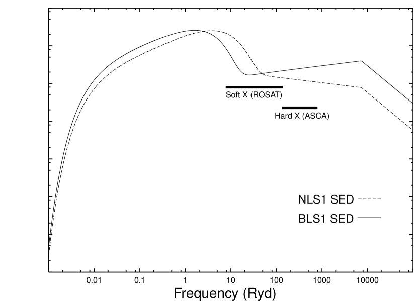
Figure 6.— The template SEDs adopted for the photoionization model cluculations. Arbitrary flux density (i.e., energy per unit frequency) in logarithmic scale is plotted as a function of frequency in the unit of Rydberg. The dashed curve is for NLS1s and the solid one is for BLS1s.

Here we construct the template SEDs of the NLS1 and the BLS1 taking the above observational properties into account. We adopt the following function for the templates:

$$f_{\nu}=\nu^{\alpha_{{\rm uv}}}\exp(-\frac{h\nu}{kT_{{\rm BB}}})\exp(-\frac{kT_{{\rm IR}}}{h\nu})+a\nu^{\alpha_{{\rm x}}}$$ (2)

(see Ferland 1996). We adopt the following parameter values. (I) $kT_{\rm IR}$ is the infrared cutoff of the so-called big blue bump component, and we fix $kT_{\rm IR}$ = 0.01 Ryd following to Ferland (1996). (II) $\alpha_{\rm UV}$ is the slope of the low-energy side of the big blue bump component. We adopt $\alpha_{\rm UV}$ = –0.5, which is the typical value for AGNs (Ferland 1996; see also Francis 1993). Note that the photoionization process is not sensitive to this parameter. (III) $\alpha_{\rm ox}$ is the UV–to–X-ray spectral slope mentioned above, which determines the parameter $a$ in the equation (2). We adopt $\alpha_{\rm ox}$ = –1.35, which is the average value for the sample of Walter & Fink (1993) mentioned above, for both sample. However, there are some claims that this parameter correlates to the X-ray spectral index (Walter & Fink 1993; Laor et al. 1994 Puchnarewicz et al. 1996), that is, $\alpha_{\rm ox}$ may be different between NLS1s and BLS1s. Hence we check the dependence of the calculation outputs on $\alpha_{\rm ox}$ in Section 4.3.3. (IV) $\alpha_{\rm x}$ is the slope of the X-ray component. We adopt $\alpha_{\rm x}$ = –1.15 for NLS1s and –0.85 for BLS1s corresponding to the observational results by $ASCA$ described in Section 4.1.1. This power-law component is not extrapolated below 1.36 eV or above 100 keV. Below 1.36 eV, this term is set to zero, while above 100 keV, the continuum is assumed to fall off as $\nu^{-3}$. And finally, (V) $T_{{\rm BB}}$ is the parameter which characterizes the shape of the big blue bump. We choose this parameter to reproduce the soft X-ray spectral index measured by ROSAT described in Section 4.1.1. It results in 1,180,000 K for NLS1s and 490,000 K for BLS1s. They correspond to $\Gamma_{\rm ROSAT}$ = 3.13 and 2.35, respectively. The template SEDs constructed in such a way are shown in Figure 6; hereafter we refer the NLS1 SED and the BLS1 SED, respectively.

It is notable that these template SEDs are not theoretically predicted ones, but the empirical ones. Although it has not been understood whether or not the soft excess component is well described by a blackbody, Pounds et al. (1994) mentioned that the soft excess can be characterized by a blackbody of $kT_{\rm BB}$ = 70 $\pm$ 10 eV [or $T_{\rm BB}=(8.1\pm 1.2)\times 10^{5}$ K]. This suggests that the temperature of our adopted SEDs is not too high. Puchnarewicz et al. (1996) also mentioned that the soft excess may be represented by thermal bremsstrahlung with $T_{\rm brem}$ = 10⁶ K. Mineshige et al. (2000) proposed a slim disk model whose maximum blackbody temperature is $kT_{\rm BB}\simeq 0.2(M_{\rm SMBH}/10^{5}M_{\odot})^{-1/4}$ keV [or $T_{\rm BB}\simeq 2.3\times 10^{6}(M_{\rm SMBH}/10^{5}M_{\odot})^{-1/4}$] for the soft excess of NLS1s where $M_{\rm SMBH}$ is the mass of a supermassive black hole. These studies are almost consistent with our empirical template SEDs.

4.2. The Calculation Procedure

We perform photoionization model calculations using the spectral synthesis code Cloudy version 90.04 (Ferland 1996), which solves the equations of statistical and thermal equilibrium and produces a self-consistent model of the run of temperature as a function of depth into the nebula. Here we assume an uniform density gas cloud with a plane-parallel geometry.

The parameters for the calculations are (1) the hydrogen density of the cloud ($n_{\rm H}$), (2) the ionization parameter ($U$), which is defined as the ratio of the ionizing photon density to the electron density, (3) the chemical compositions of the gas, and (4) the shape of the input SED. We perform several model runs covering the following ranges of parameters: 10³ cm${}^{-3}\leq n_{\rm H}\leq 10^{6}$ cm^-3 (and 10⁷ cm^-3 in Section 4.3.4) and 10${}^{-4}\leq U\leq 10^{-1}$. We set the gas-phase elemental abundance to be either solar or subsolar. The adopted solar abundances relative to hydrogen are taken from Grevesse & Anders (1989) with extensions by Grevesse & Noels (1993). The subsolar abundances are assumed that 90% of Mg, Si, and Fe, 50% of C and O, and 25% of N and S are locked into dust grains, as estimated for the Orion H ii region (e.g., Baldwin et al. 1991, 1996). For the input SEDs, we use the two types of SED: the NLS1 SED and the BLS1 SED, mentioned in the last section. The calculations are stopped when the temperature fall to 3000 K, below which gas does not contribute significantly to the optical emission lines.

4.3. The Results of the Calculations

4.3.1 Excitation

Figure 7.— The diagram of [O i]/[O iii]$\lambda$5007 versus [O ii]/[O iii]$\lambda$5007. The symbols are the same as in Figure 3. Our model calculations for the solar abundances are presented by dashed curves for the NLS1 SED and by solid curve for the BLS1 SED. The data points will move on the diagram as shown by the arrow if the extinction correlation of $A_{V}$ = 1.0 is applied.

Figure 8.— The diagram of [O iii]$\lambda$5007/H$\beta$ versus [N ii]/H$\alpha$. The model loci for the case of the solar abundances are the same as in Figure 7. Typical location of AGNs (see Figure 4 of Veilleux & Osterbrock 1987) on this diagram are shown by the box. The effect of the correction for the extinction is not shown in this figure because the reddening effect on these line ratios is negligiblly small.

Figure 9.— The diagram of [S ii]/[O iii]$\lambda$5007 versus [N ii]/[O iii]$\lambda$5007. The results of the model calculations for the case of the solar abundance are shown. The lines, the symbols, and the arrow are the same as in Figure 7.

Figure 10.— The diagram of [O i]/[O iii]$\lambda$5007 versus [O ii]/[O iii]$\lambda$5007. The results of the model calculations for the case of the subsolar abundance are shown. The lines, the symbols, and the arrow are the same as in Figure 7.

Figure 11.— The diagram of [S ii]/[O iii]$\lambda$5007 versus [N ii]/[O iii]$\lambda$5007. The results of the model calculations for the case of the subsolar abundance are shown. The lines, the symbols, and the arrow are the same as in Figure 7.

We show the results of the model calculations in the case of the solar abundances and compare them to the observations in Figure 7, which is a diagram of [O i]/[O iii]$\lambda$5007 versus [O ii]/[O iii]$\lambda$5007. This diagram has been used to discuss the physical properties of ionized gas traditionally (e.g., Heckman 1980; Baldwin, Phillips, & Terlevich 1981; Ferland & Netzer 1983; Evans et al. 1999). It is shown that there is a slight difference of [O i]/[O iii]$\lambda$5007 between the two model grids. The reason for this difference is thought as follows. The relative intensity of soft X-ray of NLS1s is stronger than that of BLS1s. This results in a larger partially ionized zone in NLRs of NLS1s. Since [O i] is selectively radiated from such partially ionized zone because its ionization potential is close to the ionization potential of hydrogen, NLS1s tend to exhibit stronger [O i]. However, the dispersion of the compiled data is larger than this difference. This means that the line ratios used in this diagram are insensitive to the difference of the shape of the template SEDs. This result is consistent with the previous work of Rodríguez-Ardila et al. (2000a). They presented their photoionization model calculations assuming two types of SEDs; i.e., the NLS1-like SED and the BLS1-like SED. As shown in Figure 7 of Rodríguez-Ardila et al. (2000a), the ratio of [O i]/[O iii]$\lambda$5007 is not so different between the model NLS1 and the model BLS1 (less than factor 3).

The comparison between the models and the observations shown in Figure 7 suggests $10^{4}{\rm cm}^{-3}\leq n_{\rm H}\leq 10^{5}{\rm cm}^{-3}$ and $10^{-3.5}\leq U\leq 10^{-3}$ for the NLRs of both samples. The estimated $U$ values seem to be rather lower than those calculated in some previous works (e.g., Ferland & Netzer 1983; Ho, Shields, & Filippenko 1993). In order to make it clear that this is not due to any selection effect of the samples, we show model grids on the diagram of [O iii]$\lambda$5007/H$\beta$ versus [N ii]/H$\alpha$, which is a familiar diagnostic diagram proposed by Veilleux & Osterbrock (1987), in Figure 8. Comparing this with Figure 4 of Veilleux & Osterbrock (1987), typical Seyferts are reproduced by the models with $10^{-3.5}\leq U\leq 10^{-3}$. This discrepancy between the result by us and by previous literature is thought to be partly because the following reason. The energy peak of the template SEDs in our models is at rather high energy than those in previous studies. Accordingly the relative amounts of photons whose energy is near the ionization potential of hydrogen increase. This leads to the lower $U$ because this parameter is defined using all photons which exceed the ionization potential of hydrogen although the photoionization is effective in the energy of near the ionization potential of hydrogen.

We investigate the gas properties with another diagnostic diagram: [S ii]/[O iii]$\lambda$5007 versus [N ii]/[O iii]$\lambda$5007 (Figure 9). It results in that the derived ranges in both $n_{\rm H}$ and $U$ are consistent with those obtained in Figure 7. There is very little difference between the model grids for NLS1s and those for BLS1s. It is notable that the scatter of the plotted data in this diagram is larger than that in Figure 6. This may be due to that the deblending H$\alpha$ from [N ii] is not be well done in some case if the spectral resolution is not so high. If this is the case, the flux measurement of H$\alpha$ may not also be well done. It means that it is dangerous to use traditional emission-line ratios such as [N ii]/H$\alpha$, [S ii]/H$\alpha$, and [O i]/H$\alpha$ for S1s. Alternatively, the scatter may reflect the variety of the nitrogen abundance because some previous works reported that some of Seyferts show evidences in favor of a nitrogen overabundance (Storchi-Bergmann & Pastoriza 1990; Storchi-Bergmann 1991; Storchi-Bergmann et al. 1998). In any case, the diagram of [S ii]/[O iii]$\lambda$5007 versus [N ii]/[O iii]$\lambda$5007 is less suitable to discuss the properties of gas in NLRs than that of [O i]/[O iii]$\lambda$5007 versus [O ii]/[O iii]$\lambda$5007.

In Figures 10 and 11, we show the result of the model calculations for the case of the subsolar abundances and compare them with the observations on the diagrams of [O i]/[O iii]$\lambda$5007 versus [O ii]/[O iii]$\lambda$5007 and [S ii]/[O iii]$\lambda$5007 versus [N ii]/[O iii]$\lambda$5007, respectively. The loci of model grids in Figure 10 slightly shift to be larger in [O i] than those in Figure 7. This may be attributed to the fact that the partially ionized region become thicker due to the decrease of the heavy elements. However, the estimated parameters, $n_{\rm H}$ and $U$, are almost the same as those in the case of the solar abundances.

4.3.2 [O iii] Emitting Region

Figure 12.— The diagram of [O iii]$\lambda$4363/[O iii]$\lambda$5007 versus [O i]/[O iii]$\lambda$5007. The results of the model calculations for the case of the solar abundance are shown. The lines, the symbols, and the arrow are the same as in Figure 7.

Figure 13.— The diagram of [O iii]$\lambda$4363/[O iii]$\lambda$5007 versus [O i]/[O iii]$\lambda$5007. The results of the model calculations for the case of the subsolar abundance are shown. The lines, the symbols, and the arrow are the same as in Figure 7.

Figure 14.— The gas temperature calculated with the models described in the text is shown as a function of the hydrogen column density from the surface of a cloud exposed to the ionizing source.

As mentioned in Section 3.2, the temperature-sensitive emission-line ratio, [O iii]$\lambda$4363/[O iii]$\lambda$5007, is scarcely different between the NLS1s and the BLS1s though the intrinsic SEDs are clearly different between them. In order to investigate whether or not this difference in SEDs causes a detectable difference in the temperature of NLR gas through photoionization processes, we carry out the model calculations concerning the [O iii]$\lambda$4363/[O iii]$\lambda$5007 ratio. In Figure 12, we show the diagram of [O iii]$\lambda$4363/[O iii]$\lambda$5007 versus [O i]/[O iii]$\lambda$5007 for the case of the solar abundances. It is shown that the very high density condition (10${}^{6}{\rm cm}^{-3}$ or higher) is needed to explain the observed [O iii]$\lambda$4363/[O iii]$\lambda$5007 ratios for both NLS1s and BLS1s. This derived $n_{\rm H}$ is far higher than the value obtained using the diagnostic diagrams presented in Section 4.3.1. The reason for this is partly because of the oversimplification of the photoionization models: the [O iii]$\lambda$4363/[O iii]$\lambda$5007 ratio is difficult to be reproduced by one-zone photoionization models as mentioned in other works (e.g., Filippenko & Halpern 1984; Tadhunter, Robinson, & Morganti 1989; Wilson, Binette, & Storchi-Bergmann 1997; Nagao, Murayama, & Taniguchi 2000a). We are not going to make further discussion for this problem because this is out of the purpose of this paper. In this diagram, the loci of the model grid for NLS1s slightly shift to be larger [O iii]$\lambda$4363/[O iii]$\lambda$5007 with respect to those for BLS1s, which means that the temperature of gas in NLRs of the model NLS1 is higher than that of the model BLS1. This is because the number of high energy photon is larger in NLS1s than in BLS1s (see Figure 6). However, it is evident that this difference of the model loci is much smaller than the dispersion of the observed data points. Therefore, we conclude that the difference of SEDs between the NLS1s and the BLS1s is not important when one investigates the [O iii]$\lambda$4363/[O iii]$\lambda$5007 ratio. As shown in Figure 13, almost the same results are obtained when the subsolar abundances are assumed on the model calculations.

In order to investigate the difference of gas temperature between NLS1s and BLS1s in more detail, we show the temperature structure in a cloud as a function of the hydrogen column density from the inner surface in Figure 14. Here we adopt $n_{\rm H}=10^{4.5}$ cm^-3 and $U=10^{-3}$ for the four model calculations. It is shown that the gas temperature in the case of the subsolar abundances is higher than the other, which is due to a decrease of coolant elements. Generally the temperature decreases as the column density increases. However, there is a small turn-up just before the ionization front where the temperature drops off. This is attributed to the fact that the most effective coolant, O²⁺, is exhausted at this region. It is important that the abundances more affect the temperature than the input SED. Therefore, the difference of SEDs between the NLS1s and BLS1s does not affect significantly the gas temperature proved by the [O iii] emission lines. This result is also consistent with Rodríguez-Ardila et al. (2000a), in which the ratio of [O iii]$\lambda$4363/[O iii]$\lambda$5007 is not so different between the model NLS1 and the model BLS1 (less than factor 3) though they suggested that the calculated ratio of [O iii]$\lambda$4363/[O iii]$\lambda$5007 is higher in the BLS1 than in the NLS1.

4.3.3 Dependence of the Calculation Results on $\alpha_{\rm ox}$

Figure 15.— The calculated line ratios of [O i]/[O iii]$\lambda$5007, [O ii]/[O iii]$\lambda$5007, and [O iii]$\lambda$4363/[O iii]$\lambda$5007 versus $\alpha_{\rm ox}$ for the NLS1 SED. The calculated line ratios for the BLS1 SED ($\alpha_{\rm ox}$ = –1.35) are plotted by squares. For the calculations, $n_{\rm H}=10^{4.5}$ cm^-3, $U=10^{-3}$ and solar abundances are assumed.

Figure 16.— The calculated gas temperature of a NLR gas of NLS1s for various $\alpha_{\rm ox}$ are shown by solid lines for the case of the NLS1 SED. The case of BLS1 SED ($\alpha_{\rm ox}$ = –1.35) is shown by dotted curve. For the calculations, $n_{\rm H}=10^{4.5}$ cm^-3, $U=10^{-3}$ and solar abundances are assumed.

As mentioned in Section 4.1, we have assumed that NLS1s and BLS1s have similar $\alpha_{\rm ox}$. However, there are some previous studies (Walter & Fink 1993; Laor et al. 1994; Puchnarewicz et al. 1996) in which it is claimed that the soft X-ray spectral index correlates with $\alpha_{\rm ox}$. Since the large X-ray spectral index is one of the characteristic properties of NLS1s, their claim means that NLS1s have the softer $\alpha_{\rm ox}$ than BLS1s, systematically. Therefore, we investigate the dependence of the calculations on $\alpha_{\rm ox}$.

When various values of $\alpha_{\rm ox}$ are adopted, $T_{\rm BB}$ must be correspondingly adjusted to reproduce the observed soft X-ray photon index, $\Gamma_{\rm ROSAT}$ = 3.13. We adopt $T_{\rm BB}$ = 980,000 K, 840,000 K, 730,000 K, 650,000 K, and 590,000 K for the cases of $\alpha_{\rm ox}$ = –1.40, –1.45, –1.50, –1.55, and –1.60, respectively.

In Figure 15, we show a diagram of calculated line ratios versus $\alpha_{\rm ox}$, adopting $n_{\rm H}=10^{4.5}$ cm^-3, $U=10^{-3}$, solar abundances, and the SED template of NLS1s. It is clearly shown that the [O II]/[O III]$\lambda$5007 ratio is almost independent of $\alpha_{\rm ox}$. On the other hand, the [O I]/[O III]$\lambda$5007 and the [O III]$\lambda$4363/[O III]$\lambda$5007 ratios become smaller and to be close to the value of BLS1s as $\alpha_{\rm ox}$ becomes softer. Thus, we conclude that the difference of intrinsic SEDs between NLS1s and BLS1s scarcely affects the NLR emission even if $\alpha_{\rm ox}$ of NLS1s is systematically softer than that of BLS1s.

In Figure 16, we show the temperature structure in a NLR cloud for various values of $\alpha_{\rm ox}$, adopting $n_{\rm H}=10^{4.5}$ cm^-3, $U=10^{-3}$, solar abundances, and the SED template of NLS1s. The gas temperature also becomes to be close to that of BLS1s as $\alpha_{\rm ox}$ becomes softer.

4.3.4 Highly Ionized Emission Lines

Figure 17.— The diagram of [Fe vii]$\lambda$6087/[O iii]$\lambda$5007 versus [O i]/[O iii]$\lambda$5007. The results of the model calculations for the case of solar abundances are shown. The lines, the symbols, and the arrow are te same as in Figure 7.

Figure 18.— The diagram of [Fe vii]$\lambda$6087/[O iii]$\lambda$5007 versus [O i]/[O iii]$\lambda$5007. The results of the model calculations for the case of subsolar abundances are shown. The lines, the symbols, and the arrow are te same as in Figure 7.

Seyfert galaxies often present highly ionized emission lines such as [Fe vii]$\lambda$6087, [Fe x]$\lambda$6374, [Fe xi]$\lambda$7892, and [Fe xiv]$\lambda$5303 (see Nagao et al. 2000c and references therein). These emission lines are useful to investigate the viewing angle toward dusty tori of Seyfert nuclei (Murayama & Taniguchi 1998a; Nagao et al. 2000c). Therefore it is important to investigate how the feature of intrinsic SEDs affects such highly ionized emission-line intensities.

We show the results of the model calculations for the case of the solar abundances and compare them with the observations in a diagram of [Fe vii]$\lambda$6087/[O iii]$\lambda$5007 versus [O i]/[O iii]$\lambda$5007 (Figure 17). The data of observations are taken from Nagao et al. (2000c). Being different from the results described in Section 4.3.1 and 4.3.2, there are evident differences in the behavior of the calculated line ratios between two models as follows. (1) The calculated [O i]/[O iii]$\lambda$5007 ratio for NLS1s is smaller than that for BLS1s when $U\sim 10^{-1}$ although the opposite trend is seen when $U<10^{-2}$. This is because the volume of the fully ionized region becomes larger with increasing ionization parameter, and thus the [O iii]$\lambda$5007 emission becomes more prominent relative to the [O i] emission. (2) The calculated [Fe vii]$\lambda$6087/[O iii]$\lambda$5007 ratio for NLS1s is several times larger than that for BLS1s when $U\leq 10^{-2}$. This is because the number of the high-energy ionizing photons producing Fe⁶⁺ in the model for NLS1s is much larger than that in the model for BLS1s when we adopt the same ionization parameter and the gas density for both cases.

However, clearly shown in Figure 17, the calculated [Fe vii]$\lambda$6087/[O iii]$\lambda$5007 is much smaller than the observed one in both models. This means that another component which radiates highly ionized emission lines is needed to explain the observations, which is consistent with previous studies (Stasińska 1984; Ferland & Osterbrock 1986; Binette et al. 1996; Murayama & Taniguchi 1998a, 1998b). Therefore this result does not suggest that the observed [Fe vii]$\lambda$6087/[O iii]$\lambda$5007 of NLS1s should be larger than that of BLS1s.

In Figure 18, we show the same diagram adopting the subsolar abundances. Similar to the case of the solar abundances, the calculated [Fe vii]$\lambda$6087/[O iii]$\lambda$5007 for BLS1s is smaller than that for NLS1s. In the case of the subsolar abundances, the large fraction of iron is depleted (see Section 4.2). Therefore, the calculated [Fe vii]$\lambda$6087/[O iii]$\lambda$5007 is much smaller than that calculated adopting the solar abundances.

5. CONCLUDING REMARKS

This paper has presented the comparisons of emission-line ratios which represent the ionization degree and the gas temperature of NLR clouds between the NLS1s and the BLS1s. The emission-line ratio of [O i]/[O iii]$\lambda$5007, which probes the ionization degree of NLRs, and that of [O iii]$\lambda$4363/[O iii]$\lambda$5007, which probes the gas temperature of NLRs, are indistinguishable between the two samples. This means that there is little difference in the physical properties of NLRs between NLS1s and BLS1s. Using photoionization models, we have confirmed that these results are consistent with the presence of differences in SEDs between NLS1s and BLS1s. In both cases, using the template SEDs of NLS1s and BLS1s, we have shown that the observed emission line ratios are well reproduced when we adopt $10^{4}{\rm cm}^{-3}\leq n_{\rm H}\leq 10^{5}{\rm cm}^{-3}$ and $10^{-3.5}\leq U\leq 10^{-3}$ for either solar or subsolar abundances.

This study tells us that we need not consider the effects of difference of intrinsic SEDs between NLS1s and BLS1s when we discuss ionized gas properties using diagnostic diagrams as used by, e.g., Ferland & Netzer (1983) and Ho et al. (1993), unless the high ionization nuclear emission-line region (Binette 1985; Murayama, Taniguchi, & Iwasawa 1998; Murayama & Taniguchi 1998a, 1998b; Nagao et al. 2000b, 2000c) is concerned.

Table 1The Properties of the Objects in Our Sample

Name	Another Name	Redshift	$\nu L_{\nu}$(60$\mu$m)	References for Emission Line Ratios
NLS1s
NGC 4051	$\cdots$	0.0024	2.348$\times$1010	M95, V88
NGC 4748	MCG -2-33-34, CTS R12.02	0.0146	1.419$\times$1011	W92, RPD00
Mrk 42	$\cdots$	0.0240	1.053$\times$1011	C91, K78, OP85
Mrk 291	$\cdots$	0.0352	2.428$\times$1011	O77
Mrk 335	PG 0003+199	0.0258	1.316$\times$1011	C94, O77, P78
Mrk 359	UGC 1032	0.0174	1.956$\times$1011	C94, DK78, OP85, V88
Mrk 478	PG 1440+356	0.0791	2.161$\times$1012	O77, P78
Mrk 493	UGC 10120	0.0319	4.099$\times$1011	C91, OP85
Mrk 504	PG 1659+294	0.0359	$\cdots$	O77
Mrk 507	$\cdots$	0.0559	1.010$\times$1012	K78
Mrk 739	NGC 3758	0.0299	6.499$\times$1011	C94, SO81
Mrk 766	NGC 4253	0.0129	3.830$\times$1011	C94, OP85, V88
Mrk 783	$\cdots$	0.0672	8.392$\times$1011	OP85
Mrk 896	$\cdots$	0.0264	2.068$\times$1011	C94, MW88
Mrk 957	5C 3.100	0.0711	6.390$\times$1012	K78
Mrk 1126	NGC 7450	0.0106	$\cdots$	OP85
Mrk 1239	$\cdots$	0.0199	3.038$\times$1011	C91, C94, OP85, RPD00
1E 1031+5822	$\cdots$	0.248	$\cdots$	S89
1E 1205+4657	$\cdots$	0.102	$\cdots$	S89
1E 12287+123	$\cdots$	0.116	$\cdots$	S89
2E 1226+1336	$\cdots$	0.150	$\cdots$	S89
2E 1557+2712	$\cdots$	0.0646	$\cdots$	S89
I Zw 1	UGC 545	0.0611	5.004$\times$1012	C94, O77, P78
Akn 564	UGC 12163	0.0247	2.901$\times$1011	C94, V88
CTS H34.06	IRAS F06083-5606	0.0318	1.396$\times$1011	RPD00
H 1934-063	IRAS 19348-0619	0.0106	1.787$\times$1011	RPD00
HE 1029-1831	CTS J04.08, IRAS 10295-1831	0.0403	2.413$\times$1012	RPD00
IRAS 15091-2107	$\cdots$	0.0446	1.777$\times$1012	W92
CTS J03.19	CTS 90	0.0532	$\cdots$	RPD00
CTS J13.12	CTS 103	0.0120	$\cdots$	RPD00
KAZ 163	VII Zw 742	0.0630	$\cdots$	S89
KAZ 320	$\cdots$	0.0345	$\cdots$	Z92
MS 01119-0132	$\cdots$	0.12	$\cdots$	S89
MS 01442-0055	$\cdots$	0.08	$\cdots$	S89
MS 12235+2522	$\cdots$	0.067	$\cdots$	S89
Q 0919+515	$\cdots$	0.161	$\cdots$	S89
BLS1s
NGC 4235	$\cdots$	0.0080	1.158$\times$1010	MW88, M95
NGC 4593	$\cdots$	0.0090	1.401$\times$1011	MW88
NGC 5940	$\cdots$	0.0337	4.915$\times$1011	MW88
Mrk 10	UGC 4013	0.0293	4.025$\times$1011	O77
Mrk 40	Arp 151	0.0211	$\cdots$	O77
Mrk 50	$\cdots$	0.0234	$\cdots$	MW88
Mrk 69	$\cdots$	0.0760	$\cdots$	O77
Mrk 79	UGC 3973	0.0222	4.250$\times$1011	C83, O77, V88
Mrk 106	$\cdots$	0.1235	$\cdots$	O77
Mrk 124	$\cdots$	0.0563	1.286$\times$1012	O77, P78
Mrk 141	$\cdots$	0.0417	7.533$\times$1011	O77
Mrk 142	PG 1022+519	0.0449	$\cdots$	O77, P78
Mrk 236	$\cdots$	0.0520	2.772$\times$1011	O77
Mrk 279	UGC 8823	0.0294	6.275$\times$1011	C83, O77
Mrk 304	II Zw 175, PG 2214+139	0.0658	$\cdots$	O77
Mrk 358	$\cdots$	0.0452	3.816$\times$1011	O77
Mrk 374	$\cdots$	0.0435	2.952$\times$1011	O77, P78
Mrk 382	$\cdots$	0.0338	1.431$\times$1011	O77
Mrk 486	PG 1535+547	0.0389	$\cdots$	O77, P78
Mrk 541	$\cdots$	0.0394	3.182$\times$1011	O77, P78
Mrk 590	NGC 863, UM 412	0.0264	1.965$\times$1011	O77
Mrk 618	$\cdots$	0.0356	1.990$\times$1012	O77, P78
Mrk 704	$\cdots$	0.0292	1.797$\times$1011	C83, C94, UW83
Mrk 705	UGC 5025	0.0292	2.900$\times$1011	C94
Mrk 876	PG 1613+658	0.1290	6.328$\times$1012	S89
Mrk 975	UGC 774	0.0496	1.163$\times$1012	C83, C94, V88
Mrk 1040	NGC 931	0.0167	4.047$\times$1011	C94, V88
Mrk 1044	PG 0157+001	0.0165	6.656$\times$1010	T91
Mrk 1347	$\cdots$	0.0497	1.337$\times$1012	MW88
1E 0514-0030	$\cdots$	0.292	$\cdots$	S89
1H 1836-786	IRAS F18389-7834	0.0743	1.246$\times$1012	MW88
1H 1927-516	CTS G03.04	0.0403	$\cdots$	RPD00
1H 2107-097	$\cdots$	0.0268	$\cdots$	W92, RPD00
2E 0150-1015	$\cdots$	0.361	$\cdots$	S89
2E 0237+3953	$\cdots$	0.528	$\cdots$	S89
2E 1401+0952	$\cdots$	0.441	$\cdots$	S89
2E 1530+1511	$\cdots$	0.090	$\cdots$	S89
2E 1556+2725	PGC 56527	0.0904	$\cdots$	S89
2E 1847+3329	$\cdots$	0.509	$\cdots$	S89
3C 263	$\cdots$	0.646	$\cdots$	P78
3C 382	CGCG 173-014	0.0579	$\cdots$	O77
III Zw 002	$\cdots$	0.0898	$\cdots$	O77
VII Zw 118	$\cdots$	0.0797	$\cdots$	C94, KS79
CTS A08.12	CTS 109	0.0293	$\cdots$	RPD00
AB 125	$\cdots$	0.281	$\cdots$	S89
Akn 120	UGC 3271	0.0323	3.891$\times$1011	P78, V88
Arp 102B	$\cdots$	0.0242	$\cdots$	SSK83
CTS B25.02	Tololo 0343-397	0.0432	2.622$\times$1011	T91
B2 1425+26	Ton 202, PG 1425+267	0.366	$\cdots$	P78
B2 1512+37	4C 37.43, PG 1512+370	0.3707	$\cdots$	P78
CTS C16.16	$\cdots$	0.0795	$\cdots$	RPD00
ESO 141-G55	$\cdots$	0.0360	4.335$\times$1011	MW88, W92
ESO 198-G24	$\cdots$	0.0455	$\cdots$	W92
ESO 323-G77	$\cdots$	0.0150	7.275$\times$1011	W92
ESO 438-G09	$\cdots$	0.0245	1.088$\times$1012	KF83
ESO 578-G09	CTS J14.05	0.0349	$\cdots$	RPD00
CTS F10.01	CTS 114	0.0784	$\cdots$	RPD00
Fairall 9	ESO 113-IG45	0.0470	$\cdots$	W92
Fairall 265	$\cdots$	0.0295	3.388$\times$1011	W92
Fairall 1116	Tololo 0349-406	0.0582	3.175$\times$1011	W92
Fairall 1146	$\cdots$	0.0316	$\cdots$	RPD00
CTS H34.03	IRAS F05561-5357	0.0967	2.769$\times$1012	RPD00
H 0557-385	CTS B31.01, IRAS F05563-3820	0.0344	$\cdots$	W92, RPD00
IC 4218	$\cdots$	0.0194	$\cdots$	MW88
IC 4329A	$\cdots$	0.0161	2.987$\times$1011	MW88, W92, WP79
CTS J10.09	IRAS F12312-2047	0.0230	1.164$\times$1011	RPD00
CTS M02.30	IRAS F10306-2651	0.0688	7.266$\times$1011	RPD00
MC 1104+167	4C 16.30	0.632	$\cdots$	P78
MS 02255+3121	$\cdots$	0.058	$\cdots$	S89
MS 07451+5545	$\cdots$	0.174	$\cdots$	S89
MS 08451+3751	$\cdots$	0.307	$\cdots$	S89
MS 08495+0805	$\cdots$	0.062	$\cdots$	S89
MS 10590+7302	$\cdots$	0.089	$\cdots$	S89
MS 11397+1040	$\cdots$	0.150	$\cdots$	S89
MS 13396+0519	$\cdots$	0.266	$\cdots$	S89
MS 13575-0227	$\cdots$	0.416	$\cdots$	S89
MS 15251+1551	$\cdots$	0.230	$\cdots$	S89
MS 22152-0347	$\cdots$	0.242	$\cdots$	S89
PG 1352+183	$\cdots$	0.152	$\cdots$	S89
PKS 1417-19	CTS J15.22, CTS 105	0.120	$\cdots$	RPD00
Tololo 20	$\cdots$	0.030	$\cdots$	MW88
Ton 1542	PG 1229+204	0.0640	$\cdots$	P78
Zw 0033+45	CGCG 535-012	0.0476	$\cdots$	C94

Table 2Compiled Emission-Line Flux Ratios

Name	[O i]/[O iii]$\lambda$5007	[O ii]/[O iii]$\lambda$5007	[O iii]$\lambda$4363/[O iii]$\lambda$5007	[N ii]/[O iii]$\lambda$5007	[S ii]/[O iii]$\lambda$5007
NLS1s
NGC 4051	0.1300	$\cdots$	$\cdots$	1.0190	0.3160
NGC 4748	0.0400	0.1883	0.0492	0.3000	0.2100
Mrk 42	0.1435	0.3696	0.1339	1.8248	0.5680
Mrk 291	0.1031	0.4742	0.1031	1.1031	0.4845
Mrk 335	0.0667	0.4316	0.0699	$<$ 1.4783	0.0571
Mrk 359	0.0577	0.1790	0.0735	0.2120	0.1297
Mrk 478	0.0740	0.4280	$\cdots$	$\cdots$	0.2040
Mrk 493	$\cdots$	0.5600	0.4568	2.0400	0.8240
Mrk 504	$\cdots$	$\cdots$	0.0308	$\cdots$	0.1192
Mrk 507	0.2099	0.5679	0.0593	4.3951	1.1481
Mrk 739	0.3700	0.8894	$<$ 0.0740	4.2800	2.1500
Mrk 766	0.0241	0.0763	0.0294	0.2166	0.0695
Mrk 783	0.0584	0.2957	0.0895	0.1479	0.1479
Mrk 896	$\cdots$	0.5276	$\cdots$	$\cdots$	0.1626
Mrk 957	0.3016	0.8730	0.0952	3.4444	1.1111
Mrk 1126	0.0791	0.1279	0.1163	5.8140	0.3233
Mrk 1239	0.0200	0.0852	0.0892	0.3011	0.1128
1E 1031+5822	1.1280	0.7082	0.0683	$\cdots$	$\cdots$
1E 1205+4657	0.0555	$\cdots$	0.3646	$\cdots$	0.7376
1E 12287+123	$\cdots$	$\cdots$	0.5395	$\cdots$	0.6974
2E 1226+1336	$\cdots$	0.3493	0.0312	$\cdots$	0.4521
2E 1557+2712	$\cdots$	$\cdots$	$\cdots$	$\cdots$	0.6269
I Zw 1	0.0636	0.4756	0.0761	$\cdots$	0.0295
Akn 564	$\cdots$	0.4068	$\cdots$	$\cdots$	$\cdots$
CTS H34.06	$\cdots$	0.3421	0.1023	$\cdots$	$\cdots$
H 1934-063	$\cdots$	0.1257	0.0437	$\cdots$	$\cdots$
HE 1029-1831	$\cdots$	0.1961	0.0980	$\cdots$	$\cdots$
IRAS 15091-2107	$\cdots$	0.1400	0.0500	0.3200	0.3600
CTS J03.19	$\cdots$	0.1626	$\cdots$	$\cdots$	$\cdots$
CTS J13.12	$\cdots$	$\cdots$	0.3101	$\cdots$	$\cdots$
KAZ 163	$\cdots$	$\cdots$	$\cdots$	$\cdots$	0.1418
KAZ 320	0.0629	0.3452	0.0595	0.2151	0.2738
MS 01119-0132	$\cdots$	$\cdots$	0.1188	$\cdots$	$\cdots$
MS 01442-0055	$\cdots$	$\cdots$	0.0207	$\cdots$	0.2434
MS 12235+2522	$\cdots$	$\cdots$	$\cdots$	$\cdots$	0.2120
Q 0919+515	$\cdots$	0.2191	$\cdots$	$\cdots$	$\cdots$
BLS1s
NGC 4235	0.1967	0.6389	0.2837	0.6610	0.6252
NGC 4593	0.0470	0.1696	$\cdots$	$\cdots$	0.1357
NGC 5940	0.0772	$\cdots$	$\cdots$	$\cdots$	0.1680
Mrk 10	0.0172	0.0871	0.0247	0.1183	0.0763
Mrk 40	0.1111	0.5000	0.1667	0.2639	0.1444
Mrk 50	0.1218	0.3261	$\cdots$	$\cdots$	0.1851
Mrk 69	$\cdots$	0.4186	0.0837	1.0698	0.3512
Mrk 79	0.0424	0.1763	0.0457	0.2591	0.1741
Mrk 106	0.0414	0.2000	0.0310	0.2241	$\cdots$
Mrk 124	0.0628	0.3577	0.0730	$\cdots$	0.2394
Mrk 141	$\cdots$	0.1632	0.0816	0.9474	0.3763
Mrk 142	$<$ 0.0857	0.3760	0.0680	1.3200	0.5669
Mrk 236	0.0717	0.1848	0.0804	0.1587	0.2565
Mrk 279	0.1312	0.4635	0.0670	0.6483	0.3204
Mrk 304	$<$ 0.0455	0.1212	0.1061	0.3788	0.1818
Mrk 358	$<$ 0.0977	0.2326	$<$ 0.0605	0.3256	0.3953
Mrk 374	0.0686	0.0914	0.0738	0.0628	0.1188
Mrk 382	$\cdots$	0.0805	0.0322	0.3333	0.7805
Mrk 486	0.0917	$<$ 0.1500	$\cdots$	$\cdots$	0.0773
Mrk 541	$<$ 0.2050	0.1739	0.2217	1.3755	0.5600
Mrk 590	0.2000	0.2182	0.2000	0.5455	0.2345
Mrk 618	0.0549	0.1356	0.0410	0.8667	0.2320
Mrk 704	0.0287	0.2016	0.0726	0.1710	0.1507
Mrk 705	$\cdots$	0.1532	$\cdots$	$\cdots$	$\cdots$
Mrk 876	0.1659	$\cdots$	0.0272	$\cdots$	0.7093
Mrk 975	0.0248	0.1998	0.0303	0.4421	0.0634
Mrk 1040	$\cdots$	0.0850	$\cdots$	$\cdots$	$\cdots$
Mrk 1044	$\cdots$	0.1238	$\cdots$	$\cdots$	$\cdots$
Mrk 1347	$\cdots$	0.6032	$\cdots$	$\cdots$	0.2063
1E 0514-0030	$\cdots$	$\cdots$	0.4949	$\cdots$	$\cdots$
1H 1836-786	0.0349	0.1623	$\cdots$	$\cdots$	0.1623
1H 1927-516	$\cdots$	$\cdots$	0.0792	$\cdots$	$\cdots$
1H 2107-097	0.1300	0.1300	0.1696	$\cdots$	$\cdots$
2E 0150-1015	$\cdots$	0.1291	0.0341	$\cdots$	$\cdots$
2E 0237+3953	$\cdots$	0.3364	0.0757	$\cdots$	$\cdots$
2E 1401+0952	$\cdots$	$\cdots$	0.0565	$\cdots$	$\cdots$
2E 1530+1511	$\cdots$	$\cdots$	$\cdots$	$\cdots$	0.2091
2E 1556+2725	0.0430	$\cdots$	0.0884	$\cdots$	0.2033
2E 1847+3329	$\cdots$	0.1800	0.0649	$\cdots$	$\cdots$
3C 263	$\cdots$	$\cdots$	0.0515	$\cdots$	$\cdots$
3C 382	0.0700	0.1300	0.1600	0.0400	0.1600
III Zw 002	0.0576	0.1394	0.0273	0.1333	0.1576
VII Zw 118	$\cdots$	0.4444	$\cdots$	$\cdots$	$\cdots$
CTS A08.12	$\cdots$	0.1280	0.0759	$\cdots$	$\cdots$
AB 125	$\cdots$	0.2922	$\cdots$	$\cdots$	$\cdots$
Akn 120	0.0917	0.2658	$\cdots$	$\cdots$	0.3108
Arp 102B	0.8030	1.1970	0.0571	1.9343	1.2475
CTS B25.02	$\cdots$	0.3207	$\cdots$	$\cdots$	$\cdots$
B2 1425+26	$\cdots$	$\cdots$	0.0417	$\cdots$	$\cdots$
B2 1512+37	$\cdots$	$\cdots$	0.0393	$\cdots$	$\cdots$
CTS C16.16	$\cdots$	0.1793	0.0588	$\cdots$	$\cdots$
ESO 141-G55	$\cdots$	0.0924	$\cdots$	$\cdots$	0.2800
ESO 198-G24	$\cdots$	0.2700	$\cdots$	$\cdots$	0.1300
ESO 323-G77	$\cdots$	0.1300	$\cdots$	$\cdots$	0.2400
ESO 438-G09	0.0811	0.4324	0.0541	1.0000	0.4595
ESO 578-G09	$\cdots$	0.1719	0.0898	$\cdots$	$\cdots$
CTS F10.01	$\cdots$	0.1048	0.0391	$\cdots$	$\cdots$
Fairall 9	$\cdots$	0.0800	0.1200	0.2000	$\cdots$
Fairall 265	$\cdots$	0.7600	$\cdots$	1.3500	$\cdots$
Fairall 1116	$\cdots$	0.2000	0.0900	$\cdots$	0.5400
Fairall 1146	$\cdots$	0.1570	0.0436	$\cdots$	$\cdots$
CTS H34.03	$\cdots$	$\cdots$	0.1287	$\cdots$	$\cdots$
H 0557-385	$\cdots$	0.0816	$\cdots$	$\cdots$	0.1200
IC 4218	$\cdots$	0.2318	$\cdots$	$\cdots$	0.1706
IC 4329A	0.0964	0.0429	$\cdots$	0.3091	0.3156
CTS J10.09	$\cdots$	0.1034	0.1565	$\cdots$	$\cdots$
CTS M02.30	$\cdots$	0.1597	0.1875	$\cdots$	$\cdots$
MC 1104+167	$\cdots$	$\cdots$	0.0941	$\cdots$	$\cdots$
MS 02255+3121	$\cdots$	$\cdots$	0.1270	$\cdots$	$\cdots$
MS 07451+5545	$\cdots$	0.2066	0.0337	$\cdots$	$\cdots$
MS 08451+3751	$\cdots$	$\cdots$	0.1198	$\cdots$	$\cdots$
MS 08495+0805	0.0313	$\cdots$	0.0395	$\cdots$	0.1261
MS 10590+7302	$\cdots$	$\cdots$	$\cdots$	$\cdots$	0.1080
MS 11397+1040	$\cdots$	$\cdots$	0.0215	$\cdots$	0.1304
MS 13396+0519	$\cdots$	0.5666	$\cdots$	$\cdots$	$\cdots$
MS 13575-0227	$\cdots$	0.1029	$\cdots$	$\cdots$	$\cdots$
MS 15251+1551	$\cdots$	0.0675	0.0405	$\cdots$	$\cdots$
MS 22152-0347	$\cdots$	0.1071	0.0329	$\cdots$	$\cdots$
PG 1352+183	$\cdots$	$\cdots$	$\cdots$	$\cdots$	0.2090
PKS 1417-19	$\cdots$	$\cdots$	0.1039	$\cdots$	$\cdots$
Tololo 20	0.0425	0.0800	0.0924	$\cdots$	0.0337
Ton 1542	$\cdots$	0.1944	0.1167	$\cdots$	0.1333
Zw 0033+45	0.2727	$\cdots$	$\cdots$	$\cdots$	$\cdots$

References

- (1)
- (2) Antonucci, R. R. J. 1993, ARA&A, 31, 473
- (3) Antonucci, R. R. J., & Miller, J. S. 1985, ApJ, 297, 621
- (4) Baldwin, J. A., et al. 1996, ApJ, 468, L115
- (5) Baldwin, J. A., Ferland, G. J., Martin, P. G., Corbin, M. R., Cota, S. A., Peterson, B. M., & Slettebak, A. 1991, ApJ, 374, 580
- (6) Baldwin, J. A., Phillips, M. M., & Terlevich, R. 1981, PASP, 93, 5
- (7) Binette, L. 1985, A&A, 143, 334
- (8) Binette, L., Wilson, A. S., & Storchi-Bergmann, T. 1996, A&A, 312, 365
- (9) Boller, T., Brandt, W. N., & Fink, H. 1996, A&A, 305, 53
- (10) Brandt, W. N., Mathur, S., & Elvis, M. 1997, MNRAS, 285, L25
- (11) Cardelli, J. A., Clayton, G. C., & Mathis, J. S. 1989, ApJ, 345,245
- (12) Cohen, R. D. 1983, ApJ, 273, 489
- (13) Contini, M., & Aldrovandi, S. M. V. 1983, A&A, 127, 15
- (14) Crenshaw, D. M., Peterson, B. M., Korista, K. T., Wagner, R. M., & Aufdenberg, J. P. 1991, AJ, 101, 1202
- (15) Cruz-González, I., Carrasco, L., Serrano, A., Guichard, J., Dultzin-Hacyan, D., & Bisiacchi, G. F. 1994, ApJS, 94, 47
- (16) Cruz-González, I., Guichard, J., Serrano, A., & Carrasco, L. 1991, PASP, 103, 888
- (17) Dahari, O., & De Robertis, M. M. 1988a, ApJS, 67, 249
- (18) Dahari, O., & De Robertis, M. M. 1988b, ApJ, 331, 727
- (19) Davidson, K., & Kinman, T. D. 1978, ApJ, 225, 776
- (20) De Zotti, G., & Gaskell, C. M. 1985, A&A, 147, 1
- (21) Dopita, M. A., & Sutherland, R. S. 1995, ApJ, 455, 468
- (22) Efstathiou, A., & Rowan-Robinson, M. 1995, MNRAS, 273, 649
- (23) Evans, I., Koratkar, A., Allen, M., Dopita, M., & Tsvetanov, Z. 1999, ApJ, 521, 531
- (24) Fadda, D., Giuricin, G., Granato, G., & Vecchies, D. 1998, ApJ, 496, 117
- (25) Ferland, G. J. 1996, Hazy: A Brief Introduction to Cloudy (Lexington: Univ. Kentucky Dept. Phys. Astron.)
- (26) Ferland, G. J., & Netzer, H. 1983, ApJ, 264, 105
- (27) Ferland, G. J., & Osterbrock, D. E. 1986, ApJ, 300,658
- (28) Fillippenko, A. V., Halpern, J. P. 1984, ApJ, 285, 458
- (29) Francis, P. J. 1993, ApJ, 407, 519
- (30) Grevesse, N., & Anders. E. 1989, in AIP Conf. Proc. 183, Cosmic Abundance of Matter, ed. Waddington, C. J. (New York: AIP), 1
- (31) Grevesse, N., & Noels, A. 1993, in Orisin & Evolution of the Elements, ed. Prantzos, N., Vangioni-Flam, E., & Casse, M. (Cambridge Univ. Press), 15
- (32) Heckman, T. M. 1980, A&A, 87, 152
- (33) Heckman, T. M., & Balick, B. 1979, A&A, 79, 350
- (34) Ho, L., Shields, J. C., & Filippenko, A. V. 1993, ApJ, 410, 567
- (35) Khachikian, E. Ye., & Weedman, D. W. 1974, ApJ, 192, 581
- (36) Kollatschny, W., & Fricke, K. J. 1983, A&A, 125, 276
- (37) Koski, A. T. 1978, ApJ, 223, 56
- (38) Kunth, D., & Sargent, W. L. W. 1979, A&A, 76, 50
- (39) Laor, A., Fiore, F., Elvis, M., Wilkes, B. J., & McDowell, J. C. 1994, ApJ, 435, 611
- (40) Leighly, K. M. 1999a, ApJS, 125, 297
- (41) Leighly, K. M. 1999b, ApJS, 125, 317
- (42) Mineshige, S., Kawaguchi, T., Takeuchi, M., & Hayashida, K. 2000, PASJ, in press (astro-ph/0003017)
- (43) Morris, S. L., & Ward, M. J. 1988, MNRAS, 230, 639
- (44) Moshir, M., et al. 1992, Explanatory Supplement to the IRAS Faint Source Survey (Version 2, JPL-D-10015 8/92; Pasadena: JPL)
- (45) Murayama, T. 1995, Master’s thesis, Tohoku Univ.
- (46) Murayama, T., Nagao, T., & Taniguchi, Y. 1999, Observational and Theoretical Progress in the Study of Narrow-Line Seyfert 1 Galaxies, ed. Boller, T. in press (astro-ph/0005138)
- (47) Murayama, T., & Taniguchi, Y. 1998a, ApJ, 497, L9
- (48) Murayama, T., & Taniguchi, Y. 1998b, ApJ, 503, L115
- (49) Murayama, T., & Taniguchi, Y., & Iwasawa, K. 1998, AJ, 115, 460
- (50) Nagao, T., Murayama, T., & Taniguchi, Y. 2000a, ApJ, submitted
- (51) Nagao, T., Murayama, T., Taniguchi, Y., & Yoshida, M. 2000b, AJ, 119, 620
- (52) Nagao, T., Taniguchi, Y., & Murayama, T. 2000c, AJ, 119, 2605
- (53) Netzer, H., & Laor, A. 1993, ApJ, 404, L51
- (54) Osterbrock, D. E. 1977, ApJ, 215, 733
- (55) Osterbrock, D. E. 1989, Astrophysics of Gaseous Nebulae and Active Galactic Nuclei (University Science Books)
- (56) Osterbrock, D. E. 1993, ApJ, 404, 551
- (57) Osterbrock, D. E., & Pogge, R. W. 1985, ApJ, 297, 166
- (58) Phillips, M. M. 1978, ApJ, 226, 736
- (59) Pier, E. A., & Krolik, J. H. 1992, ApJ, 401, 99
- (60) Pounds, K. A., Nandra, K., Fink, H. H., & Makino, F. 1994, MNRAS, 267, 193
- (61) Press, W. H., Teukolsky, S. A., Vetterling, W. T., & Flannery, B. P. 1988, Numerical Recipes in C (Cambridge University Press)
- (62) Puchnarewicz, E. M., Mason, K. O., Córdova, F. A., Kartje, J., Branduardi-Raymont, G., Mittaz, J. P. D., Murdin, P. G., & Allington-Smith, J. 1992, MNRAS, 256, 589
- (63) Puchnarewicz, E. M., Mason, K. O., Romero-Colmenero, E., Carrera, F. J., Hasinger, G., McMahon, R., Mittaz, J. P. D., Page, M. J., & Carballo, R. 1996, MNRAS, 281, 1243
- (64) Rodríguez-Ardila, A., Binette, L., Pastoriza, M. G., & Donzelli, C. J. 2000a, ApJ, in press (astro-ph/0003287)
- (65) Rodríguez-Ardila, A., Pastoriza, M. G., & Donzelli, C. J. 2000b, ApJS, 126, 63
- (66) Rodríguez-Pascual, P. M., Mas-Hesse, J. M., & Santos-Lleó, M. 1997, A&A, 327, 72
- (67) Shuder, J. M. 1981, ApJ, 244, 12
- (68) Shuder, J. M., & Osterbrock, D. E. 1981, ApJ, 250, 55
- (69) Stasińska, G. 1984, A&A, 135, 341
- (70) Stauffer, J., Schild, R., & Keel, W. 1983, ApJ, 270, 465
- (71) Stephens, S. A. 1989, AJ, 97, 10
- (72) Storchi-Bergmann, T. 1991, MNRAS, 249, 404
- (73) Storchi-Bergmann, T., Mulchaey, J. S., & Wilson, A. S. 1992, ApJ, 395, L73
- (74) Storchi-Bergmann, T., Pastoriza, M. G. 1990, PASP, 102, 1359
- (75) Storchi-Bergmann, T., Schmitt, H. R., Calzetti, D. & Kinney, A. L. 1998, AJ, 115, 909
- (76) Tadhunter, C. N., Robinson, A., & Morganti, R. 1989, in ESO Workshop on Extranuclear Activity in Galaxies, ed. Meurs, E. J. A., & Fosbury, R. A. E. (Garching: ESO), 293
- (77) Tananbaum, H., et al. 1979, ApJ, 234, L9
- (78) Taniguchi, Y., Murayama, T., & Nagao, T. 1999, ApJ, submitted (astro-ph/9910036)
- (79) Terlevich, R., Melnick, J., Masegosa, J., Moles, M., & Copetti, M. V. F. 1991, A&AS, 91, 285
- (80) Turner, T. J., George, I. M., Nandra, K., & Turcan, D. 1999, ApJ, 524, 667
- (81) Ulvestad, J. S., & Wilson, A. S. 1983, AJ, 88, 253
- (82) Vaughan, S., Reeves, J., Warwick, R., & Edelson, R. 1999, MNRAS, 309, 113
- (83) Veilleux, S. 1988, AJ, 95, 1695
- (84) Veilleux, S., & Osterbrock, D. E. 1987, ApJS, 63, 295
- (85) Viegas-Aldrovandi, S. M., & Contini, M. 1989, A&A, 215, 253
- (86) Walter, R., & Fink, H. H. 1993, A&A, 274, 105
- (87) Wang, T., Brinkmann, W., & Bergeron, J. 1996, A&A, 309, 81
- (88) Wilson, A. S., & Penston, M. V. 1979, ApJ, 232, 389
- (89) Wilson, A. S., Binette, L., & Storchi-Bergmann, T. 1997, ApJ, 482, L131
- (90) Winkler, H. 1992, MNRAS, 257, 677
- (91) Yee, H. K. C. 1980, ApJ, 241, 894
- (92) Zamorani, G., et al. 1981, ApJ, 245, 357
- (93) Zamorano, J., Gallego, J., Rego, M., Vitores, A. G., & Gonzalez-Riestra, R. 1992, AJ, 104, 1000
- (94)