A Global Photometric Analysis of 2MASS Calibration Data

Abstract

We present results from the application of a global photometric calibration (GPC) procedure to calibration data from the first 2 years of The Two Micron All Sky Survey (2MASS). The GPC algorithm uses photometry of both primary standards and moderately bright ‘tracer’ stars in 35 2MASS calibration fields. During the first two years of the Survey, each standard was observed on approximately 50 nights, with about 900 individual measurements. Based on the photometry of primary standard stars and secondary tracer stars and under the assumption that the nightly zeropoint drift is linear, GPC ties together all calibration fields and all survey nights simultaneously, producing a globally optimized solution. Calibration solutions for the Northern and Southern hemisphere observatories are found separately, and are tested for global consistency based on common fields near the celestial equator.

Several results from the GPC are presented, including establishing candidate secondary standards, monitoring of near-infrared atmospheric extinction coefficients, and verification of global validity of the standards. The solution gives long-term averages of the atmospheric extinction coefficients, $A_{J}=0.096$, $A_{H}=0.026$, $A_{K_{s}}=0.066$ (North) and $A_{J}=0.092$, $A_{H}=0.031$, $A_{K_{s}}=0.065$ (South), with formal error of $0.001$. The residuals show small seasonal variations, most likely due to changing atmospheric content of water vapor. Extension of the GPC to $\sim 100$ field stars in each of the 35 calibration fields yields a catalog of more than two thousand photometric standards ranging from $10^{th}$ to $14^{th}$ magnitude, with photometry that is globally consistent to $\sim 1\%$.

1 Introduction

The Two Micron All Sky Survey (2MASS) maps the entire sky in three near-infrared (NIR) bands, $J$ ($1.25\mu$m), $H$ ($1.65\mu$m), and $K_{s}$ ($2.16\mu$m). The survey operates in both hemispheres, with the Northern facility at Mt. Hopkins, AZ and the Southern site at Cerro Tololo, Chile. Both sites acquire data with nearly identical $1.3$ m cassegrain equatorial telescopes optimized for efficient sky coverage. Each telescope is equipped with three NICMOS3 arrays capable of simultaneous observations in three NIR bands. The Northern 2MASS facility began routine survey observations in June 1997, while the Southern facility started in March 1998.

Nightly photometric calibration for 2MASS is derived using repeated observations of $1^{\circ}\times 8.5^{\prime}$ calibration “fields” (see Table 1). Each hour, one of 40 calibration fields is scanned six times in the normal survey mode, providing six independent measurements of the standard stars in each field. The 2MASS calibration fields were selected initially to contain at least one “primary” calibration star drawn from the list of faint infrared standards published by Persson et al. (1998) and Casali & Hawarden (1992). One of the fields, 92049, does not contain an a priori standard star, but was selected to fill a gap in the right ascension coverage of the fields. Photometry for the calibration stars in this field was developed using the techniques described in §3.1 of this work. Table 1 contains a listing of the 2MASS calibration fields and the a priori catalog magnitudes for the primary calibration stars in each. The fields centers listed are the coordinates of the primary calibration stars. The analysis described in this paper uses 2MASS pipeline source extractions and photometry from repeated observations of 35 of the calibration fields.

Table 1: 2MASS calibration fields. Each field is $8.5^{\prime}\times 1^{\circ}$, centered on given coordinates of the fiducial standard. The equatorial fields are observed by both 2MASS facilities in the course of the survey to ensure uniformity between hemispheres. The listed magnitudes are the ones contained in the literature.

Number	Name	R.A. (J2000.0)	Dec. (J2000.0)	$J$	$H$	$K_{s}$	$N_{src}$
Zenith (North):
90091a	P091-D	$09:42:58.7$	$+59:03:43$	11.676	11.348	11.276	76
90182a	P182-E	$18:39:33.8$	$+49:05:38$	12.106	11.774	11.701	253
90161a	P161-D	$07:00:52.0$	$+48:29:24$	11.695	11.418	11.369	192
90290a	P290-D	$23:30:33.5$	$+38:18:57$	11.641	11.362	11.281	204
90247a	P247-U	$03:32:03.0$	$+37:20:39$	11.952	11.626	11.530	394
90272a	P272-D	$14:58:33.2$	$+37:08:33$	11.632	11.284	11.214	74
90266a	P266-C	$12:14:25.4$	$+35:35:56$	11.631	11.370	11.322	66
90330a	P330-E	$16:31:33.6$	$+30:08:48$	11.811	11.489	11.430	126
92409e	Abell2409	$22:00:28.0$	$+20:51:00$	—	—	—	252
Equatorial:
90067b	M67	$08:51:14.1$	$+11:50:52$	13.013	12.724	12.662	425
90533a	P533-D	$03:41:02.4$	$+06:56:13$	11.750	11.430	11.353	111
90565a	P565-C	$16:26:42.7$	$+05:52:20$	12.171	11.903	11.840	189
90191c	LHS191	$04:26:20.6$	$+03:37:25$	11.620	11.038	10.699	150
90004b	FS4	$01:54:37.8$	$+00:43:02$	10.573	10.328	10.294	83
90893a	S893-D	$23:18:10.1$	$+00:32:55$	11.403	11.123	11.063	86
90013b	FS13	$05:57:07.6$	$+00:01:11$	10.524	10.201	10.149	374
90860a	S860-D	$12:21:39.4$	$-00:07:13$	12.190	11.905	11.852	66
90867a	S867-V	$14:40:58.0$	$-00:27:47$	12.023	11.681	11.610	99
90868c	T868-53850	$15:00:26.4$	$-00:39:28$	11.595	10.991	10.641	113
92026c	LHS2026	$08:32:30.0$	$-01:34:14$	12.078	11.485	11.149	206
90021c	BRI0021-0214	$00:24:24.6$	$-01:58:22$	11.864	11.074	10.561	81
90547c,d	L547	$18:51:17.9$	$-04:16:28$	11.872	9.831	8.870	7302
90808a	S808-C	$19:01:55.5$	$-04:29:12$	10.936	10.620	10.545	3575
90813a	S813-D	$20:41:05.2$	$-05:03:43$	11.473	11.137	11.077	276
92202c	BRI2202-1119	$22:05:35.8$	$-11:04:29$	11.666	11.077	10.736	117
92397c	LHS2397a	$11:21:49.1$	$-13:13:13$	11.897	11.190	10.709	100
Zenith (South):
90009c	Oph-n9a	$16:27:13.2$	$-24:41:23$	15.381	12.278	10.733	244
90312a	S312-T	$08:25:36.2$	$-39:05:58$	11.949	11.669	11.609	1358
90294a	S294-D	$00:33:15.3$	$-39:24:10$	10.914	10.637	10.582	65
90301a	S301-D	$03:26:53.9$	$-39:50:38$	12.153	11.842	11.788	87
90273a	S273-E	$14:56:52.0$	$-44:49:14$	11.301	10.896	10.850	661
90279a	S279-F	$17:48:22.7$	$-45:25:45$	12.457	12.124	12.034	1846
90234a	S234-E	$20:31:20.5$	$-49:38:59$	12.464	12.127	12.070	187
90217a	S217-D	$12:01:45.2$	$-50:03:10$	11.294	11.000	10.923	595
90121a	S121-E	$06:29:29.4$	$-59:39:31$	12.114	11.838	11.781	207

^aNICMOS Standards (Persson et al. 1998);

^bUKIRT Faint Standards (Casali & Hawarden 1992);

^cFaint Red Standards (Persson et al. 1998);

^dBased on 2MASS observations, red standard L547 was found variable and was subsequently replaced by another star, selected from secondary standards, see §3.1.

^eInternal calibration field defined by the 2MASS Project; contains no fiducial standard.

The paper has three major parts: §2, which introduces the global photometric calibration method and compares it to nightly calibration; §3, which presents the results of major applications of the procedure to 2MASS data; and §4, which restates and summarizes the main results of the analysis. The major applications of GPC are: (i) establishment of secondary standards (§3.1), (ii) study of atmospheric extinction in near-infrared (§3.2), and (iii) analysis of global consistency (§3.3). Technical aspects of the method are given in Appendix A.

2 Global Photometric Calibration (GPC)

The purpose of nightly photometric calibration is to transfer instrumental magnitudes, $m_{inst}$, onto a uniform photometric system $m_{cal}$:

$$m_{cal}=m_{inst}+C_{1}-C_{2}\,(X-1),$$ (1)

where $C_{1}$ is the photometric zero point, $C_{2}$ is the atmospheric extinction correction, and $X$ is the airmass. Figure 1 plots a typical night of calibration data, showing both the data points (photometry of primary standards) and the nightly calibration solution $C_{1}$ (straight line). Each cluster of points in the nightly calibration plot is derived from one set of calibration observations. Each cluster consists of six data points which plot the zeropoint offset (i.e., $m_{cal}-m_{inst}+C_{2}\,(X-1)$) derived for each of the six apparitions of the primary calibration star. Because the Survey’s 2.0^′′ camera pixels are larger than the typical $\sim$1^′′ seeing disk, pixelization flux errors dominate the scatter of the bright primary standard observations and limit the rms uncertainty for multiple apparitions of bright stars in 2MASS observations to $\sim 0.02-0.03$ magnitude – underscoring the advantage of using several flux calibrators in each field to minimize the zeropoint uncertainty of a single calibration observation.

Experience has shown that the nightly photometric zero point $C_{1}$ is usually either a constant, or a linear function of time, $C_{1}(t)=A+Bt$. Equation (1) is written for a set of primary calibrators with known $m_{cal}$ (Table 1), independently for each NIR band. Solving the calibration equation (1) by a standard least squares algorithm produces a nightly photometric calibration solution, i.e. $C_{1}$ and $C_{2}$.

Figure 1: Nightly calibration solutions in three bands for a typical night. The $x$-axis units are hours. Data points represent calibrated photometry of primary standards, $m_{cal}-m_{inst}+C_{2}\,(X-1)$, straight lines show photometric zero point $C_{1}$ (see text). Calibration fields are indicated. Note the second order effect in $J$ band (non-linear behavior of sensitivity), which is not addressed by the procedure but tends to be small.

The main difference between nightly and global calibration procedures is in the scope of the data upon which the solution is based: the former derives the calibration parameters $C_{1}$ and $C_{2}$ from a single night of data, while the latter uses all survey nights. The calibration equation (1) is the same in both cases, but for GPC it can be rewritten to underscore its global nature:

$$m^{inst}_{ijkn}=m^{cal}_{ik}+a_{n}+b_{n}\Delta t_{jn}+A\,(X_{jn}-1),$$ (2)

where $m^{inst}_{ijkn}$ is the instrumental magnitude of the $i^{th}$ star in the $k^{th}$ calibration field, observed at time moment $t_{j}$ during the $n^{th}$ survey night, $m^{cal}_{ik}$ is the true photometric magnitude of the star, $a_{n}$ and $b_{n}$ are nightly photometric constants (one pair for each night), and $\Delta t_{jn}$ is the time offset between time $t_{j}$ and midnight. The atmospheric extinction coefficient is now denoted by $A$. Equation (2) implicitly assumes that atmospheric extinction is constant. Seasonal variations in extinction coefficients (see §3.2) are thereby smoothed and represented by their average values. The equation is applied to each photometric band separately and produces one solution for each band. Note that the global procedure does not rely on a priori knowledge of $m_{cal}$: the procedure can solve for these magnitudes as well. However, in that case the calibrated magnitudes will be determined to within an arbitrary constant offset.

The global calibration procedure (2) provides a better photometric solution than nightly calibration, since it minimizes residuals globally. The benefit of global calibration is conveyed by Figure 2: each night’s photometry is calibrated through nightly parameters $a$ and $b$, tying fields observed that night to each other, and different nights are tied together by global parameters $m^{cal}$ and $A$. For comparison, Figure 3 shows the actual survey sky coverage of calibration fields as a function of time.

Figure 2: The essence of global calibration: photometry is bootstrapped for all fields, sources and nights (see text).

Figure 3: 2MASS calibration coverage as the function of survey day (survey day ‘0’ is defined to be March 1, 1997 UT). The R.A. coordinates of the calibration fields are shown as they are observed in the course of the survey (cf. Figure 2). Crosses and circles denote calibration fields observed by Northern and Southern 2MASS facilities, respectively.

In practice, the set of equations (2) is written for a group of primary standards and so-called ‘tracer’ stars, selected among relatively bright field stars. The same number of tracers $\mu$ is used in each calibration field. In principle, any number of tracers can be used to derive the global calibration solution. However, the large data sets associated with the problem prohibit using more than a few tracers per calibration field. The set of equations is solved by a standard linear least squares algorithm (see Appendix A), producing a set of photometric nightly constants $a_{n}$, $b_{n}$ for all survey nights, values of atmospheric extinction $A$, and calibrated magnitudes $m^{cal}$ for primary standards and tracer stars. Once photometry is established for the primary and tracer stars in the field, it can be directly applied to any of the other stars in the field.

3 Applications of GPC

This section lists several applications of the global photometric calibration: establishment of secondary standards, study of atmospheric extinction and demonstration of temporal and spatial consistency. The discussion in this section is based on a global calibration solutions for Northern data taken from May 1997 to May 1999, and Southern data from March 1998 to February 1999. Calibration solutions for North and South are calculated separately and compared through common calibration fields. The global solution was obtained in two steps. First, we obtained a preliminary calibration solution based on the entire set of nights. This preliminary solution was used to create nightly calibration plots similar to the one shown in Figure 1. The nightly plots were examined and the few with maximal deviations $>0.05$ mag from the linear behavior were removed from the data set. We then reran the procedure on the new ‘clean’ data to obtain the final calibration solution. Northern data consisted of a total of 14,833 calibration scans of 26 fields taken on 298 nights. Solving equation (2) by a linear least squares algorithm amounts to inverting a sparse $37758\times 675$ matrix. The dimensions of the matrix, $N\times M$, are the total number of observations $N$ and the number of free parameters, $M=k(\mu+1)+2n+1$, where $k$ is the number of calibration fields, $\mu$ is the number of tracer stars in each field, and $n$ is the number of survey nights. In the Southern data, there are 227 observing nights for 26 fields (11945 total calibration scans) and the solution is found by inverting a smaller, $33407\times 533$ matrix. Both hemispheric solutions are obtained based on the photometry of fiducial tracers and two tracer stars in each calibration field (i.e., $\mu=2$). In solving equation (2), we look for an unconstrained solution (i.e. calibrated magnitudes of primary standards are free parameters; see §A), to ensure no bias enters from the known magnitudes of primary standards. Because the solution is unconstrained, the GPC calibrated magnitude system will have an arbitrary constant offset in each band. The offset for each band is found from averaging the difference between GPC solution and a priori catalog magnitudes of the fiducial standards in Table 1. The GPC system magnitudes for the primary standards in each field are given in Table 3.

3.1 Secondary Standards

To establish candidate secondary standards in the calibration fields, we apply the GPC solution to additional field stars. In order to exclude variable stars, secondary standard candidates must have a low rms uncertainty,

$$\sigma=\sqrt{\frac{1}{N}\sum_{i=1}^{N}(m_{i}-\overline{m})^{2}},$$ (3)

where $N$ is the number of individual observations (scans) of a source. To ensure the statistical significance, we keep only the candidates with $N>100$. Figure 4 shows the pooled rms plots for all solutions. Each point in the plot represents a single star. Dashed lines, which indicate the adopted thresholds for rms error $\sigma$, were obtained by fitting a fourth-order polynomial $f(m)$ to the data and adjusting its intercept point so that the number of points below the curve is $66\%$ ($1\sigma$) of the total. Toward fainter magnitudes $f(m)$ rises sharply, so we modify our $\sigma$-threshold to pick sources with

$$\sigma<\min{\{f(m),0.05\}}.$$

The above selection criteria produce a sample of low-variance stars, which are good candidates for secondary standards. The high-variance sources that fail our $\sigma$-criterion are often variable stars, which can be reliably identified by examining their light curves.

After applying the GPC solution to each hemisphere, we obtain two lists of candidate secondaries, one for each hemisphere. The magnitudes of stars in equatorial fields observed from both hemispheres are merged using variance weighted average:

$$m=\frac{\left(\frac{m_{N}}{\sigma_{N}^{2}}+\frac{m_{S}}{\sigma_{S}^{2}}\right)}{\left(\frac{1}{\sigma_{N}^{2}}+\frac{1}{\sigma_{S}^{2}}\right)},$$ (4)

where $m_{N}$ and $m_{S}$ are average magnitudes for the star in the Northern and Southern solutions, and $\sigma_{N}$, $\sigma_{S}$ are respective root variances. The list of 2177 candidate secondary standards for all calibration fields is given in Table 3 in Appendix B. This list is used by the 2MASS Project to select a subset of unconfused point sources for actual calibration of 2MASS data.

3.2 Atmospheric Extinction Coefficients

The GPC solution provides an estimate of the atmospheric extinction in all three bands. The atmospheric extinction in the near-infrared is caused primarily by molecular bands of H₂O (Hall & Genet 1982, Mountain et al. 1985) and, to a lesser extent, by CO₂ (Manduca & Bell 1979). In equation (2) extinction enters through the coefficient $A$, which represents the average value of the atmospheric extinction over the period sampled (one number for each band). To decouple the

Figure 4: Pooled rms error plots for both hemispheric solutions. Top row: Northern solution; Bottom row: Southern solution. Each dot represents one star. Dashed lines show the adopted thresholds (see text).

atmospheric extinction parameters from photometric zero points (sensitivities), the observations during each night span a range of air masses ($X$). A more detailed model for atmospheric extinction, for example involving a periodic function to mimic seasonal variations, could also be considered in equation (2). However, any extinction model can be devised and applied a posteriori, once we compute the residuals between the regressed data and the observations, $\Delta m=m_{cal}-m_{inst}$. One such model is presented in §3.3.

The atmospheric extinction coefficients for North and South produced by GPC are given in Table 2, which also lists CTIO values from Frogel (1995). The uncertainties in extinction coefficients are random errors, obtained by inversion of the Hessian matrix.

Table 2: Atmospheric extinction coefficients and mean squared norms of the residual vectors from GPC. The extinction coefficients are in magnitudes per unit airmass. The CTIO values from Frogel (1998) are listed for comparison.

Band	Hemisphere	2MASS $A_{\lambda}$	Frogel $A_{\lambda}$, CTIO
$J$	North	$0.096\pm 0.001$
$J$	South	$0.092\pm 0.001$	$0.100\pm 0.024$
$H$	North	$0.026\pm 0.001$
$H$	South	$0.031\pm 0.001$	$0.055\pm 0.021$
$K_{s}$	North	$0.066\pm 0.001$
$K_{s}$	South	$0.065\pm 0.001$	$0.085\pm 0.018$

The values listed in the table are consistent at the $2-\sigma$ level. Figure 5 shows the residuals $m_{inst}-m_{cal}-a-b\Delta t$ as a function of airmass. The slopes of the linear regression lines are the mean extinction coefficients.

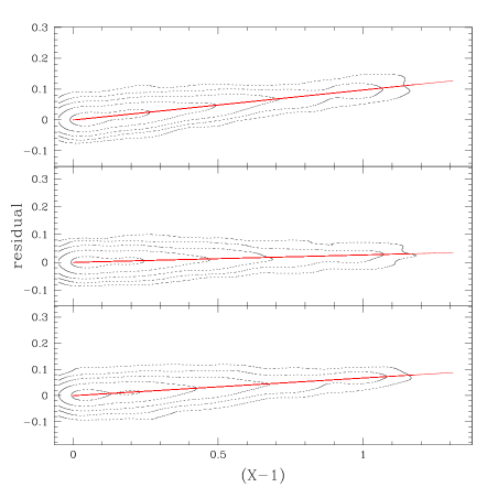
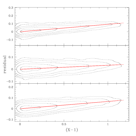
Figure 5: Density plots of the residuals (without the extinction term) as a function of the airmass. Left: Northern solution; Right: Southern solution. Vertical axis is in units of magnitudes. Contour levels are logarithmic, corresponding to point density of 0.3, 1, 3, 10 and 30 mag^-1 airmass^-1. The slopes of the straight lines are the derived mean atmospheric extinction coefficients listed in Table 2.

Given the time baseline of 2MASS and the homogeneity and accuracy of 2MASS photometric data, we have a great opportunity for studying atmospheric extinction in the near-infrared over the period of more than a year. Figure 6 shows the seasonal variations in atmospheric extinction. The monthly averages were derived by, first, calculating the residuals without the extinction term for each month separately, and then, by fitting a straight line to the distribution of residuals as a function of the airmass.

Figure 6: Seasonal variations in the atmospheric extinction (in mag/airmass) in the North (left panel) and in the South (right panel). Monthly average coefficients in $J$, $H$, and $K_{s}$ are plotted with triangles, squares, and circles, respectively. The errors are indicated. Horizontal dashed lines show global averages in three bands derived from the respective GPC solutions. No August data for the Northern solution were available.

While some scatter is present in Figure 6, the overall behavior of monthly extinction averages is in agreement with expectations. The water vapor content in the atmosphere peaks during Northern spring and summer, which leads to higher atmospheric extinction in the North during that season. The amplitude of the seasonal changes is about $0.02$ magnitudes/airmass.

3.3 Global Consistency

The global consistency of the solution can be assessed from the analysis of residuals as a function of spatial coordinate (spatial uniformity) or time (temporal uniformity). In this section, we present the results of two such analyses. First, we examine the uniformity of the standards between the hemispheres, from looking at residuals $\Delta m=m_{North}-m_{South}$ for common calibration fields. Then, we test spatial and temporal uniformity by comparing the calibrated magnitudes of primary standards (derived from GPC) with literature photometry.

3.3.1 North vs. South Uniformity

The linearity of the GPC solution is demonstrated in Figure 7, which shows the difference between catalog and GPC magnitudes for primary standards as a function of the catalog magnitude.

Figure 7: The difference between catalog and GPC magnitudes as a function of catalog magnitude for primary standards. Symbols represent $J$, $H$, and $K_{s}$ magnitudes (crosses, triangles and squares, respectively). Most data points differ from zero by less than 0.02 mag. Note the absence of any trends over the entire magnitude range.

The figure shows that the absolute value of the difference for most primaries is less than 0.02 magnitude, i.e. consistent with zero. The absence of any trends in these data demonstrates the linearity of the GPC solution. Note that the results of such comparison are limited by the accuracy of input catalog since the errors in the fiducial magnitudes of primary standards are propagated unchanged. In fact, the good agreement demonstrates the high accuracy of the input catalog.

The comparison of the photometry between the hemispheres is carried out in equatorial fields (see Table 1). Data from each hemisphere were calibrated separately by unconstrained GPC. The solutions (nightly photometric constants $a$ and $b$, and extinction parameter $A$) were applied to the 100 brightest stars in each calibration field. Figure 8 shows the difference between calibrated magnitudes of common stars as the function of coordinate. Except for a few outliers, the largest excursions for individual secondary standards (crosses) are bounded by $\Delta m<0.04$, while the largest excursions for the primary standards (squares) are less than $0.02$ mag. The mean differences for the photometry of common standards (squares in Figure 8) are $0.002\pm 0.007$ ($J$), $-0.002\pm 0.007$ ($H$), and $-0.001\pm 0.008$ ($K_{s}$). The plot of North-South photometric offset vs. declination displays a slight trend of unknown origin. The slopes of the corresponding regression lines in $J$, $H$, and $K_{s}$ are $(-4.9\pm 0.9)\times 10^{-4}$ mag/deg, $(-7.5\pm 0.9)\times 10^{-4}$ mag/deg, and $(-3.9\pm 0.6)\times 10^{-4}$ mag/deg, respectively. The same regression analysis using primary standards only gives slopes consistent with zero at the $2\sigma$ level: the corresponding slopes are $(-4.9\pm 2.8)\times 10^{-4}$ in $J$, $(-5.2\pm 2.8)\times 10^{-4}$ in $H$, and $(-0.4\pm 3.5)\times 10^{-4}$ in $K_{s}$.

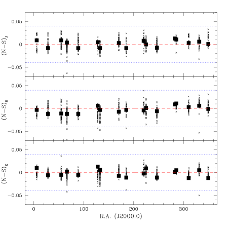
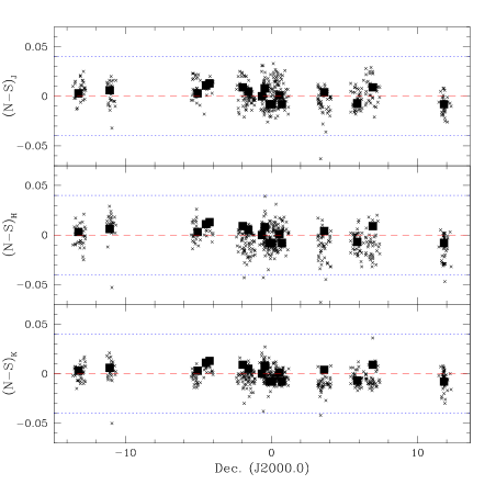
Figure 8: ‘North-South’ difference between calibrated magnitudes of stars in common fields as a function of right ascension (left panel) and declination (right panel). Crosses represent field stars, squares represent primary standards. Clusters of points are calibration fields. Due to elongated shape of calibration fields in latitude, the clusters are more dispersed in the right panel. Dotted horizontal lines are drawn at $\Delta_{m}=\pm 0.04$, dashed line is at zero.

Figure 9 shows the same residuals as in Figure 8, except as a function of magnitude in the North. The slopes of the regression lines in all three bands are consistent with zero.

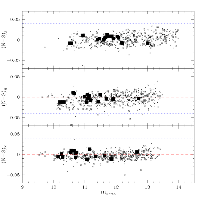
Figure 9: Difference (in magnitudes) between Northern and Southern solutions as a function of Northern magnitude. The notations are the same as in Figure 8.

3.3.2 Temporal Stability

To analyze the temporal stability, we consider the difference between calibrated and fiducial magnitudes of primary standards as a function of time. Specifically, we calculate the difference ‘calibrated-fiducial’ for all primary standards observed on a given night and plot the average difference. Figure 10 shows the corresponding differences in all three bands for Northern and Southern hemispheres.

Figure 10: Difference between calibrated and fiducial magnitude for primary standards as a function of time for Northern (left panel) and Southern (right panel) solutions. Each survey night is represented by a single point which displays the average difference for all standards observed on that night.

The figure, which essentially indicates the long-term stability of the global calibration, shows a very small temporal variation in the photometry of the primary standards. The amplitude of the variations is less than $1\%$.

4 Summary

• We have presented a global photometric calibration procedure and applied it to more than a year of 2MASS calibration data. Exploiting the fact that the observed nightly zeropoint drift is linear, one can simultaneously calibrate the photometry of fiducial standards and any number of tracer stars. The solution is found by using a standard least squares algorithm and is globally optimized, in the sense that it is best solution for all survey fields and nights. The solution does not presume a priori knowledge of the magnitudes for any of the stars, but instead produces the optimal set of relative magnitudes. A constant offset is determined by averaging the differences between the calibrated and catalog magnitudes for the primary standards.

• The photometry of the primary and two tracer stars per field is transferred to the 100 brightest non-variable stars in each field. With a $\sigma$-threshold, we select a low-dispersion sample of 2177 candidate secondary standards to accompany the set of primary 2MASS standards. The selected secondaries fall in the magnitude range $9.0<J<14.5$, $9.0<H<13.9$, $9.0<K_{s}<13.7$.

• Using the global solution, we derive the atmospheric extinction. The global averages are $A_{J}/A_{H}/A_{K_{s}}=0.096/0.026/0.066$ (North), and $A_{J}/A_{H}/A_{K_{s}}=0.092/0.031/0.065$ (South). The averages are consistent with previous work at the $2\sigma$ level.

• Seasonal variations in the atmospheric extinction are analyzed. The amplitude of the variations is approximately $0.02$ mag/airmass and is consistent with the behavior expected from variations of the water vapor content in the atmosphere.

Appendix A Least Squares

The set of equations (2) represents a linear least squares (LLS) problem. The general LLS problem is well-documented in the literature (e.g., Lawson & Hanson 1973, Greenbaum 1986) and has many professional codes available for its solution. Written in the matrix form, the mathematical model for the GPC is

$$\Phi{\bf x}={\bf b},$$ (A1)

where $\Phi$ is the design matrix, ${\bf x}$ is the parameter vector and ${\bf b}$ is the vector of observed (instrumental) magnitudes. The parameter vector ${\bf x}$ consists of the magnitudes of the fiducial standards in each field, followed by the magnitudes of the tracer stars for each field, followed by the photometric nightly constants $a$, $b$ for each night and the atmospheric extinction coefficient $A$:

$${\bf x}^{T}=\left(m^{std}_{1},\ldots,m^{std}_{k},m^{0}_{11},\ldots,m^{0}_{\mu 1},\ldots,m^{0}_{1k},\ldots,m^{0}_{\mu k},a_{1},\ldots,a_{n},b_{1},\ldots,b_{n},A\right),$$ (A2)

where $k$ denotes the total number of calibration fields and $n$ denotes the total number of observation nights. The number of tracers in the field is $\mu$ (the same number of tracers in each field is used). The design matrix $\Phi$ has the following structure:

$$\Phi=\left(\begin{array}[]{ccccc}\overbrace{\mathstrut 1,0,\ldots,0}^{k\ \mathrm{standards}}&\overbrace{\mathstrut 0,0,\ldots,0}^{\mu\times k\ \mathrm{tracers}}&\overbrace{\mathstrut 1,0,\ldots,0}^{n\ \mathrm{nights}}&\overbrace{\mathstrut\Delta t_{jn},0,\ldots,0}^{n\ \mathrm{nights}}&X_{jn}-1\\ {0,1,\ldots,0}&{0,0,\ldots,0}&{1,0,\ldots,0}&{\Delta t_{jn},0,\ldots,0}&X_{jn}-1\\ {0,1,\ldots,0}&{0,0,\ldots,0}&{0,1,\ldots,0}&{0,\Delta t_{jn},\ldots,0}&X_{jn}-1\\ {\ldots}&{\ldots}&{\ldots}&{\ldots}&{\ldots}\\ {0,0,\ldots,0}&{1,0,\ldots,0}&{1,0,\ldots,0}&{\Delta t_{jn},0,\ldots,0}&X_{jn}-1\\ {\ldots}&{\ldots}&{\ldots}&{\ldots}&{\ldots}.\end{array}\right)$$

The tracer stars are grouped by the fields, i.e. after the fiducial standards, there are $n$ tracers from the first field, then there are $n$ tracers from the second field, and so on. There is a single unity in the first $k(\mu+1)$ columns of each row of the design matrix, representing the observation of either the fiducial standard or a tracer star. The subscript $j$ denotes the time offset from the midnight on the night $n$. The dimensions of the matrix are $N\times M$, where $N$ is the total number of observations of all fiducial standards and tracers, and $M=k(\mu+1)+2n+1$ is the number of free parameters.

A.1 Constrained Scheme

The least squares solution of the equations (2) is globally optimal (i.e., it minimizes rms), but, generally speaking, has an arbitrary offset from the true magnitude:

$$\left(m^{\lambda,0}_{ik}\right)_{true}=\left(m^{\lambda,0}_{ik}\right)_{sol}+K_{ik}.$$ (A3)

To produce the optimal solution without the arbitrary additive constant $K_{ik}$ one has to set the magnitudes of the fiducial standards as fixed points of the GPC. This results into GPC with constraints, where the constraint equations are:

$$m^{std}_{ijkn}=m^{std,0}_{ik}$$ (A4)

(the superscript $std$ denotes the fiducial standards in the fields). In the matrix form, the calibration problem with constraints is written as

$$\Phi{\bf x}={\bf b},$$

$$C{\bf x}={\bf d}.$$

For this particular problem, the constraint equations (A4) result in the identity constraint matrix $C$, and the LLS problem with constraints is straightforward to solve using, e.g., orthogonal basis for the null space of the constraint matrix (Lawson & Hanson 1973, Ch. 20). The GPC with fixed points derives the globally optimal solution which is the closest to the listed magnitudes of the fiducial standards.

Appendix B Secondary Standards

Below, we present a sample table of 2MASS secondary standards, which includes the primary and some of the secondaries for the field 90021. The primary standard is the first star listed in each field in Table 3. Columns in the table are $\alpha_{J2000}$, $\delta_{J2000}$ coordinates of the stars, the globally calibrated $JHK_{s}$ magnitudes with the corresponding uncertainties, and the number of observations (i.e. individual scans) in each band. The positions of the secondaries are accurate with respect to the ICRS to $<0.5^{\prime\prime}$ rms. Finding charts for the secondaries can be obtained by using 2MASS Visualizer tool at http://irsatest.ipac.caltech.edu:8001/applications/2MASS/ReleaseVis/. The full table of candidate secondary standards in all calibration fields is available from FTP archives at ftp://nova.astro.umass.edu/pub/nikolaev/, or at ftp://anon-ftp.ipac.caltech.edu/pub/2mass/globalcal/.

Table 3: 2MASS Secondary Standards (sample). Columns list J2000.0 coordinates of the stars. $JHK_{s}$ magnitudes and their rms errors and the number of observations in each band.

$\alpha$ (J2000)	$\delta$ (J2000)	J	$\sigma_{J}$	H	$\sigma_{H}$	$K_{s}$	$\sigma_{K_{s}}$	$N_{J}$	$N_{H}$	$N_{K_{s}}$
Field: 90021
6.10250	$-1.97230$	11.862	0.016	11.081	0.016	10.559	0.018	793	823	817
6.03858	$-2.26631$	13.862	0.029	13.258	0.032	13.148	0.044	450	464	463
6.04265	$-2.28167$	11.922	0.026	11.556	0.025	11.485	0.026	740	767	762
6.04303	$-2.02408$	11.893	0.019	11.243	0.019	11.089	0.019	748	775	770
6.04514	$-1.71895$	11.367	0.019	10.881	0.019	10.798	0.019	768	798	792
6.05158	$-2.04839$	13.702	0.022	13.211	0.023	13.136	0.030	781	811	805
6.05168	$-1.86255$	13.552	0.022	13.241	0.024	13.189	0.033	781	811	805
6.05223	$-2.01792$	13.260	0.019	12.845	0.021	12.766	0.025	781	811	805
6.05384	$-2.27687$	13.055	0.025	12.585	0.029	12.498	0.032	785	815	809
6.05452	$-1.83307$	13.208	0.021	12.893	0.024	12.823	0.028	787	817	811
6.06506	$-2.16824$	13.885	0.025	13.405	0.027	13.326	0.033	793	823	817
6.07232	$-1.62850$	13.781	0.022	13.138	0.025	12.940	0.027	793	823	817
6.07362	$-2.16577$	13.477	0.023	12.864	0.022	12.628	0.025	793	823	817
6.07832	$-1.69025$	14.195	0.026	13.497	0.029	13.328	0.032	793	823	817
6.08807	$-2.31853$	14.019	0.031	13.366	0.035	13.180	0.041	793	823	817
6.08952	$-1.87956$	13.329	0.020	12.750	0.021	12.510	0.024	793	823	817
6.09105	$-2.34330$	12.415	0.023	11.870	0.025	11.772	0.026	793	823	817
6.09865	$-1.55405$	12.306	0.018	11.971	0.022	11.915	0.022	793	823	817
6.09878	$-1.98499$	12.144	0.016	11.545	0.017	11.431	0.018	793	823	817
6.10086	$-2.39661$	12.621	0.020	11.974	0.020	11.847	0.021	793	823	817

References

- (1) Casali, M. & Hawarden, T. 1992, JCMT-UKIRT Newsl., No. 4, 33
- (2) Greenbaum, A. 1986, Iterative Methods for Solving Linear Systems (Philadelphia: SIAM)
- (3) Hall, D. S. & Genet, R. M. 1982, Photoelectric Photometry of Variable Stars (Fairborn, OH: IAPPP)
- (4) Lawson, C. L. & Hanson, R. J. 1995, Solving Least Squares Problems (Philadelphia: SIAM)
- (5) Manduca, A. & Bell, R. A. 1979, PASP, 91, 848
- (6) Mountain, C. M., Leggett, S. K., Selby, M. J., and Zadrozny, A. 1985, A&A, 150, 281
- (7) Persson, S. E., Murphy, D. C., Krzeminski, W., Roth, M., Rieke, M. J. 1998, AJ, 116, 2475