Gravitational Time Delay Effects on CMB Anisotropies

Abstract

We study the effect of gravitational time delay on the power spectra and bispectra of the cosmic microwave background (CMB) temperature and polarization anisotropies. The time delay effect modulates the spatial surface at recombination on which temperature anisotropies are observed, typically by $\sim$ 1 Mpc. While this is a relatively large shift, its observable effects in the temperature and polarization fields are suppressed by geometric considerations. The leading order effect is from its correlation with the closely related gravitational lensing effect. The change to the temperature-polarization cross power spectrum is of order $0.1\%$ and is hence comparable to the cosmic variance for the power in the multipoles around $\ell\sim 1000$. While unlikely to be extracted from the data in its own right, its omission in modeling would produce a systematic error comparable to this limiting statistical error and, in principle, is relevant for future high precision experiments. Contributions to the bispectra result mainly from correlations with the Sachs-Wolfe effect and may safely be neglected in a low density universe.

]

I Introduction

In order that the full potential of anisotropies in the cosmic microwave background (CMB) temperature and polarization fields be realized, effects that have been previously dismissed as negligible in their own right must now be reconsidered as potential sources of systematic error. Projections as to the ability of CMB experiments to measure fundamental cosmological quantities [2] precisely and reveal information about the structure formation process from secondary effects [3] rely on the fact that statistical errors from the sampling of a finite sky rapidly decrease toward smaller angular scales. Statistical errors in the power spectra decline from $\sim 1\%$ at degree scales to $\sim 0.1\%$ at the several arcminute scale. To achieve this precision in practice, all physical, astrophysical and instrumental effects at this level must be included in the analysis to avoid generating systematic errors that are comparable to the statistical errors.

A host of physical effects contribute to the anisotropies at second order in perturbation theory [4, 5, 6, 7]. Since primary anisotropies are formed at recombination when the cosmological density perturbations are at the $10^{-5}$ level, most second order effects are entirely negligible. There are two general ways in which higher order effects can be important. Firstly, the primordial perturbations responsible for the primary anisotropies grow into non-linear structures today by gravitational instability. Effects that take advantage of this fact mainly involve scattering of CMB photons at low redshifts in large-scale structure and non-linear objects [8, 9, 10, 11]. Secondly, since recombination, CMB photons propagate across essentially the whole horizon volume. Intrinsically small effects can accumulate along the path. Indeed it is well known that the gravitational lensing of CMB photons has a substantial effect on the power spectrum of the anisotropies [12, 13].

In addition to the lensing effect, gravitational potentials of large-scale structure contributes a time-delay [14] that accumulates along the path – an effect familiar from studies of the light-curves of lensed quasars (e.g. [15]). In the case of the CMB, the time-delay warps the spatial surface at recombination from which the primary anisotropies arise [6]. Because the lensing depends on the angular gradient of the projected potentials whereas the delay depends on the projected potential itself, the fractional delay is generically smaller than lensing and has not been explicitly calculated in the literature. We shall see however that because of the angular smoothness (or coherence) of the lensing, the reduction in amplitude is not in and of itself large. Furthermore, gravitational time delays are strongly correlated with lensing, leading to additional effects in the power spectrum. Indeed, the typical perturbation in comoving units is on the order of $1$ Mpc. The effect of gravitational time-delay on the spectra of temperature and polarization anisotropies therefore merits further study.

In §II we present the formalism required to understand these gravitational effects on the temperature and polarization fields. We proceed in §III and IV to evaluate the delay and lensing-delay correlation effects on the power spectra of temperature and polarization anisotropies respectively. In §V, we consider their effects on the bispectra (three point correlations). We conclude in §VI with a discussion of our results.

To illustrate our calculations, we assume a cold dark matter model (CDM) with a cosmological constant ($\Lambda$) with parameters $\Omega_{c}=0.30$ for the CDM density, $\Omega_{b}=0.05$ for the baryon density, $\Omega_{\Lambda}=0.65$ for the vacuum density, $h=0.65$ for the dimensionless Hubble constant and a scale invariant spectrum of primordial fluctuations, normalized to COBE [16].

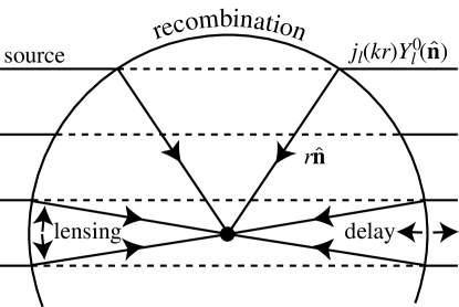
FIG. 1.: Gravitational Lensing vs. Time Delay. Lensing introduces an angular perturbation in the mapping of a plane-wave source field at recombination onto anisotropies today. Time delay introduces a radial modulation. When the wavevector is perpendicular to the line-of-sight, features in the angular spectrum – such as the acoustic peaks – are created, geometrically distinguishing the otherwise similar lensing and delay effects.

II Formalism

As the CMB photons propagate to the observer from the recombination epoch ($z\sim 10^{3}$) through large-scale structure in the universe, they suffer the effects of gravitational lensing and time delay. These effects are both formally second order in perturbation theory because they would leave a homogeneous and isotropic CMB unperturbed (c.f. [17]). There are a host of other second order effects [4, 5, 6]. To the extent that they are uncorrelated with each other, they may be viewed as independent effects. The lensing and time delay effects are strongly correlated because both arise from the gravitational potentials of large scale structure and must be considered together. We therefore begin with a review of lensing effects.

A Lensing

FIG. 2.: Power spectra for the lensing deflection angles (${\phi}{\phi}$), time-delay (${d}{d}$) and deflection-delay cross correlation (${\phi}{d}$). The underlying lensing potential spectrum $C_{\ell}^{{\phi}{\phi}}$ and cross spectrum $C_{\ell}^{{\phi}{d}}$ are weighted by $\ell(\ell+1)$ and $[\ell(\ell+1)]^{1/2}$ respectively to reflect the angular gradients in the deflection angles.

Lensing involves a deflection that remaps the temperature and polarization fields according to the angular gradient of the lensing-weighted projected potential $\hat{\bf n}\rightarrow\hat{\bf n}+\nabla\phi(\hat{\bf n})$ (see Fig. 1)

$$\phi(\hat{\bf n})=-2\int d\eta g_{\phi}(\eta)\Phi(r\hat{\bf n},\eta)\,,$$ (1)

where

$$g_{\phi}(\eta)={1\over r}\int_{0}^{\eta}d\eta^{\prime}\,\dot{\tau}e^{-\tau}{r^{\prime}-r\over r^{\prime}}\,.$$ (2)

Here overdots represent derivatives with respect to conformal time $\eta=\int dt/a$ and $\Phi({\bf x},\eta)$ is the gravitational potential. In an open universe, the conformal distance traveled by a photon $r(\eta)=\eta_{0}-\eta$ should be replaced by angular diameter distances. We take comoving units where $c=1$ throughout. The projected potential itself is a field on the sky and may be decomposed into multipole moments

$${\phi}(\hat{\bf n})=\sum_{\ell m}{\phi}_{\ell m}Y_{\ell}^{m}(\hat{\bf n})\,,$$ (3)

and described by its power spectrum

$$\left<{\phi}_{\ell m}^{*}{\phi}_{\ell^{\prime}m^{\prime}}\right>=\delta_{\ell,\ell^{\prime}}\delta_{m,m^{\prime}}C_{\ell}^{{\phi}{\phi}}\,.$$ (4)

This power spectrum is shown in Fig. 2.

A useful measure of the amplitude of the lensing effects is the rms deflection angle $\theta_{{\rm rms}}^{2}$ as defined by

$$\theta_{{\rm rms}}^{2}=\sum_{\ell=1}^{\infty}{2\ell+1\over 4\pi}\ell(\ell+1)C_{\ell}^{{\phi}{\phi}}\,.$$ (5)

The factor $\ell(\ell+1)$ reflects the angular gradient in the definition of the deflection. Note that the $\ell=0$ monopole does not contribute since its angular gradient vanishes. In the fiducial $\Lambda$CDM model $\theta_{{\rm rms}}=7.5\times 10^{-4}$ or $2.6^{\prime}$. Note that this is in sharp contrast with the angular coherence of the deflection angle. The variance $\theta_{{\rm rms}}^{2}$ reaches half its total value by $\ell_{1/2}=30$ in the fiducial model or an angle of $\theta_{1/2}\equiv 2\pi/\ell_{1/2}\approx 0.02$ ($1^{\circ}$). The smaller scale potential fluctuations tend to produce deflections that cancel out along the line of sight.

B Time Delay

Now consider the time-delay effect. Photons follow null geodesics in the perturbed metric so that in the fixed time interval since last scattering, the distance traveled by the photons is perturbed as $r\rightarrow r[1+d(\hat{\bf n})]$ (see Fig. 1) where

$$d(\hat{\bf n})=-{2\over\eta_{0}}\int d\eta e^{-\tau}\Phi(r\hat{\bf n},\eta)\,.$$ (6)

This is referred to in the literature as the potential or Shapiro time delay. The geometric time delay is of order the deflection angle squared and is hence substantially smaller for time-delays across angular scales much larger than $\theta_{{\rm rms}}$.

The delay field may also be expanded in spherical harmonics

$${d}(\hat{\bf n}) = \sum_{\ell m}{d}_{\ell m}Y_{\ell}^{m}(\hat{\bf n})\,,$$ (7)

and characterized by a power spectrum

$$\left<{d}_{\ell m}^{*}{d}_{\ell^{\prime}m^{\prime}}\right> = \delta_{\ell,\ell^{\prime}}\delta_{m,m^{\prime}}C_{\ell}^{{d}{d}}\,.$$ (8)

Although both the lensing and time-delay effects are based on the gravitational potential projected along the line of sight, there is an important difference between the two. Lensing depends on the angular gradient of the potential and hence its observable consequences are weighted by $\ell(\ell+1)$. This has the effect of increasing the magnitude of the effects and weighting it to higher multipoles.

We can see these effects in the rms delay [19]

$$d_{{\rm rms}}^{2}=\sum_{\ell=1}^{\infty}{2\ell+1\over 4\pi}C_{\ell}^{{d}{d}}\,.$$ (9)

For the power spectrum of the fiducial $\Lambda$CDM model (see Fig. 2) $d_{{\rm rms}}=5.4\times 10^{-5}$ or $\sim 0.5h^{-1}$ Mpc. Although this is a relatively large shift, we shall see that its observable consequences are reduced due to the large coherence scale of the delay, $\ell_{1/2}=2$.

Given these considerations as to the magnitude and coherence scale of the effects, delay effects can be enhanced through their cross-correlation with lensing

$$\left<{\phi}_{\ell m}^{*}{d}_{\ell^{\prime}m^{\prime}}\right> = \delta_{\ell,\ell^{\prime}}\delta_{m,m^{\prime}}C_{\ell}^{{\phi}{d}}\,.$$ (10)

The two fields tend to be well correlated as can be seen by the rms

$$c_{{\rm rms}}^{2}=\sum_{\ell=1}^{\infty}{2\ell+1\over 4\pi}\sqrt{\ell(\ell+1)}C_{\ell}^{{\phi}{d}}\,,$$ (11)

where $c_{{\rm rms}}=1.2\times 10^{-4}$ and $\ell_{1/2}=5$ in the fiducial $\Lambda$CDM model (see Fig. 2). To evaluate the observable consequences, we now turn to the angular and spatial structure of the temperature and polarization fields.

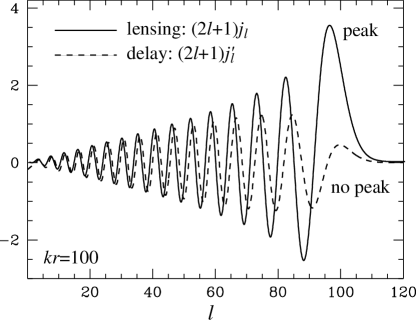
FIG. 3.: Projection functions for the lensing and delay effects. Lensing involves $j_{\ell}(kr)$ whose strong peak in $\ell$ can retain source features; the $j_{\ell}^{\prime}(kr)$ of the time-delay cannot. The product of these functions reflects the cross correlation and is suppressed due to the phase difference.

C Temperature Field

The CMB temperature field on the sky may be written implicitly as the projection of sources $S$ which contribute in the optically thin regime and are so weighted by $e^{-\tau}$ where $\tau$ is the optical depth (see Fig. 1). In general, these sources have intrinsic angular structure of their own and are characterized by the spherical harmonic moments of their Fourier amplitude $S_{\ell_{\rm i}}^{m_{\rm i}}(k)$. Explicit forms for the sources are given in [18].

The contribution from a given wavenumber $k$ to the temperature field on the sky today may be formally expressed as

$$\Theta(\hat{\bf n};{\bf k})=\int_{0}^{\eta_{0}}d\eta e^{-\tau}\sum_{\ell_{\rm i}m_{\rm i}}S_{\ell_{\rm i}}^{m_{\rm i}}(\eta;k)G_{\ell_{\rm i}}^{m_{\rm i}}(r\hat{\bf n};{\bf k})\,,$$ (12)

where $r\equiv\eta_{0}-\eta$,

$$G_{\ell}^{m}({\bf x};{\bf k})=(-i)^{\ell}\sqrt{4\pi\over 2\ell+1}Y_{\ell}^{m}(\hat{\bf n})\exp(i{\bf k}\cdot{\bf x})\,.$$ (13)

In an open universe, the plane waves must be replaced with eigenfunctions of the Laplacian in a curved space. Note that we will often omit the $k$-index where no confusion will arise.

The angular structure of these relations can be simplified by considering a specific frame where ${\bf z}\parallel{\bf k}$ and

$$\exp(i{\bf k}\cdot{\bf x})=\sum(-i)^{\ell}\sqrt{4\pi(2\ell+1)}j_{\ell}(kr)Y_{\ell}^{0}(\hat{\bf n})\,.$$ (14)

Provided that the angular basis does not change in transit, one can then sum up the orbital angular momentum from the plane wave with the intrinsic angular momentum of the source. This assumption is the angular equivalent of the “Born approximation” where the lensing is evaluated on unperturbed trajectories; we shall see in the next section that it is a good approximation for the lensing and time-delay effects on sources with low order intrinsic angular structure.

In this special basis, the product of the intrinsic ($Y_{\ell_{\rm i}}^{m_{\rm i}}$) and plane wave ($Y_{\ell}^{0}$) angular momentum may be reexpressed through the addition of angular momentum. The temperature field then becomes [18]

$$\Theta(\hat{\bf n};{\bf k}) \equiv \sum_{\ell m}\Theta_{\ell m}(k)Y_{\ell}^{m}(\hat{\bf n})$$ (15)

$$= \sum_{\ell m_{\rm i}}I_{m_{\rm i}}[j_{\ell}]Y_{\ell}^{m_{\rm i}}(\hat{\bf n})\,.$$ (16)

Here, the operator

$$I_{m_{\rm i}}[j_{\ell}] \equiv \int_{0}^{\eta_{0}}d\eta e^{-\tau}\sqrt{4\pi(2\ell+1)}$$ (18)

$$\quad\times\sum_{\ell_{\rm i}}S_{\ell_{\rm i}}^{m_{\rm i}}(\eta;k)j_{\ell}^{\ell_{\rm i}m_{\rm i}}(kr)\,,$$

and $j_{\ell}^{\ell_{\rm i}m_{\rm i}}$ are linear combinations of $j_{\ell}$ with weights given by the Clebsch-Gordon coefficients of the coupling. The fundamental functions are $j_{\ell}^{00}=j_{\ell}$ (for isotropic perturbations, e.g. gravitational potentials) and

$$j_{\ell}^{22} = \sqrt{{3\over 8}{(\ell+2)!\over(\ell-2)!}}{1\over 2\ell+1}\left[{j_{\ell-2}+j_{\ell}\over(2\ell-1)}+{j_{\ell}+j_{\ell+2}\over(2\ell+3)}\right]\,,$$ (19)

(for transverse quadrupole sources, e.g. gravitational waves). Note $j_{\ell}^{22}\propto j_{\ell}(x)/x^{2}$; we have written it out here to emphasize linearity. Others are given in [18], but can be written in terms of these fundamental functions through integration by parts [23].

Since the basis for the expansion is linked to the direction of ${\bf k}$, integrating over modes to obtain the final power spectrum in principle requires a series of rotations into a fixed basis. In practice, the statistical homogeneity of the source and isotropy of the angular distribution requires that the $k$-modes add in quadrature and the angular power spectrum is independent of $m$ so that we may replace individual multipoles with an average over $m$

$$C_{\ell}^{\Theta\Theta} = \int{dk\over k}{k^{3}\over 2\pi^{2}}{1\over 2\ell+1}\sum_{m}\left<\Theta_{\ell m}^{*}(k)\Theta_{\ell m}(k)\right>\,.$$ (20)

For the primary anisotropies, the power spectrum is simply $C_{\ell}^{\Theta\Theta}=T_{\ell}^{00}$, where

$$T_{\ell}^{ab} = \int{dk\over k}{k^{3}\over 2\pi^{2}}{(k\eta_{0})^{a+b}\over 2\ell+1}\sum_{m_{\rm i}}I_{m_{\rm i}}^{*}[j_{\ell}^{(a)}]I_{m_{\rm i}}[j_{\ell}^{(b)}]\,.$$ (21)

Here we have used the short hand convention that $j_{\ell}^{(0)}\equiv j_{\ell}$, $j_{\ell}^{(1)}\equiv j_{\ell}^{\prime}$ and $j_{\ell}^{(2)}\equiv j_{\ell}^{\prime\prime}$ with primes denoting derivatives with respect to the argument.

FIG. 4.: Power spectra for the angular ($\ell(\ell+1)T_{\ell}^{00}$), radial ($T_{\ell}^{11}$) and angular-radial cross gradients $(\sqrt{\ell(\ell+1)}T_{\ell}^{01})$ of the primary anisotropies. The cross gradient spectrum has been weighted to reflect the $\ell$ contributions from the angular gradient.

For the higher order lensing and delay effects, we expand equation (16) for the temperature field to second order in the relevant quantities

$$\Theta(\hat{\bf n}) = \Theta^{0}(\hat{\bf n})+\Theta^{{\phi}}(\hat{\bf n})+\Theta^{{d}}(\hat{\bf n})$$ (23)

$$\quad+{1\over 2}\Theta^{{\phi}^{2}}(\hat{\bf n})+\Theta^{{\phi}{d}}(\hat{\bf n})+{1\over 2}\Theta^{{d}^{2}}(\hat{\bf n})\,,$$

where $\Theta^{0}(\hat{\bf n})$ is the zeroth order contribution from the primary anisotropies,

$$\Theta^{{\phi}}(\hat{\bf n}) = \sum_{\ell m_{\rm i}}I_{m_{\rm i}}[j_{\ell}]\,\nabla_{i}\phi(\hat{\bf n})\,\nabla^{i}Y_{\ell}^{m_{\rm i}}(\hat{\bf n})\,,$$ (24)

$$\Theta^{{d}}(\hat{\bf n}) = \sum_{\ell m_{\rm i}}I_{m_{\rm i}}[j_{\ell}^{\prime}]\,(k\eta_{0})\,d(\hat{\bf n})\,Y_{\ell}^{m_{\rm i}}(\hat{\bf n})\,,$$ (25)

$$\Theta^{{\phi}^{2}}(\hat{\bf n}) = \sum_{\ell m_{\rm i}}I_{m_{\rm i}}[j_{\ell}]\,\nabla_{i}\phi(\hat{\bf n})\,\nabla_{j}\phi(\hat{\bf n})\,\nabla^{i}\nabla^{j}Y_{\ell}^{m_{\rm i}}(\hat{\bf n})\,,$$ (26)

$$\Theta^{{\phi}{d}}(\hat{\bf n}) = \sum_{\ell m_{\rm i}}I_{m_{\rm i}}[j_{\ell}^{\prime}]\,(k\eta_{0})\,d(\hat{\bf n})\,\nabla_{i}\phi(\hat{\bf n})\,\nabla^{i}Y_{\ell}^{m_{\rm i}}(\hat{\bf n})\,,$$ (27)

$$\Theta^{{d}^{2}}(\hat{\bf n}) = \sum_{\ell m_{\rm i}}I_{m_{\rm i}}[j_{\ell}^{\prime\prime}]\,(k\eta_{0})^{2}\,d(\hat{\bf n})\,d(\hat{\bf n})\,Y_{\ell}^{m_{\rm i}}(\hat{\bf n})\,.$$ (28)

We shall see that the evaluation of these effects reduces to the computation of the higher order derivative power spectra in equation (21). These power spectra are easily evaluated with minimal modifications to the publically available CMBFAST code: we simply replace $j_{\ell}$ with $j_{\ell}^{\prime}$ and $j_{\ell}^{\prime\prime}$ and leave the evolution and integration over the sources unchanged. To the extent that the underlying sources themselves are smooth, integration by parts on equation (21) shows that $T_{\ell}^{(a\pm 1)(b\mp 1)}\approx-T_{\ell}^{ab}$, e.g. $T_{\ell}^{11}\approx-T_{\ell}^{02}=-T_{\ell}^{20}$. This also implies that terms such as $T_{\ell}^{01}=T_{\ell}^{10}$ are suppressed; mathematically this is due to the lack of correlation between $j_{\ell}$ and $j_{\ell}^{\prime}$ (see Fig. 3). These spectra are compared in Fig. 4.

There is an additional effect from lensing due to the fact that sources are in general anisotropic and gravitational lensing changes the angle at which they are viewed. This formally violates the assumption that the orbital and intrinsic angular momentum of sources can simply be added without additional remapping. The anisotropy in the actual sources, however, are confined to $\ell\leq 2$. To obtain an order unity effect, the deflections must change the viewing angle by order unity in radians. To obtain an order unity effect for lensing, the deflections need change the viewing direction by only a wavelength of the angular perturbation $\ell^{-1}$. Thus at sufficiently high observed $\ell$, deflections always win.

D Polarization Field

The complex Stokes parameter $P_{\pm}=Q\pm iU$ of the polarization on the sky can be expressed implicitly as the projection of the quadrupole moments of the photon temperature and polarization distributions at last scattering

$$P_{\pm}(\hat{\bf n};{\bf k}) = \int_{0}^{\eta_{0}}d\eta e^{-\tau}\sum_{m_{\rm i}}Q^{m_{\rm i}}(\eta;k)\,{}_{\pm 2}G_{2}^{m_{\rm i}}(r\hat{\bf n};{\bf k})\,,$$ (29)

where $Q^{m_{i}}=-\dot{\tau}(\sqrt{6}\Theta_{2m}-6E_{2m})/10$ (see [18], for an explicit definition) and

$${}_{\pm 2}G_{2}^{m}({\bf x};{\bf k})=(-i)^{\ell}\sqrt{4\pi\over 2\ell+1}{}_{\pm 2}Y_{2}^{m}(\hat{\bf n})\exp(i{\bf k}\cdot{\bf x})\,.$$ (30)

Here, ${}_{\pm 2}Y_{\ell}^{m}$ are the spin-2 spherical harmonics [20]. A recoupling of the spin spherical harmonics as in equation (14) yields

$$P_{\pm}(\hat{\bf n};{\bf k}) = \sum_{\ell m}[E_{\ell m}(k)\pm iB_{\ell m}(k)]\,{}_{\pm 2}Y_{\ell}^{m}(\hat{\bf n})$$ (31)

$$= \sum_{\ell m_{\rm i}}P_{m_{\rm i}}[{}_{\pm}\alpha_{\ell}]{}_{\pm 2}Y_{\ell}^{m_{\rm i}}(\hat{\bf n})\,,$$ (32)

where the operator

$$P_{m_{\rm i}}[{}_{\pm}\alpha_{\ell}] \equiv \int_{0}^{\eta_{0}}d\eta e^{-\tau}\sqrt{4\pi(2\ell+1)}$$ (34)

$$\quad\times\sum_{\ell_{\rm i}}Q^{m_{\rm i}}(\eta;k){}_{\pm}\alpha_{\ell}^{m_{\rm i}}(kr)\,.$$

Here, ${}_{\pm}\alpha_{\ell}^{m_{\rm i}}=\epsilon_{\ell}^{m_{\rm i}}\pm i\beta_{\ell}^{m_{\rm i}}$ where the latter are combinations of $j_{\ell}$ given in [18] that define the projection of the source onto the $E$ and $B$ polarization modes. For quadrupole sources related to density $(m_{\rm i}=0)$ fluctuations, $\epsilon_{\ell}^{0}=j_{\ell}^{22}$ (see eqn. [19]) and $\beta_{\ell}^{0}=0$ so that there are no contributions to $B$-parity polarization.

The power spectra for the polarization and temperature-polarization cross correlation are defined as

$$C_{\ell}^{FF^{\prime}} = \int{dk\over k}{k^{3}\over 2\pi^{2}}{1\over 2\ell+1}\sum_{m}\left<F_{\ell m}^{*}(k)F_{\ell m}^{\prime}(k)\right>\,.$$ (35)

where $F$ and $F^{\prime}$ take on the values $\Theta$,$E$ and $B$. For the primary polarization, we define $C_{\ell}^{EE}=E_{\ell}^{00}$, $C_{\ell}^{BB}=B_{\ell}^{00}$, $C_{\ell}^{\Theta E}=X_{\ell}^{00}$, where

$$E_{\ell}^{ab} = \int{dk\over k}{k^{3}\over 2\pi^{2}}{(k\eta_{0})^{a+b}\over 2\ell+1}\sum_{m_{\rm i}}P_{m_{\rm i}}^{*}[\epsilon_{\ell}^{(a)}]P_{m_{\rm i}}[\epsilon_{\ell}^{(b)}]\,,$$ (36)

$$B_{\ell}^{ab} = \int{dk\over k}{k^{3}\over 2\pi^{2}}{(k\eta_{0})^{a+b}\over 2\ell+1}\sum_{m_{\rm i}}P_{m_{\rm i}}^{*}[\beta_{\ell}^{(a)}]P_{m_{\rm i}}[\beta_{\ell}^{(b)}]\,,$$ (37)

$$X_{\ell}^{ab} = \int{dk\over k}{k^{3}\over 2\pi^{2}}{(k\eta_{0})^{a+b}\over 2\ell+1}\sum_{m_{\rm i}}I_{m_{\rm i}}^{*}[j_{\ell}^{(a)}]P_{m_{\rm i}}[\epsilon_{\ell}^{(b)}]\,.$$ (38)

Other combinations vanish due to parity considerations. As in equation (21) the indices $a$ and $b$ refer to derivatives of the underlying Bessel functions. The higher order gravitational effects on the polarization field may be evaluated through a second order expansion of the polarization field

$$P_{\pm}(\hat{\bf n}) = P_{\pm}^{0}(\hat{\bf n})+P_{\pm}^{{\phi}}(\hat{\bf n})+P_{\pm}^{{d}}(\hat{\bf n})$$ (40)

$$\quad+{1\over 2}P_{\pm}^{{\phi}^{2}}(\hat{\bf n})+P_{\pm}^{{\phi}{d}}(\hat{\bf n})+{1\over 2}P_{\pm}^{{d}^{2}}(\hat{\bf n})\,,$$

where $P_{\pm}^{0}(\hat{\bf n})$ is the zeroth order contribution from the primary anisotropies,

$$P_{\pm}^{{\phi}}(\hat{\bf n}) = \sum_{\ell m_{\rm i}}P_{m_{\rm i}}[{}_{\pm}\alpha_{\ell}]\,\nabla_{i}\phi(\hat{\bf n})\,\nabla^{i}{}_{\pm 2}Y_{\ell}^{m_{\rm i}}(\hat{\bf n})\,,$$ (41)

$$P_{\pm}^{{d}}(\hat{\bf n}) = \sum_{\ell m_{\rm i}}P_{m_{\rm i}}[{}_{\pm}\alpha_{\ell}^{\prime}]\,(k\eta_{0})\,d(\hat{\bf n})\,{}_{\pm 2}Y_{\ell}^{m_{\rm i}}(\hat{\bf n})\,,$$ (42)

$$P_{\pm}^{{\phi}^{2}}(\hat{\bf n}) = \sum_{\ell m_{\rm i}}P_{m_{\rm i}}[{}_{\pm}\alpha_{\ell}]\,\nabla_{i}\phi(\hat{\bf n})\,\nabla_{j}\phi(\hat{\bf n})\,\nabla^{i}\nabla^{j}{}_{\pm 2}Y_{\ell}^{m_{\rm i}}(\hat{\bf n})\,,$$ (43)

$$P_{\pm}^{{\phi}{d}}(\hat{\bf n}) = \sum_{\ell m_{\rm i}}P_{m_{\rm i}}[{}_{\pm}\alpha_{\ell}^{\prime}]\,(k\eta_{0})\,d(\hat{\bf n})\,\nabla_{i}\phi(\hat{\bf n})\,\nabla^{i}{}_{\pm 2}Y_{\ell}^{m_{\rm i}}(\hat{\bf n})\,.$$ (44)

$$P_{\pm}^{{d}^{2}}(\hat{\bf n}) = \sum_{\ell m_{\rm i}}P_{m_{\rm i}}[{}_{\pm}\alpha_{\ell}^{\prime\prime}]\,(k\eta_{0})^{2}\,d(\hat{\bf n})\,d(\hat{\bf n})\,{}_{\pm 2}Y_{\ell}^{m_{\rm i}}(\hat{\bf n})\,.$$ (45)

The evaluation of the effects will involve the higher order derivative power spectra of equation (38). Again we modify CMBFAST to calculate these spectra. Just as for the temperature power spectra $E_{\ell}^{(a\pm 1)(b\mp 1)}\approx-E_{\ell}^{ab}$ and similarly for $B$ and $X$. This also implies that terms such as $E_{\ell}^{01}=E_{\ell}^{10}$ are suppressed.

FIG. 5.: Delay, lensing and delay-lensing (cross) perturbations to the CMB temperature power spectrum for the fiducial $\Lambda$CDM model. The cross spectrum dominates the delay spectrum but both produce negligible changes to the primary anisotropies unlike lensing.

III Temperature Power Spectrum

The perturbations to the power spectrum due to the lensing and time-delay effects follow by considering the second order terms in the two-point correlation of the temperature field in equation (23). We can express the contributions schematically as

$$C_{\ell}^{\Theta\Theta}=T_{\ell}^{00}+(T_{\ell}^{{\phi}{\phi}}+T_{\ell}^{{\phi}^{2}})+(T_{\ell}^{{d}{d}}+T_{\ell}^{{d}^{2}})+T_{\ell}^{{\phi}{d}}\,.$$ (46)

We will now define and consider each term in turn.

A Lensing Spectra

The pure lensing contributions can be defined as

$$T_{\ell}^{{\phi}{\phi}} \equiv \int{dk\over k}{k^{3}\over 2\pi^{2}}{1\over 2\ell+1}\sum_{m}\left<\Theta^{{\phi}_{1}*}_{\ell m}\Theta^{{\phi}_{1}}_{\ell m}\right>\,,$$ (47)

$$T_{\ell}^{{\phi}^{2}} \equiv \int{dk\over k}{k^{3}\over 2\pi^{2}}{1\over 2\ell+1}\sum_{m}{1\over 2}\left(\left<\Theta^{{p}*}_{\ell m}\Theta^{{\phi}^{2}}_{\ell m}\right>+{\rm cc.}\right)\,.$$ (48)

Following Ref. [21], we expand the perturbations to the temperature field from equation (24) and the projected potential $\phi$ in spherical harmonics to obtain

$$T_{\ell}^{{\phi}{\phi}} = \sum_{\ell_{1}\ell_{2}}C_{\ell_{1}}^{{\phi}{\phi}}T_{\ell_{2}}^{00}W_{\ell\ell_{1}\ell_{2}}^{2}L_{\ell\ell_{1}\ell_{2}}^{2}\,,$$ (49)

$$T_{\ell}^{{\phi}^{2}} = -{1\over 2}\theta_{\rm rms}^{2}\ell(\ell+1)T_{\ell}^{00}\,,$$ (50)

where

$$W_{\ell\ell_{1}\ell_{2}} = \sqrt{(2\ell_{1}+1)(2\ell_{2}+1)\over 4\pi}\left(\begin{array}[]{ccc}l&l_{1}&l_{2}\\ 0&0&0\end{array}\right)\,,$$ (53)

$$L_{\ell\ell_{1}\ell_{2}} = {1\over 2}[\ell_{1}(\ell_{1}+1)+\ell_{2}(\ell_{2}+1)-\ell(\ell+1)]\,.$$ (54)

The $W_{\ell\ell_{1}\ell_{2}}$ term comes from the integral over the product of three spherical harmonics; the $L_{\ell\ell_{1}\ell_{2}}$ term comes from the conversion of angular gradients into angular Laplacians through integration by parts. On scales where there is power in the primary power spectrum, the two terms in equation (50) nearly cancel. The reason is that the large-angle modulation produced by lensing simply smoothes the features in the power spectrum across $\Delta\ell\sim\ell_{1/2}\approx 30$ [12]. The result of combining the two terms in the fiducial $\Lambda$CDM model is displayed in Fig. 5.

B Delay Spectra

The time-delay modifications to the power spectra can be defined as

$$T_{\ell}^{{d}{d}} \equiv \int{dk\over k}{k^{3}\over 2\pi^{2}}{1\over 2\ell+1}\sum_{m}\left<\Theta^{{d}_{1}*}_{\ell m}\Theta^{{d}_{1}}_{\ell m}\right>\,,$$ (55)

$$T_{\ell}^{{d}^{2}} \equiv \int{dk\over k}{k^{3}\over 2\pi^{2}}{1\over 2\ell+1}\sum_{m}{1\over 2}\left(\left<\Theta^{{p}*}_{\ell m}\Theta^{{d}^{2}}_{\ell m}\right>+{\rm cc}\right)\,,$$ (56)

and their evaluation follows closely that of lensing except for the simplification that no derivatives of spherical harmonics are involved. The result is

$$T_{\ell}^{{d}{d}} = \sum_{\ell_{1}\ell_{2}}C_{\ell_{1}}^{{d}{d}}T_{\ell_{2}}^{11}W_{\ell\ell_{1}\ell_{2}}^{2}\,,$$ (57)

$$T_{\ell}^{{d}^{2}} = d_{{\rm rms}}^{2}T_{\ell}^{02}\,,$$ (58)

where we have used the identity

$$\sum_{m_{1}}Y_{\ell_{1}}^{m_{1}*}Y_{\ell_{1}}^{m_{1}}={2\ell_{1}+1\over 4\pi}\,,$$ (59)

to evaluate

$$\sum_{m_{1}}\int d\hat{\bf n}Y_{\ell}^{m*}Y_{\ell_{1}}^{m_{1}*}Y_{\ell_{1}}^{m_{1}}Y_{\ell_{2}}^{m_{2}}={2\ell_{1}+1\over 4\pi}\delta_{\ell,\ell_{2}}\delta_{m,m_{2}}\,.$$ (60)

The main difference between the lensing and time delay contributions is that the power spectra of the angular gradients of the projected potential $\ell(\ell+1)C_{\ell}^{{\phi}{\phi}}$ and primary temperature anisotropies $\ell(\ell+1)T_{\ell}^{00}$ are replaced by the power spectra of the delay $C_{\ell}^{{d}{d}}$ and that of the radial derivatives of the temperature field $T_{\ell}^{11}\approx-T_{\ell}^{02}$.

As in the case of lensing, the time-delay effect represents a smoothing of the gradient power spectrum $T_{\ell}^{11}$ across a width of $\Delta\ell\sim\ell_{1/2}\approx 2$. The effect is strongly suppressed by the small width of the smoothing and the nearly featureless underlying spectrum $T_{\ell}^{11}$ (see Fig. 4). Contrast this with lensing which has a smoothing width of $\Delta\ell\sim 30$ and an angular gradient power spectrum that shows peaks from the acoustic oscillations. Acoustic features in the power spectrum arise from features in the source power spectrum when the source wavevector is oriented perpendicular to the line of sight. The source then projects with a one-to-one correspondence between angular and physical scale ($\ell=kr$ see Fig. 1). Other alignments contribute to a broad tail to lower multipole moments (see Fig. 3). In the perpendicular orientation, however, a perturbation to the radial distance simply moves the last scattering surface along the crests and troughs of the source leaving no net effect. Mathematically, this effect can be seen in the fact that $j_{\ell}(kr)$ as a function of $\ell$ possesses a strong peak at $\ell=kr$, whereas $j_{\ell}^{\prime}(kr)$ does not (see Fig. 3).

The net effect is therefore much smaller than the naive scaling of the lensing rms (5) and delay rms (9) would imply. It is shown in Fig. 5 for the fiducial model.

C Cross Spectra

The cross correlation between the lensing and delay cause modifications defined by

$$T_{\ell}^{{\phi}{d}} \equiv \int{dk\over k}{k^{3}\over 2\pi^{2}}{1\over 2\ell+1}\sum_{m}\Big{(}\left<\Theta^{{d}_{1}*}_{\ell m}\Theta^{{\phi}_{1}}_{\ell m}\right>$$ (62)

$$+{1\over 2}\left<\Theta^{{p}*}_{\ell m}\Theta^{{\phi}{d}}_{\ell m}\right>+{\rm cc.}\Big{)}\,,$$

The $\Theta^{{\phi}{d}}$ terms are identically zero since

$$\sum_{m}[(\nabla_{i}Y_{\ell}^{m*})Y_{\ell}^{m}+Y_{\ell}^{m*}(\nabla_{i}Y_{\ell}^{m})] = \nabla_{i}\sum_{m}(Y_{\ell}^{m*}Y_{\ell}^{m})$$ (63)

$$= 0\,,$$ (64)

by virtue of the addition theorem of spherical harmonics. The first term reduces to

$$T_{\ell}^{{\phi}{d}} = 2\sum_{\ell_{1}\ell_{2}}C_{\ell_{1}}^{{\phi}{d}}T_{\ell_{2}}^{01}W_{\ell\ell_{1}\ell_{2}}^{2}L_{\ell\ell_{1}\ell_{2}}\,.$$ (65)

Unlike the pure lensing and time delay contributions, there is no second canceling term. However as discussed in §II C, $T_{\ell}^{01}$ is intrinsically small reflecting the lack of correlation between $j_{\ell}$ and $j_{\ell}^{\prime}$ (see Fig. 3). Nonetheless, its net contribution to temperature anisotropy power spectrum is still larger than the pure delay contribution, as a result of the larger amplitude and smaller coherence of the lensing-delay power spectrum $C_{\ell}^{{\phi}{d}}$ (see Fig. 5).

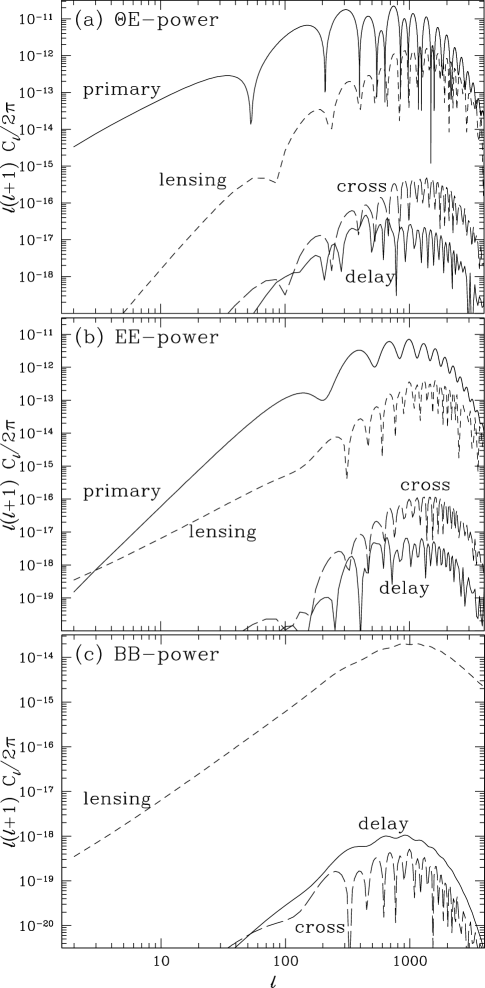
FIG. 6.: Delay, lensing and delay-lensing (cross) contributions to the CMB polarization power spectra for the fiducial $\Lambda$CDM model. The delay-lensing cross contributions to the temperature-polarization power spectrum reaches $10^{-3}$ of the primary and/or lensing power. Delay effects only weakly generate power in the $BB$ spectrum.

IV Polarization Power Spectra

Evaluation of the lensing and delay effects on the polarization and temperature-polarization cross power spectra follows precisely the same steps as that of the temperature power spectrum considered above. We can express the contributions schematically as

$$C_{\ell}^{EE} = E_{\ell}^{00}+(E_{\ell}^{{\phi}{\phi}}+E_{\ell}^{{\phi}^{2}})+(E_{\ell}^{{d}{d}}+E_{\ell}^{{d}^{2}})+E_{\ell}^{{\phi}{d}}\,,$$ (66)

$$C_{\ell}^{BB} = B_{\ell}^{00}+(B_{\ell}^{{\phi}{\phi}}+B_{\ell}^{{\phi}^{2}})+(B_{\ell}^{{d}{d}}+B_{\ell}^{{d}^{2}})+B_{\ell}^{{\phi}{d}}\,,$$ (67)

$$C_{\ell}^{\Theta E} = X_{\ell}^{00}+(X_{\ell}^{{\phi}{\phi}}+X_{\ell}^{{\phi}^{2}})+(X_{\ell}^{{d}{d}}+X_{\ell}^{{d}^{2}})+X_{\ell}^{{\phi}{d}}\,.$$ (68)

We will now consider each term in turn.

A Lensing Spectra

Following [21], the lensing contributions to the polarization power spectra can be evaluated as

$$E_{\ell}^{{\phi}{\phi}} = \sum_{\ell_{1}\ell_{2}}C_{\ell_{1}}^{{\phi}{\phi}}{}_{+}\Sigma_{\ell_{2}}^{00}(\ell+\ell_{1}+\ell_{2})V_{\ell\ell_{1}\ell_{2}}^{2}L_{\ell\ell_{1}\ell_{2}}^{2}\,,$$ (69)

$$E_{\ell}^{{\phi}^{2}} = -{1\over 2}\theta_{\rm rms}^{2}(\ell^{2}+\ell-4)E_{\ell}^{00}\,,$$ (70)

$$B_{\ell}^{{\phi}{\phi}} = \sum_{\ell_{1}\ell_{2}}C_{\ell_{1}}^{{\phi}{\phi}}{}_{-}\Sigma_{\ell_{2}}^{00}(\ell+\ell_{1}+\ell_{2})V_{\ell\ell_{1}\ell_{2}}^{2}L_{\ell\ell_{1}\ell_{2}}\,,$$ (72)

$$B_{\ell}^{{\phi}^{2}} = -{1\over 2}\theta_{\rm rms}^{2}(\ell^{2}+\ell-4)B_{\ell}\,,$$ (73)

$$X_{\ell}^{{\phi}{\phi}} = \sum_{\ell_{1}\ell_{2}}C_{\ell_{1}}^{{\phi}{\phi}}X_{\ell_{2}}^{00}W_{\ell\ell_{1}\ell_{2}}V_{\ell\ell_{1}\ell_{2}}L_{\ell\ell_{1}\ell_{2}}^{2}\,,$$ (75)

$$X_{\ell}^{{\phi}^{2}} = -{1\over 2}\theta_{\rm rms}^{2}(\ell^{2}+\ell-2)X_{\ell}\,,$$ (76)

where

$${}_{\pm}\Sigma_{\ell}^{ab}(L)={[1+(-1)^{L}]\over 2}{E}_{\ell}^{ab}\pm{[1-(-1)^{L}]\over 2}{B}_{\ell}^{ab}\,.$$ (77)

Here

$$V_{\ell\ell_{1}\ell_{2}}=\sqrt{(2\ell_{1}+1)(2\ell_{2}+1)\over 4\pi}\left(\begin{array}[]{ccc}\ell&\ell_{1}&\ell_{2}\\ 2&0&-2\end{array}\right)\,,$$ (78)

comes from the integral over the product of a spherical harmonic with 2 spin-$2$ spherical harmonics. As in the case of the temperature power spectra, the main effect on the $\Theta E$ and $EE$ power spectra is a smoothing by $\Delta\ell\sim\ell_{1/2}$. If there were an intrinsic $BB$ power spectrum, the smoothing would also apply. However, since scalar perturbations do not generate $BB$ modes in the primary polarization ($B_{\ell}^{00}=0$), the generation of $B$-polarization from the lensing modulation of the primary $E$-polarization dominates [13]. The amount of generation is again related to the coherence scale $\ell_{1/2}\approx\ell_{1}$ of the effect as reflected in the difference between even and odd $L$ terms in $V_{\ell\ell_{1}\ell_{2}}$. Considering the triplet as forming a triangle, even terms are associated with the cosine of twice the opening angle between $\ell$ and $\ell_{2}$; odd terms are associated with the sine of that angle ([21], Eqns. (B8) and (B10)). These polarization contributions are shown in Fig. 6 for the fiducial model.

B Delay Spectra

The derivation of the delay power spectra follows the same steps as those involved in the lensing derivation yielding

$$E_{\ell}^{{d}{d}} = \sum_{\ell_{1}\ell_{2}}C_{\ell_{1}}^{{d}{d}}{}_{+}\Sigma_{\ell_{2}}^{11}(\ell+\ell_{1}+\ell_{2})V_{\ell\ell_{1}\ell_{2}}^{2}\,,$$ (79)

$$E_{\ell}^{{d}^{2}} = d_{\rm rms}^{2}E_{\ell}^{02}\,,$$ (80)

$$B_{\ell}^{{d}{d}} = \sum_{\ell_{1}\ell_{2}}C_{\ell_{1}}^{{d}{d}}{}_{-}\Sigma_{\ell_{2}}^{11}(\ell+\ell_{1}+\ell_{2})V_{\ell\ell_{1}\ell_{2}}^{2}\,,$$ (82)

$$B_{\ell}^{{d}^{2}} = d_{\rm rms}^{2}B_{\ell}^{02}\,,$$ (83)

$$X_{\ell}^{{d}{d}} = \sum_{\ell_{1}\ell_{2}}C_{\ell_{1}}^{{d}{d}}X_{\ell_{2}}^{11}W_{\ell\ell_{1}\ell_{2}}V_{\ell\ell_{1}\ell_{2}}\,,$$ (85)

$$X_{\ell}^{{d}^{2}} = d_{\rm rms}^{2}X_{\ell}^{02}\,.$$ (86)

The results of summing these nearly canceling pairs for the fiducial model are shown in Fig. 6. A $BB$-spectrum is generated out of the primary $EE$-spectrum but at an efficiency that is substantially below that of gravitational lensing. The underlying reason again is that the coherence of the effect $\ell_{1/2}\sim 2$.

C Cross Spectra

The cross spectra contributions are defined as

$$E_{\ell}^{\phi{d}} = 2\sum_{\ell_{1}\ell_{2}}C_{\ell_{1}}^{\phi d}{}_{+}\Sigma_{\ell_{2}}^{01}(\ell+\ell_{1}+\ell_{2})V_{\ell\ell_{1}\ell_{2}}^{2}L_{\ell\ell_{1}\ell_{2}}\,,$$ (87)

$$B_{\ell}^{\phi{d}} = 2\sum_{\ell_{1}\ell_{2}}C_{\ell_{1}}^{\phi d}{}_{-}\Sigma_{\ell_{2}}^{01}(\ell+\ell_{1}+\ell_{2})V_{\ell\ell_{1}\ell_{2}}^{2}L_{\ell\ell_{1}\ell_{2}}\,,$$ (88)

$$X_{\ell}^{\phi{d}} = \sum_{\ell_{1}\ell_{2}}C_{\ell_{1}}^{\phi d}(X_{\ell_{2}}^{01}+X_{\ell_{2}}^{10})W_{\ell\ell_{1}\ell_{2}}V_{\ell\ell_{1}\ell_{2}}L_{\ell\ell_{1}\ell_{2}}\,.$$ (89)

Figure 6 shows that the cross spectra dominate over the pure delay spectra for the $\Theta E$ and $EE$ power spectra. In particular, since the lensing effects themselves approach order unity at $\ell\sim 1000$, the lensing-delay cross effects reach $\sim 10^{-3}$ of the primary $C_{\ell}^{\Theta E}$ power spectrum. While still small, the contribution is of order the cosmic variance out to comparable multipoles.

FIG. 7.: Delay-temperature cross correlation. The cross-correlation between the temperature and delay fields, as relevant for the bispectra, are dominated by contributions from the Sachs-Wolfe (SW) effect with partially canceling contributions from the integrated Sachs-Wolfe effect (ISW).

V Delay Bispectrum

Second order effects generally produce non-Gaussianity in the CMB temperature and polarization fields. Effects that provide a negligible change to the power spectrum can in principle produce observable effects due to the expected Gaussianity of the primary anisotropies. Here we consider the three-point correlations induced by time-delay in angular harmonic space, i.e. the bispectrum.

The angle averaged bispectrum is defined as

$$B_{\ell\ell^{\prime}\ell^{\prime\prime}}^{FF^{\prime}F^{\prime\prime}}=\sum_{mm^{\prime}m^{\prime\prime}}\left(\begin{array}[]{ccc}\ell&\ell^{\prime}&\ell^{\prime\prime}\\ m&m^{\prime}&m^{\prime\prime}\end{array}\right)\left<F_{\ell m}F_{\ell^{\prime}m^{\prime}}F_{\ell^{\prime\prime}m^{\prime\prime}}\right>\,,$$ (90)

where the $F$’s can take on the values $\Theta$, $E$, $B$ for the temperature and polarization components respectively. Since the derivation follows closely that of the lensing bispectra terms, we refer the reader to [21] for detailed derivations.

FIG. 8.: Signal-to-noise for detection of bispectra involving gravitational time-delay in an ideal cosmic-variance limited experiment.

A Temperature

The temperature bispectrum produced by time delays follows immediately from the decomposition in equation (24)

$$B_{\ell_{1}\ell_{2}\ell_{3}}^{\Theta\Theta\Theta}=\sqrt{2\ell_{1}+1}W_{\ell_{1}\ell_{2}\ell_{3}}C_{\ell_{2}}^{\Theta d}T_{\ell_{3}}^{01}+{\rm 5perm.}\,,$$ (91)

where the permutations are with respect to the $\ell$-indices and

$$\left<\Theta_{\ell m}^{*}d_{\ell^{\prime}m^{\prime}}\right>=\delta_{\ell\ell^{\prime}}\delta_{mm^{\prime}}C_{\ell}^{\Theta d}\,.$$ (92)

Unlike lensing however, $C_{\ell}^{\Theta d}$ is not solely the result of correlations with secondary anisotropies but includes relatively large contributions from the primary anisotropies themselves. The delay field arises from potential fluctuations of sufficiently large scale that it is correlated with the Sachs-Wolfe effect [22] in the primary anisotropies. To see this, let us approximate the primary anisotropies at large angles as the sum of Sachs-Wolfe (SW) and integrated Sachs-Wolfe (ISW) contributions

$$\Theta(\hat{\bf n})\approx-{1\over 3}\Phi(r_{*}\hat{\bf n},\eta_{*})-\int d\eta^{\prime}\,2\dot{\Phi}(r^{\prime}\hat{\bf n},\eta^{\prime})\,,$$ (93)

where the asterisk denotes evaluation at recombination. This temperature field may be directly correlated with the delay field in equation (6). The resulting power spectrum is shown in Fig. 7. Note that the SW and ISW contributions cancel at the lowest multipoles. Unlike the lensing-ISW correlation [3], the delay effects on the bispectrum do not vanish and indeed increase as $\Omega_{\Lambda}\rightarrow 0$.

To determine whether the contributions are detectable, we evaluate the signal-to-noise ratio for an ideal cosmic variance limited experiment

$$\left({S\over N}\right)_{\Theta\Theta\Theta}^{2}=\sum_{\ell_{1}\ell_{2}\ell_{3}}{(B_{\ell_{1}\ell_{2}\ell_{3}}^{\Theta\Theta\Theta})^{2}\over 6C_{\ell_{1}}^{\Theta\Theta}C_{\ell_{2}}^{\Theta\Theta}C_{\ell_{3}}^{\Theta\Theta}}\,.$$ (94)

We show the cumulative signal-to-noise out to a given maximum $\ell$ in Fig. 8. The time-delay temperature bispectrum is not detectable even for an ideal experiment. This should be compared with the lensing-temperature bispectrum, where the cross-correlation between lensing and effects such as SZ can be detected with upcoming experiments, such as Planck.

B Polarization

Bispectrum terms involving the polarization follow similarly. The non-vanishing contributions are

$$B^{E\Theta\Theta}_{\ell\ell_{1}\ell_{2}} = \sqrt{2\ell_{1}+1}V_{\ell_{1}\ell_{2}\ell_{3}}C_{\ell_{2}}^{\Theta d}X_{\ell_{3}}^{01}$$ (96)

$$\quad+\sqrt{2\ell_{2}+1}W_{\ell_{2}\ell_{1}\ell_{3}}X_{\ell_{1}}^{10}C_{\ell_{3}}^{\Theta d}+(\ell_{2}\leftrightarrow\ell_{3})\,,$$

$$B^{EE\Theta}_{\ell\ell_{1}\ell_{2}} = \sqrt{2\ell_{1}+1}V_{\ell_{1}\ell_{3}\ell_{2}}E_{\ell_{2}}^{10}C_{\ell_{3}}^{\Theta d}+(\ell_{1}\leftrightarrow\ell_{2})\,,$$ (97)

for $\ell_{1}+\ell_{2}+\ell_{3}=$ even and

$$B^{B\Theta\Theta}_{\ell\ell_{1}\ell_{2}} = i\sqrt{2\ell_{1}+1}V_{\ell_{1}\ell_{2}\ell_{3}}C_{\ell_{2}}^{\Theta d}X_{\ell_{3}}^{01}+(\ell_{2}\leftrightarrow\ell_{3})\,,$$ (98)

$$B^{BE\Theta}_{\ell\ell_{1}\ell_{2}} = i\sqrt{2\ell_{1}+1}V_{\ell_{1}\ell_{2}\ell_{3}}E_{\ell_{2}}^{10}C_{\ell_{3}}^{\Theta d}\,,$$ (99)

for $\ell_{1}+\ell_{2}+\ell_{3}=$ odd. The signal-to-noise ratio in an ideal, cosmic variance limited experiment is

$$\left({S\over N}\right)_{E\Theta\Theta}^{2} \approx \sum_{\ell_{1}\ell_{2}\ell_{3}}{(B_{\ell_{1}\ell_{2}\ell_{3}}^{E\Theta\Theta})^{2}\over 6C_{\ell_{1}}^{EE}C_{\ell_{2}}^{\Theta\Theta}C_{\ell_{3}}^{\Theta\Theta}}\,,$$ (100)

$$\left({S\over N}\right)_{EE\Theta}^{2} \approx \sum_{\ell_{1}\ell_{2}\ell_{3}}{(B_{\ell_{1}\ell_{2}\ell_{3}}^{EE\Theta})^{2}\over 6C_{\ell_{1}}^{EE}C_{\ell_{2}}^{EE}C_{\ell_{3}}^{\Theta\Theta}}\,,$$ (101)

$$\left({S\over N}\right)_{B\Theta\Theta}^{2} \approx \sum_{\ell_{1}\ell_{2}\ell_{3}}{(B_{\ell_{1}\ell_{2}\ell_{3}}^{B\Theta\Theta})^{2}\over 2C_{\ell_{1}}^{BB}C_{\ell_{2}}^{\Theta\Theta}C_{\ell_{3}}^{\Theta\Theta}}\,,$$ (102)

$$\left({S\over N}\right)_{BE\Theta}^{2} \approx \sum_{\ell_{1}\ell_{2}\ell_{3}}{(B_{\ell_{1}\ell_{2}\ell_{3}}^{BE\Theta})^{2}\over 2C_{\ell_{1}}^{BB}C_{\ell_{2}}^{EE}C_{\ell_{3}}^{\Theta\Theta}}\,.$$ (103)

In Fig. 8, we show the cumulative signal-to-noise ratio as a function of the maximum $\ell$. The signal-to-noise ratio for the $B\Theta\Theta$ term is larger than the others since we have assumed that $C_{\ell}^{BB}$ vanishes for the primary anisotropies and is only generated by the lensing and delay effects. Nonetheless, the signal-to-noise is substantially less than unity and so the time-delay effects are unlikely to be detectable in the bispectrum or affect the extraction of other effects from the bispectrum.

VI Discussion

Gravitational time delays introduce a radial perturbation in the mapping of the CMB temperature field at recombination onto temperature and polarization anisotropies today. The effect is closely related to gravitational lensing which introduces angular perturbations in the same mapping. Despite the fact that radial perturbations are only one order of magnitude smaller than angular perturbations, and moreover highly correlated with the angular perturbations, their effect on the power spectra and bispectra of the temperature and polarization fields is approximately 3 orders of magnitudes smaller. The underlying reason is that on the angular scales of the acoustic peaks neither effect actually generates new anisotropies; both induce a large scale modulation of the primary field. Angular modulations produce a substantial effect due to angular structure in the acoustic peaks by smoothing the power spectrum on the coherence scale $\Delta\ell\sim 30$. Radial modulations produce much smaller effects due to the lack of radial structure in the perturbations that form the acoustic peaks. They also suffer from the fact that the angular coherence or smoothing scale of the radial modulation is typically one order of magnitude larger $\Delta\ell\sim 2$.

As a result, at $\ell\sim 1000$, the delay and lensing-delay correlation effects are $\lesssim 10^{-4}$ of the temperature, $E$-polarization and lensing-induced $B$-polarization power spectrum generated by lensing. For the temperature-polarization cross correlation, the lensing-delay correlation effect approaches $10^{-3}$ and so is comparable to the cosmic variance on these scales. This enhancement reflects the same efficiency with which lensing modulations affect the temperature-polarization correlation. It is therefore relevant in principle for the Planck satellite or any future experiment that expects to be cosmic variance limited at $\ell\gtrsim 1000$. In practice, there may well be other more limiting sources of systematic errors such as galactic and extragalactic foregrounds.

For the bispectra, the time delay couples mainly with the Sachs-Wolfe effect in the primary anisotropies. For a cosmic variance limited experiment, the signal-to-noise is highest in the $B$-temperature-temperature bispectrum since the $B$-polarization vanishes for primary anisotropies from scalar perturbations. In a realistic experiment, the low level of the signal will make the cosmic variance limit difficult to achieve. In any case, the signal-to-noise ratios in the bispectra never exceed the $10^{-1}$ level for $\ell\sim 1000$ and hence are unlikely to interfere with the extraction of signals in the bispectrum from secondary anisotropies by the next generation of satellites [3].

The potential of cosmic microwave background anisotropies for studying cosmology is considered vast primarily because of the physical processes underlying their formation are thought to be understood to extraordinary precision relative to other astrophysical systems. Though unlikely to affect the next generation of experiments, small effects such as the gravitational time delay considered here must be calculated and included to ensure that this potential is realized.

- [1]
- [2] L. Knox, Phys. Rev. D, 52 4307 (1995); G. Jungman, M. Kamionkowski, A. Kosowsky and D.N. Spergel, Phys. Rev. D, 54 1332 (1995); J.R. Bond, G. Efstathiou and M. Tegmark, MNRAS, 291 L33 (1997); M. Zaldarriaga, D.N. Spergel and U. Seljak, Astrophys. J., 488 1 (1997); D.J. Eisenstein, W. Hu and M. Tegmark, Astrophys. J., 518 2 (1999)
- [3] M. Zaldarriaga and U. Seljak, Phys. Rev. D, 59 123507 (1999); D.M. Goldberg and D.N. Spergel, Phys. Rev. D, 59 103002 (1999); A.R. Cooray, W. Hu and M. Tegmark, Astrophys. J., in press (astro-ph/0002238)
- [4] W. Hu, D. Scott and J. Silk, Phys. Rev. D, 49 648 (1994)
- [5] S. Dodelson and J.M.. Jubas, Astrophys. J., 439 503 (1995)
- [6] T. Pyne and S.M. Carroll, Phys. Rev. D, 53 2920 (1996)
- [7] S. Matarrese, S. Mollerach and M. Bruni, Phys. Rev. D, 58 043504 (1998)
- [8] R.A. Sunyaev and Ya.B. Zel’dovich, Astrophys. Space Scie., 7 1 (1970)
- [9] E. Vishniac, Astrophys. J., 322 597 (1987)
- [10] N. Aghanim, F.X. Desert, J.L. Puget, and R. Gispert, A&A, 311 1 (1996); A. Gruzinov and W. Hu, Astrophys. J., 508 435 (1998); L. Knox R. Scoccimarro and S. Dodelson, Phys. Rev. Lett., 81 2004 (1998)
- [11] W. Hu, Astrophys. J., 529 12 (2000)
- [12] U. Seljak, Astrophys. J., 463 1 (1996)
- [13] M. Zaldarriaga and U. Seljak, Phys. Rev. D, 58 023003 (1998)
- [14] I.I. Shapiro, Phys. Rev. Lett., 13 789 (1964)
- [15] P. Schneider, J. Ehlers and E.E. Falco, Gravitational Lenses (Springer-Verlag, Berlin, 1992)
- [16] E.F. Bunn and M. White, Astrophys. J., 480 6 (1997)
- [17] D.-M. Chen, X.-P. Wu and D.-R. Jiang, Astrophys. J., in press (astro-ph/0007299)
- [18] W. Hu and M. White, Phys. Rev. D, 56 596 (1997)
- [19] We omit in equation (9) which contributes a logarithmically divergent term for scale invariant conditions. The corresponding uniform change to the definition of the length scale would be canceled by second order effects in the fluid description before recombination. Since more subtle cancellations can in principle occur, our calculation is formally an upper bound on the observable consequences of time delays.
- [20] J.N. Goldberg et al., J. Math. Phys, 8 2155 (1967)
- [21] W. Hu, Phys. Rev. D, 62 043007 (2000)
- [22] R.K. Sachs and A.M. Wolfe, Astrophys. J., 147 73 (1967)
- [23] U. Seljak and M. Zaldarriaga, Astrophys. J., 469 437 (1996)