Formation of an Infalling Disklike Envelope around a Protostar

Abstract

We examined the gravitational contraction of isothermal molecular cloud cores with slow rotation by means of two-dimensional numerical simulations. Applying a sink-cell method, we followed the evolution of the cloud cores up to the stages at which most of the matter accretes onto the central region (i.e., a protostar and a rotationally-supported circumstellar disk). We show that both an infalling disklike envelope and a rotationally-supported disk around the central star are natural outcome of the gravitational contraction of a prolate cloud core with slow rotation. The early evolution of the infalling envelopes resembles sheet models recently proposed by Hartmann and coworkers. In the infalling disklike envelope, the radial profiles of the density, radial velocity, and azimuthal velocity can be approximated by $\rho\propto r^{-1.5}$, $v_{r}\propto r^{-0.5}$, and $v_{\varphi}\propto r^{-1}$, respectively. The fate of the infalling envelopes is also discussed.

1 Introduction

Recent high-resolution interferometric observations have suggested that disklike envelopes are common structures around embedded young stars (e.g., Hayashi, Ohashi, & Miyama 1993; Ohashi et al. 1996). In the disklike envelopes, infall motions seem to dominate over the rotation around the young stars, indicating that the disklike envelopes are not rotationally-supported. Thus, embedded young stars are most likely to be undergoing dynamical accretion from their disklike envelopes onto quasi-static protostellar cores and rotationally-supported circumstellar disks. The typical infalling disklike envelope has a size of the order of $10^{3}$ AU, which is an order of magnitude larger in size than a rotationally-supported circumstellar disk observed in the dust emission. The infalling envelopes are expected to play a crucial role in the formation processes of stars as well as their surrounding rotationally-supported disks. It is thus important to understand the formation and evolution of the infalling disklike envelopes.

Several authors have proposed the formation mechanisms of such infalling disks around young stars by means of numerical hydrodynamics. Galli & Shu (1993) examined the gravitational contraction of magnetized spherical cloud cores [see also Boss (1987) and Yorke & Bodenheimer (1999) for the evolution of non-magnetized rotating spherical cloud cores]. They showed that the magnetic field impedes the contraction perpendicular to the field lines and thus the disklike structures develop in the infalling envelopes. In their model, the magnetic field is essential in the formation of the infalling disks. Hartmann et al. (1994) proposed another process for the formation of the infalling disks. They showed that even in the absence of the magnetic field, initially sheetlike cloud cores collapse to form highly disklike envelopes which have similar structures to Galli & Shu (1993)’s disks. Their calculations indicate that the cloud geometry plays an important role in the formation of the infalling envelopes.

Radio observations have shown that most molecular cloud cores are elongated, implying on statistical grounds that most of them are prolate (Myers et al. 1991). Bonnell, Bate, & Price (1996) thus examined the gravitational contraction of non-rotating prolate cloud cores. They found that in a prolate cloud core close to virial equilibrium, the pressure force retards the contraction preferentially along its minor axis. As a result, an extended disklike structure, qualitatively similar to Hartmann et al. (1994)’s sheet model, is formed.

Although these calculations have demonstrated the formation processes of the infalling disks in molecular cloud cores, it is still not clear how the infalling disks form and evolve subsequently and how rotationally-supported circumstellar disks form in the infalling disklike envelopes.

In this paper, we examine the gravitational collapse of prolate cloud cores with slow rotation. We show that both the infalling disklike envelope and rotationally-supported circumstellar disk are natural outcome of the gravitational contraction of a prolate cloud core. In §2, we describe our model and numerical method. Numerical results are given in §3. In §4, we discuss the evolution of the mass infall rate in the disklike envelope. Finally we discuss implications to observations.

2 Models and Numerical Methods

Radio observations have revealed that most molecular clouds have more or less filamentary structures. Recent numerical simulations have also shown that such filaments are ubiquitous features in self-gravitating molecular clouds (e.g., Klessen, Burkert, & Bate 1998). According to a linear stability analysis, the linear perturbation grows fastest in time when its longitudinal wavelength is several times as long as the effective cloud diameter. It is worth noting that in the absence of the strong magnetic fields and fast rotation, the filamentary cloud is unstable to linear perturbations whose wavelengths are more than twice the effective cloud diameter (Matsumoto, Nakamura, & Hanawa 1994). Hence, the fragments tend to become prolate at the epoch of the fragmentation. We investigate the evolution of such prolate fragments formed through the fragmentation of filamentary clouds.

The model cloud is the same as that of Matsumoto, Hanawa, & Nakamura (1997). We consider an isothermal cylindrical cloud in which the density is uniform along the cylinder axis. We assume that the cloud is in hydrostatic equilibrium in the radial direction and that the cloud is rotating around the cylinder axis. The ratio of the centrifugal force to the pressure force, $\beta$, is assumed to be spatially uniform. The radial distributions of the density and velocity are then given by

$$\rho=\rho_{0}\left(1+\frac{r^{2}}{8H^{2}}\right)^{-2}\;,$$ (1)

and

$$\mbox{\boldmath$v$}=(v_{r},v_{\varphi},v_{z})=\left[0,r\Omega_{0}\left(1+\frac{r^{2}}{8H^{2}}\right)^{-1/2},0\right]\;,$$ (2)

respectively, where $H^{2}=(1+\beta)c_{s}^{2}/(4\pi G\rho_{0})$, $\Omega_{0}^{2}=2\pi G\rho_{0}\beta/(1+\beta)$, $c_{s}$ is the isothermal sound speed, $G$ is the gravitational constant, and $\rho_{0}$ is the initial central density. It should be noted that in this model, most of the matter rotates nearly uniformly ($v_{\varphi}\propto r$) and only the outer low-density region with a small mass rotates differentially ($v_{\varphi}={\rm const.}$).

The initial model of our simulation is obtained by adding a velocity perturbation onto the equilibrium model. The velocity perturbation changes sinusoidally with the wavelength of $\lambda_{z}$,

$$\delta v_{z}=v_{0}\sin(2\pi z/\lambda_{z})\;,$$ (3)

where $v_{0}$ is the amplitude of the perturbation and is set to 5% of the sound speed. In the following, we take $\rho_{0}$ and $c_{s}$ as the units of density and velocity, respectively. Then, the initial model is specified by the two parameters of $\beta$ and $\lambda_{z}$. For the typical models, the wavelength $\lambda_{z}$ is taken to be 15.5 $c_{s}/\sqrt{2\pi G\rho_{0}}$, which is almost equal to those of the fastest-growing linear modes for non-rotating or slowly-rotating clouds (Matsumoto et al. 1994). Observationally, most molecular cloud cores are likely to be rotating quite slowly (Goodman et al. 1993). Thus, we adopt the small values of $\beta$ ($=0-0.1$). In Table 1, we summarize the initial conditions of the models calculated in this paper.

We solved numerically the time evolution of the model cloud with the spatially and temporally second-order-accurate hydrodynamical code described by Matsumoto et al. (1997). Since our model keeps mirror symmetry at $z=0$ and $\lambda_{z}/2$ throughout the evolution, we restricted the computational domain in the interval of $0\leq z\leq\lambda_{z}/2$. We set the fixed boundary conditions at $r=0,\ R_{\rm max}$ and $z=0,\ Z_{\rm max}$, where $R_{\rm max}$ and $Z_{\rm max}$ denote the lengths of the computational box in the $r$- and $z$-directions, respectively. For all the models, we take $R_{\rm max}=2Z_{\rm max}=\lambda_{z}$. The effect of the fixed boundary is very small. We have calculated the evolution of the models with larger $R_{\rm max}$ and have confirmed that the numerical results are not changed.

Many numerical simulations have shown that the gravitational collapse of an isothermal cloud accelerates in the central high-density region. Thus, the characteristic length and time scales shorten as the collapse proceeds, this phase being referred to as runaway collapse phase. Therefore, it is difficult to resolve the central high-density region sufficiently at the late stages of the computation even if the cloud evolution is followed with very fine grids. In real evolution, as the collapse progresses, a protostellar core is formed at the center and thereafter the envelope gas begins to accrete onto the central core, this phase being referred to as the accretion phase.

To pursue the evolution of the infalling envelope gas, we adopted a sink-cell method when the central density reaches a reference density $\rho_{\rm sink}$ [see, e.g., Boss & Black (1982) and Tomisaka (1996)]. In this paper, we take $\rho_{\rm sink}=10^{4}\rho_{0}$ and the innermost region of $0\leq r\leq 5\Delta r$ and $0\leq z\leq 5\Delta z$ is assigned to the sink cells, where $\Delta r$ and $\Delta z$ denote the grid spacings in the $r$- and $z$-directions, respectively. The excess density ($\rho-\rho_{\rm sink}$) and the corresponding momentum are removed from the sink cells in every time step. The removed mass is added to a central point mass that affects the matter in the envelope only through gravitation.

As mentioned above, we take $\rho_{0}=1$, $c_{s}=1$, and $2\pi G=1$. Then, the units of time, length, and mass are given as

$$t_{\rm u} = (2\pi G\rho_{0})^{-0.5}$$ (4)

$$= 2.5\times 10^{4}{\rm yr}\left(\frac{n_{0}}{10^{6}{\rm cm^{-3}}}\right)^{-0.5}\,,$$

$$r_{\rm u} = c_{s}(2\pi G\rho_{0})^{-0.5}$$ (5)

$$= 1.1\times 10^{3}{\rm AU}\left(\frac{c_{s}}{0.2{\rm km\,s^{-1}}}\right)\left(\frac{n_{0}}{10^{6}{\rm cm^{-3}}}\right)^{-0.5}\,,$$

$$m_{\rm u} = \rho_{c}r_{\rm u}^{3}$$ (6)

$$= 7.6\times 10^{-3}M_{\odot}\left(\frac{c_{s}}{0.2\,{\rm km\,s^{-1}}}\right)^{3}\left(\frac{n_{0}}{10^{6}{\rm cm^{-3}}}\right)^{-0.5}\,,$$

respectively, where $n_{0}\equiv\rho_{0}/(\mu m_{\rm H})$ is the number density, $\mu$ is the mean molecular weight and taken to be 2.3, $m_{\rm H}$ is the mass of a hydrogen atom.

3 Numerical Results

3.1 Prolate Cloud Cores without Rotation

In this subsection, we explore the evolution of non-rotating models. In the following, we mainly show the numerical results of model B as a typical example. In this model, the wavelength $\lambda_{z}$ is almost equal to that of the fastest growing linear perturbation (e.g., Nakamura, Hanawa, & Nakano 1993). This model is essentially the same as model D of Nakamura, Hanawa, & Nakano (1995) who followed the cloud contraction during the runaway collapse phase. We extend their calculations to considerably later stages, i.e., the accretion phase, by applying the sink-cell method. We pursued the accretion phase evolution until most of the envelope gas accretes onto the central point mass.

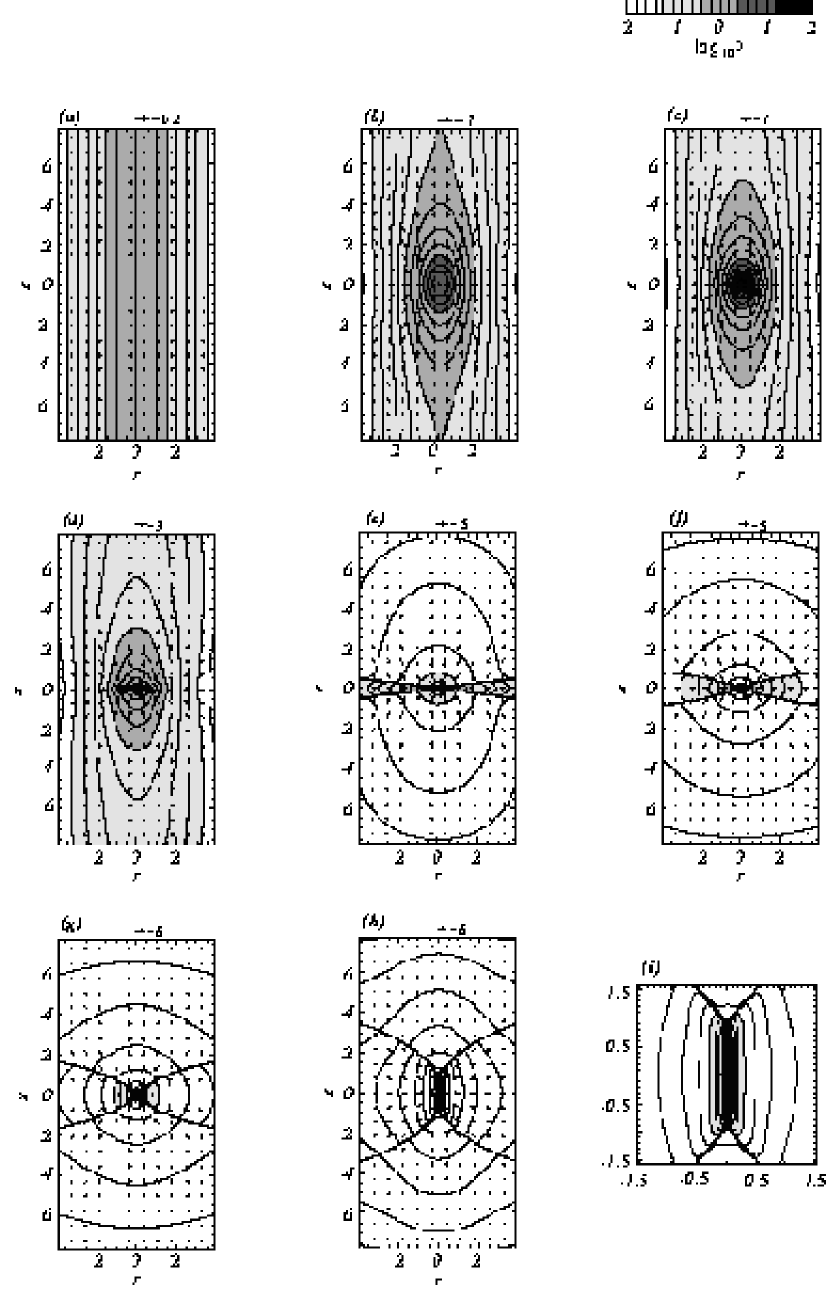
Figure 1: Density and velocity distributions in the $r-z$ plane for model B at eight different stages. This model has the initial parameters of $\beta=0$ and $\lambda_{z}=15.5r_{\rm u}$. The gray scale indicates the density distribution in a logarithmic scale. The arrows show the velocity distributions which are normalized separately in each panel. Panels (a) through (h) show the cross sections at (a) $t-t_{\rm core}=-7.23t_{\rm u}$ ($\rho_{c}=\rho_{0}$), (b) $-0.59$ ($\rho_{c}=10\rho_{0}$), (c) 0.00 ($\rho_{c}=10^{4}\rho_{0}$), (d) 0.93 ($M_{0}\simeq 0.3M_{\rm t}$), (e) 2.25 ($M_{0}\simeq 0.5M_{\rm t}$), (f) 4.49 ($M_{0}\simeq 0.7M_{\rm t}$), (g) 8.28 ($M_{0}\simeq 0.86M_{\rm t}$), and (h) 10.88 ($M_{0}\simeq 0.9M_{\rm t}$), respectively, where $t-t_{\rm core}$ is the time measured from the epoch of core formation, $\rho_{c}$ is the central density, and $M_{\rm 0}$ is the mass of the central point-like object. The first three panels represent the cross sections during the runaway collapse phase, while the others are during the accretion phase. Panel (i) denotes the enlargement of the central region of panel (h). If we adopt $\rho_{0}=10^{6}$cm^-3 and $c_{s}=0.2$km s^-1, then the units of time, length, and mass are given as $t_{\rm u}=(2\pi G\rho_{0})^{-0.5}=2.5\times 10^{4}$ yr, $r_{\rm u}=c_{s}t_{\rm u}=1.1\times 10^{3}$ AU, and $m_{\rm u}=\rho_{0}r_{\rm u}^{3}=7.6\times 10^{-3}M_{\odot}$, respectively. The total cloud mass is equal to $1.9\times 10^{2}m_{\rm u}=1.5M_{\odot}$.

Figure 1 shows the density and velocity distributions in the $r-z$ plane at eight different stages. The first three panels show the cross sections of the cloud during the runaway collapse phase, while the others show those during the accretion phase. At the early stages, the cloud collapses preferentially towards the $z=0$ plane (Figs. 1b and 1c). As the collapse proceeds, the central high-density region becomes spherical, whereas the low-density region remains prolate. The central spherical region continues to contract towards the center. Such evolution is the same as that of model D by Nakamura et al. (1995).

When the central density reaches $10^{4}\rho_{0}$, the sink cell method is applied and the central point-like object forms. The mass of the central point-like object monotonously increases with time. Since the vertical flow is dominant near the center, the disklike envelope is formed around the central point-like object and grows in radial extent (Figs. 1d and 1e). A shock wave is also formed at the disk surface. By the stage at which the mass of the central point-like object reaches about $0.7M_{\rm t}$, the infalling disk extends radially up to $r\sim 4-5r_{\rm u}$, where $M_{\rm t}$ denotes the total cloud mass. In the disk, the gravitational force dominates the pressure force in the radial direction, while in the vertical direction, the pressure force becomes comparable to the gravitational force. Therefore, the gas flow progresses mainly in the radial direction inside the disk. Such an non-equilibrium disk resembles pseudo-disks found by Galli & Shu (1993), Hartmann et al. (1994), and Bonnell et al. (1996).

After the mass of the central point-like object reaches about $0.7M_{\rm t}$, the radius of the infalling disk becomes shorter because of dominant radial infall (Figs. 1f and 1g). The shock front lifts up vertically because of dominant pressure force in the vertical direction. Thereafter, the shock front reaches the $z$-axis and thus the matter in the infalling disk collapses to form a thin needle-like (prolate) object along the $z$-axis (Figs. 1h and 1i).

We also followed the evolution of models A and C to examine the effects of $\lambda$ on the formation and evolution of the disklike envelope. It is found that the evolution is qualitatively similar to that of model B. In both models, the disklike envelopes are formed and then they evolve into thin needle-like objects. For the model with larger $\lambda$, the vertical infall is more dominant and thus the disk is more extended in the radial direction.

3.2 Prolate Cloud Cores with Slow Rotation

In this subsection, we explore the evolution of slowly-rotating clouds. In the following, we mainly show the numerical results of model E as a typical example. In this model, the wavelength $\lambda_{z}$ is almost equal to that of the fastest growing linear perturbation. As shown below, the evolution of model E is qualitatively similar to that of model B except near the center, i.e., the cloud collapses to form an infalling disk in which the gas flows mainly in the radial direction.

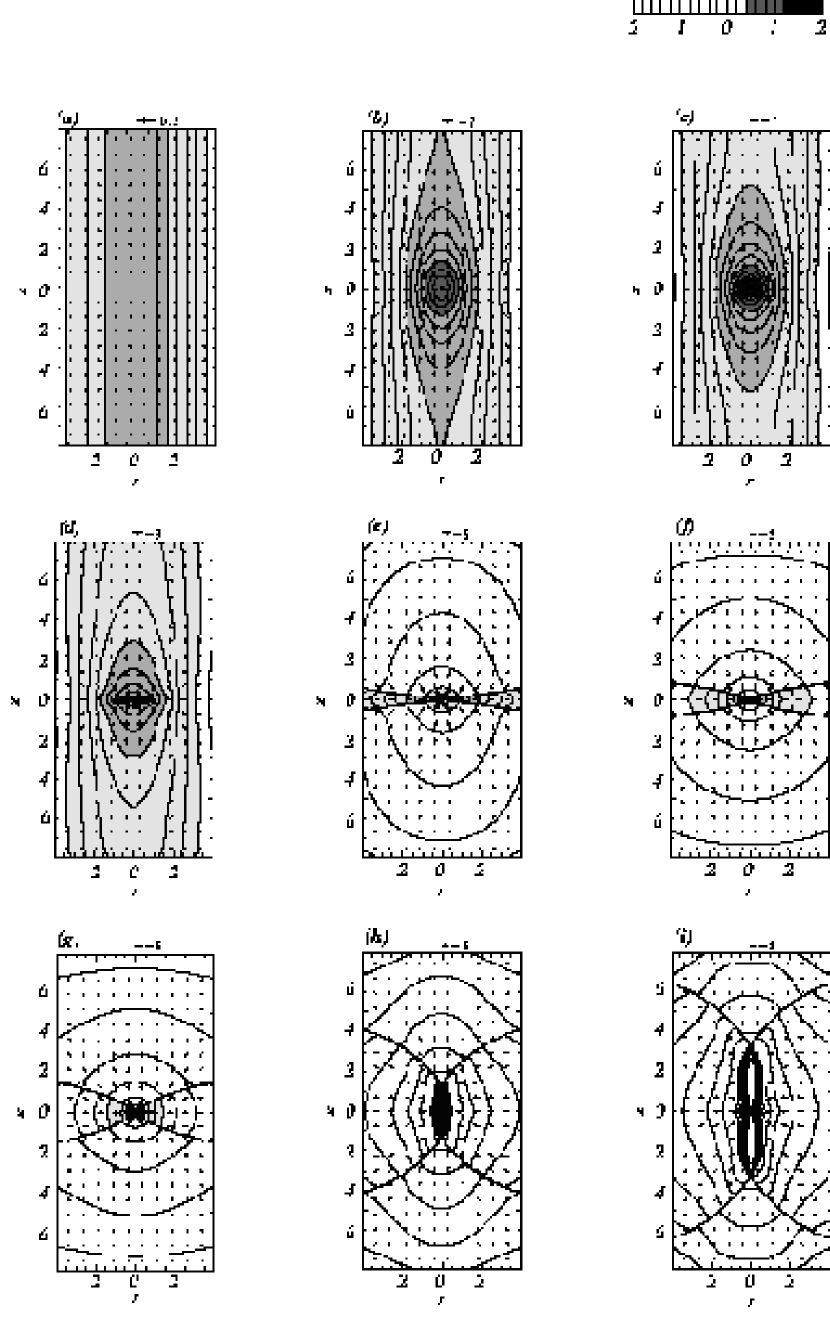
Figure 2: Same as Figure 1 but for model E. This model has the initial parameters of $\beta=0.05$ and $\lambda_{z}=15.5r_{\rm u}$. Panels (a) through (i) show the cross sections at (a) $t-t_{\rm core}=-7.26t_{\rm u}$ ($\rho_{c}=\rho_{0}$), (b) $-0.59$ ($\rho_{c}=10\rho_{0}$), (c) 0.00 ($\rho_{c}=10^{4}\rho_{0}$), (d) 0.98 ($M_{0}\simeq 0.3M_{\rm t}$), (e) 4.71 ($M_{0}\simeq 0.7M_{\rm t}$), (f) 6.59 ($M_{0}\simeq 0.79M_{\rm t}$), (g) 8.25 ($M_{0}\simeq 0.82M_{\rm t}$), (h) 11.74 ($M_{0}\simeq 0.84M_{\rm t}$),and (i) 13.44 ($M_{0}\simeq 0.85M_{\rm t}$), respectively, where $t-t_{\rm core}$ is the time measured from the epoch of core formation, $\rho_{c}$ is the central density, and $M_{\rm 0}$ is the mass of the central point-like object. If we adopt $\rho_{0}=10^{6}$cm^-3 and $c_{s}=0.2$km s^-1, then the units of time, length, and mass are given as $t_{\rm u}=(2\pi G\rho_{0})^{-0.5}=2.5\times 10^{4}$ yr, $r_{\rm u}=c_{s}t_{\rm u}=1.1\times 10^{3}$ AU, and $m_{\rm u}=\rho_{0}r_{\rm u}^{3}=7.6\times 10^{-3}M_{\odot}$, respectively. The total cloud mass is equal to $2.1\times 10^{2}m_{\rm u}=1.6M_{\odot}$.

Figure 2 is the same as Figure 1 but for model E. During the runaway collapse phase, the central high-density region becomes slightly oblate because of rotation, whereas the low-density region remains prolate. In the central region, the rotation is not important in the cloud support. Therefore, the central region continues to contract.

After the central core is formed, the disklike envelope is formed and then expands in radius (Figs. 2d and 2e). A shock wave is also formed at the disk surface and propagates towards the $z$-axis. Such evolution is essentially the same as that of model B. In the disk, the rotation is not important and therefore the gas flow progresses primarily in the radial direction. As the contraction proceeds, the centrifugal force becomes important at the innermost region and a rotationally-supported disk is formed there.

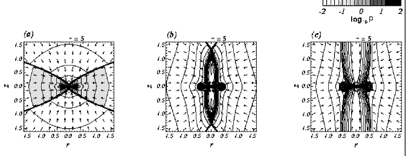
Figure 3: Density and velocity distributions of the central region for model E. Panels (a), (b), and (c) denote the cross sections at the same stages as panels (g), (h), and (i) of Figure 2, respectively. [(a) $t-t_{\rm core}=8.25t_{\rm u}$ ($M_{0}\simeq 0.82M_{\rm t}$), (b) 11.74 ($M_{0}\simeq 0.84M_{\rm t}$), and (c) 13.44 ($M_{0}\simeq 0.85M_{\rm t}$), respectively, where $t-t_{\rm core}$ is the time measured from the epoch of core formation and $M_{\rm 0}$ is the mass of the central point-like object.]

After the mass of the central region reaches about $0.7M_{\rm t}$, the radius of the infalling disk becomes shorter owing to dominant radial infall (Figs. 2f and 2g). Then, the matter in the infalling disk collapses to form a funnel in which the centrifugal force balances with the gravitational force in the radial direction (Figs. 2h and 2i). In Figure 3, we show the enlargements of the central region at the same stages as the last three panels of Figure 2. A new shock front is also formed there and propagates in the radial direction as the gas with higher specific angular momentum accretes. Such a structure resembles a bipolar cavity which is often thought to be formed by the outflow from the central young star. This structure might play a significant role in the guidance of outflow from the central star at the late stages of the evolution.

The rotationally-supported disk is encased in two accretion shock fronts, both of which are located several scale heights above the equatorial plane (Figs. 3b and 3c). Such structure seems to be similar to that of Yorke & Bodenheimer (1999). Shock formation is explained as follows. In the infalling disk, the accretion flow is dominant in the radial direction. The radial infall stops at the funnel owing to the centrifugal barrier and thus the outer shock front is formed. Thereafter, the matter in the rotationally-supported disk collapses in the vertical direction to achieve hydrostatic equilibrium. This infall produces the inner shock front. In the innermost disk, angular momentum transfer is expected to be important in the accretion flow onto the central core, although it is not included in the present calculations (see Yorke & Bodenheimer 1999).

We also pursued the evolution of models D and F to examine the effects of $\beta$. It is found that the evolution is qualitatively similar to that of model E, although the size of the rotationally-supported disk depends on $\beta$, i.e., when $\beta$ is larger, the rotatinally-supported disk is wider.

3.3 Effects of Cloud Geometry (Prolate vs. Oblate Cloud Cores)

As shown in §3.1 and §3.2, a prolate cloud core collapses to form an infalling disk in which the accreting gas flows mainly in the radial direction. In this subsection, to clarify the physics of the formation process of the infalling disk, we calculate the evolution of two representative models: (1) a prolate cloud and (2) an oblate cloud. In the following, we consider non-rotating prolate and oblate clouds which have Gaussian-like density profiles as

$$\rho=\rho_{0}\exp\left[-\left(\frac{r^{2}}{R_{0}^{2}}+\frac{z^{2}}{Z_{0}^{2}}\right)\right]\;.$$ (7)

At the initial state, the cloud is assumed to be static for simplicity. This model has the two parameters of $R_{0}$ and $Z_{0}$.

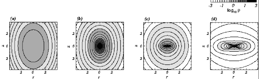
Figure 4: Density and velocity distributions in the $r-z$ plane for the prolate cloud at four different stages. This model has the initial parameters of $(R_{0},Z_{0})=(1.66r_{\rm u},2.49r_{\rm u})$. The gray scale indicates the density distribution in a logarithmic scale. Panels (a) through (d) show the cross sections at (a) $t-t_{\rm core}=-2.06t_{\rm u}$ ($\rho_{c}=\rho_{0}$), (b) 0.00 ($\rho_{c}=10^{4}\rho_{0}$), (c) 1.09 ($M_{0}\simeq 0.5M_{\rm t}$), (d) 2.64 ($M_{0}\simeq 0.7M_{\rm t}$), respectively, where $t-t_{\rm core}$ is the time measured from the epoch of core formation, $\rho_{c}$ is the central density, and $M_{\rm 0}$ is the mass of the central point-like object.

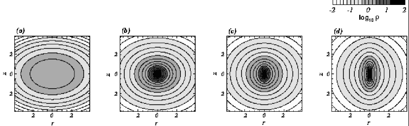
Figure 5: Same as Figure 4 but for the oblate cloud. This model has the initial parameters of $(R_{0},Z_{0})=(2.40r_{\rm u},1.60r_{\rm u})$. The gray scale indicates the density distribution in a logarithmic scale. Panels (a) through (d) show the cross sections at (a) $t-t_{\rm core}=-2.08t_{\rm u}$ ($\rho_{c}=\rho_{0}$), (b) 0.00 ($\rho_{c}=10^{4}\rho_{0}$), (c) 0.49 ($M_{0}\simeq 0.3M_{\rm t}$), (d) 1.12 ($M_{0}\simeq 0.5M_{\rm t}$), respectively, where $t-t_{\rm core}$ is the time measured from the epoch of core formation, $\rho_{c}$ is the central density, and $M_{\rm 0}$ is the mass of the central point-like object.

Figures 4 and 5 show the evolutions of the density distributions in the $r-z$ plane for the prolate and oblate clouds, respectively. The prolate and oblate clouds have the model parameters of $(R_{0},Z_{0})=(1.66r_{\rm u},2.49r_{\rm u})$ and $(2.40r_{\rm u},1.60r_{\rm u})$, respectively. In both models, the ratio of the major to minor axes is set to 1.5 and the ratio of the thermal energy to the gravitational energy is equal to $\alpha\sim 0.33$. The total cloud masses are equal to $M_{\rm t}=1.44\times 10^{2}m_{\rm u}$ and $1.40\times 10^{2}m_{\rm u}$ for the prolate and oblate clouds, respectively. The grid spacing is set to $\Delta r=\Delta z=0.02r_{u}$. The number of grid points is taken to be $N_{r}\times N_{z}=512\times 1024$ In Figures 4 and 5, the first two panels show the cross sections during the runaway collapse phase, while the rest are during the accretion phase. In both models, the contraction progresses preferentially along the major axis. Therefore, during the accretion phase, the initially prolate cloud collapses into an oblate core, whereas the initially oblate cloud collapses into a prolate core.

This evolution is explained as follows. At the initial state, the pressure force is less effective along the major axis because of shallower density gradient. In other words, the net attractive force is stronger along the major axis. Therefore, the cloud collapses preferentially along the major axis.

We also followed the evolution of the models with different axis ratios and $\alpha$. It is found that as long as the cloud is close to virial equilibrium, the evolution is qualitatively similar to those shown here (see also Bonnell et al. 1996).

As mentioned in §2, the fragments formed from filamentary clouds tend to become prolate at the epoch of fragmentation. Therefore, as shown in §3.1 and §3.2, such a prolate fragment collapses to form an oblate core which thereafter evolves into a prolate core. This evolution is consistent with those of Figures 4 and 5.

4 Time-Dependent Mass Infall Rate

In this section, we discuss the evolution of the mass infall rate onto the center.

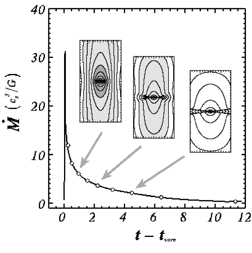
Figure 6: Mass infall rate of model B as a function of time measured from the epoch of core formation ($t-t_{\rm core}$). If we adopt $\rho_{0}=10^{6}$cm^-3 and $c_{s}=0.2$km s^-1, then the units of time and mass infall rate are given as $t_{\rm u}=(2\pi G\rho_{0})^{-0.5}=2.5\times 10^{4}$ yr and $c_{s}^{3}/G=1.9\times 10^{-6}M_{\odot}$ yr^-1, respectively. Open circles denote the stages at which $M_{0}=0.1M_{\rm t}$, $0.2M_{\rm t}$, $\cdots$, $0.7M_{\rm t}$. For comparison, we show the cross sections of the cloud at the stages of $M_{0}=0.3M_{\rm t}$, 0.5 $M_{\rm t}$, and 0.7 $M_{\rm t}$.

Figure 6 shows the evolution of the mass infall rate for model B. The mass infall rate is time-dependent, in contrast to the prediction of similarity solutions (e.g., Shu 1977; Whitworth & Summers 1985). The mass infall rate takes its maximum at the very early stage and then monotonously decreases with time. This behavior is basically the same as that of Ogino, Tomisaka, Nakamura (1999)’s model with a small $\alpha$, where $\alpha$ is the ratio of the gravitational force to the pressure force. Such evolution is explained as follows. During the runaway collapse phase, the central region tends to approach the Larson-Penston similarity solution (Larson 1969; Penston 1969) whose mass infall rate is temporally constant at $\dot{M}_{\rm LP}\sim 47c_{s}^{3}/G$. However, only the central small region converges onto the Larson-Penston solution by the epoch of core formation. In the outer infalling envelope, the pressure effect is important and the infall is appreciably retarded. Thus, after the central small region accretes onto the central point mass, the mass infall rate declines in time.

Observed young stellar objects (YSOs) are often classified into several empirical evolutional stages from star-less dense cores to main-sequence stars (e.g., André, Ward-Thompson, & Barsony 1993). The youngest observed YSOs are called Class 0 sources which are interpreted to be in a phase at which the envelope gas still has more mass than the central hydrostatic protostellar core. More evolved YSOs are called Class I sources. Recently, Bontemps et al. (1996) suggested that if the CO outflow rates are proportional to the mass infall rates onto the embedded young stars, the mass infall rates of Class 0 sources are a factor of 10 larger on average than those of Class I sources. Applying a simplified pressure-free model, Henriksen, André, & Bontemps (1997) proposed that the observed dispersion of the mass infall rates for Class 0 sources is due to the time evolution of the mass infall rates. In our isothermal model, the evolution of the mass infall rate is qualitatively similar to that of Henriksen et al. (1997), although in our hydrodynamical model, the pressure force significantly retards the rapid change of the mass infall rate. As discussed by Ogino et al. (1999), the evolution of the mass infall rate also depends on the initial conditions of the clouds. We will discuss those effects in a separate paper.

5 Implications to Observations

Recent observations have revealed the detailed structures of the infalling envelopes around several embedded young stars (e.g., Hayashi et al. 1993; Ohashi et al. 1996; Saito et al. 1996; Momose et al. 1996). In this section, we discuss the physical structures of the disklike envelopes obtained by our calculations and make a comparison between our numerical results and observations.

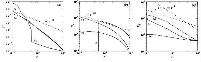
Figure 7: Radial profiles of (a) density, (b) radial velocity, and (c) azimuthal velocity in the equatorial plane for model E. They are plotted at the stages at which (1) $t-t_{\rm core}=0.00t_{\rm u}$ (the epoch of core formation), (2) 1.56 ($M_{0}\simeq 0.4M_{\rm t}$), and (3) 13.43 ($M_{0}\simeq 0.85M_{\rm t}$), where $t-t_{\rm core}$ is the time measured from the epoch of core formation and $M_{\rm 0}$ is the mass of the central point-like object. If we adopt $\rho_{0}=10^{6}$cm^-3 and $c_{s}=0.2$km s^-1, then the units of time and length are given as $t_{\rm u}=(2\pi G\rho_{0})^{-0.5}=2.5\times 10^{4}$ yr and $r_{\rm u}=c_{s}t_{\rm u}=1.1\times 10^{3}$ AU, respectively. The total cloud mass is equal to $2.1\times 10^{2}m_{\rm u}=1.6M_{\odot}$.

Figure 7 shows the radial profiles of $\rho$, $v_{r}$, and $v_{\varphi}$ in the equatorial plane during the accretion phase. Just after core formation, the density and velocity profiles are well approximated by $\rho\propto r^{-2}$, $v_{r}\sim{\rm const.}$, and $v_{\varphi}\sim{\rm const.}$ near the center. This indicates that the central high-density region converges well onto a similarity solution by the epoch of core formation (Matsumoto et al. 1997). As the collapse progresses, both the infalling disk and the rotationally-supported disk grow in size. In the infalling disk, the density, radial velocity, and azimuthal velocity have the radial distributions of $\rho\propto r^{-1.5}$, $v_{r}\propto r^{-0.5}$, and $v_{\varphi}\propto r^{-1}$, respectively. The radial velocity is reproduced by a free-fall velocity of $\sqrt{2GM_{0}/r}$. The azimuthal velocity means that the specific angular momentum is almost constant in the infalling envelope. Such dependence seems to be qualitatively similar to that of a similarity solution of an infalling rotating disk (Saigo & Hanawa 1998; see also Terebey, Shu, Cassen 1984). In the rotationally-supported disk, the radial and azimuthal velocities are well approximated by $v_{r}\sim 0$ and $v_{\varphi}\propto r^{-0.5}$, respectively. At the boundary between the infalling disk and the rotationally-supported disk, a shock wave is formed and propagates outwardly.

Momose et al. (1996) have examined the physical structure of the infalling disk around the L1551 IRS5. From a comparison between the observed postion-velocity diagram and their simple analytic model, they suggested that the velocity field in the disklike envelope is explained in terms of infall with slow rotation. Their simple model indicates that the infall and azimuthal velocities have radial dependences of $v_{r}\propto r^{-0.5}$ with 0.5 km s^-1 at $r=700$ AU and $v_{\varphi}\propto r^{-1}$ with 0.24 km s^-1 at $r=700$ AU, respectively. If we take $\rho_{0}\sim 10^{6}$ cm^-3 and $T=10$ K, then the observed velocity field around the L1551 IRS5 is consistent with that of the model presented in §3.2 at the stage at which $t-t_{\rm core}\sim 1.5(2\pi G\rho_{0})^{-0.5}\simeq 3.8\times 10^{4}$ yr, where $t-t_{\rm core}$ denotes the time measured from the epoch of core formation. The mass infall rate is evaluated as $\dot{M}\sim 1\times 10^{-5}M_{\odot}$ yr^-1. The central mass (a point mass plus its surrounding rotationally-supported disk) is then estimated as 0.6 $M_{\odot}$.

The detailed comparisons between the numerical results and observations will reveal the formation and evolution processes of the infalling envelopes as well as the young stars.

Table 1: MODEL PARAMETERS

Model	$\beta$	$\lambda_{z}$	$M_{\rm t}$	$\Delta r=\Delta z$	$N_{r}\times N_{z}$
A	0	10.4	$1.25\times 10^{2}$	$1.01\times 10^{-2}$	$1024\times 512$
B	0	15.5	$1.93\times 10^{2}$	$1.52\times 10^{-2}$	$1024\times 512$
C	0	23.3	$2.91\times 10^{2}$	$2.27\times 10^{-2}$	$1024\times 512$
D	0.01	15.5	$1.93\times 10^{2}$	$1.52\times 10^{-2}$	$1024\times 512$
E	0.05	15.5	$2.07\times 10^{2}$	$1.52\times 10^{-2}$	$1024\times 512$
F	0.10	15.5	$2.10\times 10^{2}$	$1.52\times 10^{-2}$	$1024\times 512$

Note. — $\beta=$ the ratio of the centrifugal force to the pressure force; $\lambda_{z}=$ the longitudinal wavelength; $M_{\rm t}=$ total cloud mass; $\Delta r$ and $\Delta z=$ the grid spacings in the $r$- and $z$-directions; $N_{r}$ and $N_{z}=$ the number of grid points in the $r$- and $z$-directions.

References

- André et al. (1993) André, P., Ward-Thompson, D., & Barsony, M. 1993, ApJ, 406, 122
- Bonnell et al. (1996) Bonnell, I., Bate, M. R., & Price, N. M. 1996, MNRAS, 279, 121
- Bontemps et al. (1996) Bontemps S., André P., Terebey S., & Cabrit S. 1996, A&A, 311, 858
- Boss (1987) Boss, A. P., 1987, ApJ, 316, 721
- Boss & Black (1982) Boss, A. P., & Black, D.C. 1982, ApJ, 258, 270
- Goodman et al. (1993) Goodman, A., Benson, P., Fuller, G., & Myers, P. 1993, ApJ, 406, 528
- Galli & Shu (1993) Galli, D., & Shu, F. H. 1993, ApJ, 417, 243
- Hartmann et al. (1994) Hartmann, L., Boss, A., Calvet, N., & Whitney, B. 1994, ApJ, 430, L52
- Hayashi et al. (1993) Hayashi, M., Ohashi, N., & Miyama, S. M. 1993, ApJ, 418, L71
- Henriksen et al. (1997) Henriksen R., André P., & Bontemps S. 1997, A&A, 323, 549
- Klessen et al. (1998) Klessen, R. S., Burkert, A., & Bate, M. S. 1998, ApJ, 501, L205
- Larson (1969) Larson, R. B. 1969, MNRAS, 145, 271
- Matsumoto et al. (1994) Matsumoto, T., Nakamura, F., & Hanawa, T. 1994, PASJ, 46, 243
- Matsumoto et al. (1997) Matsumoto, T., Hanawa, T., & Nakamura, F. 1997, ApJ, 478, 569
- Momose et al. (1996) Momose, M., Ohashi, N., Kawabe, R., Hayashi, M., & Nakano, T. 1996, ApJ, 470, 1001
- Myers et al. (1991) Myers, P. C., Fuller, G. A., Goodman, A. A., & Benson, P. J. 1991, ApJ, 376, 561
- Nakamura et al. (1995) Nakamura, F., Hanawa, T., & Nakano, T. 1995, ApJ, 444, 770
- Nakamura et al. (1993) Nakamura, F., Hanawa, T., & Nakano, T. 1993, PASJ, 45, 551
- Ogino et al. (1999) Ogino, S., Tomisaka, K., & Nakamura, F. 1999, PASJ, 51, 637
- Ohashi et al. (1996) Ohashi, N., Hayashi, M., Ho, P., Momose, M., & Hirano, N. 1996, ApJ, 466, 957
- Penston (1969) Penston, M. V. 1969, MNRAS, 144, 425
- Sago & Hanawa (1998) Saigo, K., & Hanawa, T. 1998, ApJ, 493, 342
- Saito et al. (1996) Saito, M., Kawabe, R., Kitamura, Y., & Sunada, K. 1996, ApJ, 473, 464
- Shu (1977) Shu, F. H. 1977, ApJ, 214, 488
- Terebey et al. (1984) Terebey, S., Shu, F. H, & Cassen, P. 1984, ApJ, 286, 529
- Tomisaka (1996) Tomisaka, K. 1996, PASJ, 48, L97
- Whitworth & Summers (1985) Whitworth, A., & Summers, D. 1985, MNRAS, 214, 1
- Yorke & Bodenheimer (1999) Yorke, H. W., & Bodenheimer, P. 1999, ApJ, 525, 330