The ATESP Radio Survey

Abstract

This paper is the first of a series reporting the results of the Australia Telescope ESO Slice Project (ATESP) radio survey obtained at 1400 MHz with the Australia Telescope Compact Array (ATCA) close to the South Galactic Pole (SGP) over the region covered by the ESO Slice Project (ESP) galaxy redshift survey ($\delta\sim-40\degr$). The survey consists of 16 radio mosaics with $\sim 8\arcsec\times 14\arcsec$ resolution and uniform sensitivity ($1\sigma$ noise level $\sim$79 $\mu$Jy) over an area of $\sim 26$ sq. degrees. Here we present the design of the survey, we describe the mosaic observing technique which was used to obtain an optimal combination of uniform and high sensitivity over the whole area, and the data reduction: the problems encountered and the solutions adopted.

1 Introduction

Sky surveys play an important role in astronomy. Large collections of objects allow reliable studies of the average properties of different constituents of the universe; new populations can be found and well defined sub-samples can be extracted for further detailed analysis.
Surveys in the radio domain have yielded many important results in the past, since the discovery of radio galaxies and quasars. The first samples of radio sources ($S\ga 1$ Jy) have demonstrated that classical radio galaxies are rare in the local universe and strongly evolve with cosmic time both in density and luminosity (e.g. Longair Longair66 (1966)). More recently, deep radio surveys ($S\la 1$ mJy) have shown that normalized radio counts show a flattening below a few mJy, corresponding to a steepening in the actual observed counts (see e.g. Windhorst et al. Windhorst90 (1990) for counts at 1.4 GHz). This change of slope is generally interpreted as being due to the presence of a new population of radio sources (the so-called sub-mJy population) which does not show up at higher flux densities (see e.g. Condon Condon89 (1989)). To explain the new faint radio population several scenarios have been invoked: strongly-evolving normal spirals (Condon Condon84 (1984), Condon89 (1989)); actively star forming galaxies (e.g. Rowan-Robinson et al. Rowan93 (1993)); or a non-evolving population of local (z $<$ 0.1) low-luminosity galaxies (e.g. Wall et al. Wall86 (1986)). The true nature of the population is not well established. The same is true for the relative contributions from the above mentioned objects. Furthermore the source space density inferred from the faint end of the local bivariate luminosity function for both spirals and ellipticals is not well known (see e.g. Condon Condon96 (1996)). Therefore it is not possible to estimate the local contribution to the counts (even if expected to be small) nor is there a clear local reference frame for understanding evolutionary phenomena.
Unfortunately, due to the long observing times required to reach faint fluxes, the existing samples in the sub-mJy region are generally small. Table 1 shows a compilation of the largest 1.4 GHz surveys available in the mJy and sub-mJy regime with the surveyed areas and limiting fluxes (note, however, that the quoted limiting fluxes are often not uniform over the entire areas).
The identification work and subsequent spectroscopy are very demanding in terms of telescope time. Typically, no more than $\sim 50-60\%$ of the radio sources in sub-mJy samples have been identified on optical images, even though for the $\mu$Jy survey in the Hubble Deep Field an identification rate of about 80$\%$ has been reached (Richards et al. Richards99 (1999)). On the other hand, the typical fraction of spectra available is only $\sim 20\%$. The best studied sample is the Marano Field, where $\sim 45\%$ of the sources have spectral information (Gruppioni et al. 1999a ).
To establish a firm point in the radio properties of galaxies in the local (z $<$ 0.2) universe it is necessary to survey a large area in the sky down to faint flux limits. Furthermore it is necessary to have in the same region a statistically significant sample of galaxies with well studied optical properties (radial velocities, magnitudes etc.). To alleviate the identification work, regions with deep photometry (possibly multicolor) already available provide a significant advantage. The region we have selected fulfills these requirements at least partially.
Vettolani et al. (Vettolani97 (1997)) made a deep redshift survey in two strips of $22^{\circ}\times 1^{\circ}$ and $5^{\circ}\times 1^{\circ}$ near the SGP by studying photometrically and spectroscopically nearly all galaxies down to $b_{J}\sim$ 19.4. The survey, yielding 3342 redshifts (Vettolani et al. Vettolani98 (1998)), has a typical depth of $z=0.1$ with 10$\%$ of the objects at $z>0.2$ and is $90\%$ complete. In the same region lies the ESO Imaging Survey (EIS, Nonino et al. Nonino99 (1999)) Patch A (3.2 sq. degr.), consisting of deep images in the I band out of which a galaxy catalogue $95\%$ complete to $I=22.5$ has been extracted. Further V band images are available over $\sim$ 1.5 sq. degr.
We used the 6 km configuration of the ATCA to make a 20 cm radio continuum mosaic of the region covered by the ESP galaxy redshift survey. The ATESP radio survey has uniform sensitivity ($1\sigma$ noise level $\sim$79 $\mu$Jy).

The present paper essentially deals with a description of the survey, the observations, the mosaic technique and the data reduction. It is organized as follows. In Sect. 2 the survey design, in particular with respect to the mosaic technique is explained. In Sects. 3 and 4 we present in detail the calibration of our 20 cm observations and the data reduction. We discuss the problems encountered and the solutions adopted. Sect. 5 is dedicated to the analysis of the mosaics. A summary is given in Sect. 6.

Table 1: 1.4 GHz mJy and sub-mJy radio surveys.

Survey	References	Area	$S_{lim}$
		sq. deg.	mJy
NVSS	Condon et al. Condon98 (1998)	3 $\times 10^{4}$	2.5
ELAIS N b	Ciliegi et al. Ciliegi99 (1999)	4.22	1.15
FIRST	White et al. White97 (1997)	1550	1.0
ELAIS S	Gruppioni et al. 1999b	4.0	0.4
VLA-NEP	Kollgaard et al. Kollg94 (1994)	29.3	0.3
PDF	Hopkins et al. Hopkins98 (1998)	3.0	0.2
Marano Field	Gruppioni et al. Gruppioni97 (1997)	0.36	0.2
ELAIS N a	Ciliegi et al. Ciliegi99 (1999)	0.12	0.135
LBDS	Windhorst et al. Windhorst84 (1984)	5.5	0.1 - 0.2
Lockman Hole	de Ruiter et al. Ruiter97 (1997)	0.35	0.12
Lynx 3A	Oort Oort87 (1987)	0.8	0.1
0852+17	Condon & Mitchell CM84 (1984)	0.32	0.08
1300+30	Mitchell & Condon MC85 (1985)	0.25	0.08
HDF	Richards Richards99a (1999)	0.3	0.04
ATESP	this paper	25.9	0.47

2 Survey design

The radio observations were carried out with two main goals in mind. The first aim was to detect the ESP galaxies in order to derive the ‘local’ ($z\sim 0.1$) bivariate luminosity function. We therefore tried to keep the sensitivity as uniform as possible over the whole ESP area, while at the same time reaching flux densities well below $\sim 1$ mJy (see Sect. 2.2).
The second aim was to have a complete catalogue of faint radio sources in order to study the sub-mJy population through a programme of optical identification of complete radio source samples extracted from the ATESP survey, exploiting the available data, i.e. deep CCD images.
As the survey is intended to achieve uniform sensitivity over a large area it is necessary to make use of the mosaicing technique.

2.1 Mosaicing Technique

Mosaicing is the combination of regularly spaced multiple pointings of a radio telescope which are then linearly combined to produce an image larger than the radio telescope’s primary beam. The linear mosaicing consists of a weighted average of the pixels in the individual pointings, with the weights determined by the primary beam response and the expected noise level (see equation in Sault & Killeen SK95 (1995)). If the observing parameters and conditions are the same for every individual pointing, the expected noise variance in any observed field can be assumed to be equal for every observing field and the intensity distribution in the mosaiced final image, $I(l,m)$, is modulated only by the primary beam response:

$$I(l,m)=\frac{\sum_{i}P(l-l_{i},m-m_{i})I_{i}(l,m)}{\sum_{i}P^{2}(l-l_{i},m-m_{i})}$$ (1)

where the summation is over the set of pointing centres $(l_{i},m_{i})$. $I_{i}(l,m)$ is the image formed from the $i$-th pointing (not corrected for the primary beam response) and $P(l,m)$ is the primary beam pattern.
In planning a mosaicing experiment, the main issue to be decided is the pointing grid pattern, i.e. geometry and pointing spacings. For a detection experiment on a large area of sky (like the ATESP survey) the main requirement is uniform sensitivity over the entire region together with high observing efficiency. Such requirement can be satisfied by choosing opportunely the pointing grid pattern.
The mosaic noise standard deviation, $\sigma(I(l,m))$, can be obtained from the error propagation of Eq. 1 and the uniform sensitivity constraint is expressed by

$$\frac{\sigma(I(l,m))}{\sigma}=\frac{1}{\sqrt{\sum_{i}P_{i}^{2}(l-l_{i},m-m_{i})}}=constant$$ (2)

for every position $(l,m)$. In other words, the mosaic sensitivity, expressed in terms of $\sigma$s ($\sigma$ is the noise expected in the individual pointings) is modulated by the squared sum of the primary beam response.
The ATCA primary beam pattern can be approximated by a circular Gaussian function (Wieringa & Kesteven Wieringa92 (1992))

$$P_{i}(r)=\mathrm{e}^{-4\ln 2\left(\frac{r}{\mbox{FWHP}}\right)^{2}},$$ (3)

where $r=\sqrt{l^{2}+m^{2}}$ is the radial distance from the image phase center and FWHP is the full width at half power of the primary beam ($\sim$ 33 arcmin for ATCA observations at 1.4 GHz). Since the square of a Gaussian is still a Gaussian with FWHP reduced by a factor $\sqrt{2}$, the quadratic sum in Eq. 2 can be written as a linear sum of Gaussians with FWHP$\arcmin=\mbox{FWHP}/\sqrt{2}$ (corresponding to $s\simeq 33\arcmin/\sqrt{2}=23.3\arcmin$ for ATCA 1.4 GHz observations).
To make the final choice for the ATESP survey grid pattern, we have performed a series of simulations of the bidimensional quantity

$$\sigma(I)/\sigma=\frac{1}{\sqrt{\sum_{i}\mbox{e}^{-4\ln 2\left(\frac{(s_{i}-r)}{\mbox{FWHP}\arcmin}\right)^{2}}}}$$ (4)

where $s_{i}=(l_{i},m_{i})$, $r=\sqrt{(l-l_{i})^{2}+(m-m_{i})^{2}}$ and FWHP$\arcmin=23.3\arcmin$, varying the pointing spacings $s$ and the grid geometry (hexagonal and/or rectangular grids).
In general a very good compromise between uniform sensitivity and observing efficiency is represented by a grid pattern with pointing spacings of the order of $s\simeq\mbox{FWHP}\arcmin$. For our particular case, the best choice turned out to be a $20\arcmin$ spacing rectangular grid. The mosaic noise variations over a reference area of 1 sq. degr. for such a grid configuration are shown in Fig. 1. As expected, in the region of interest (central box) the noise is rather constant: variations are $\leq 5\%$, except at the region borders ($\leq 10\%$). We point out that hexagonal grids should be preferred when imaging wide areas of sky (like for the NVSS and FIRST radio surveys), but are not very efficient in the case of a narrow 1-degree wide strip of sky.

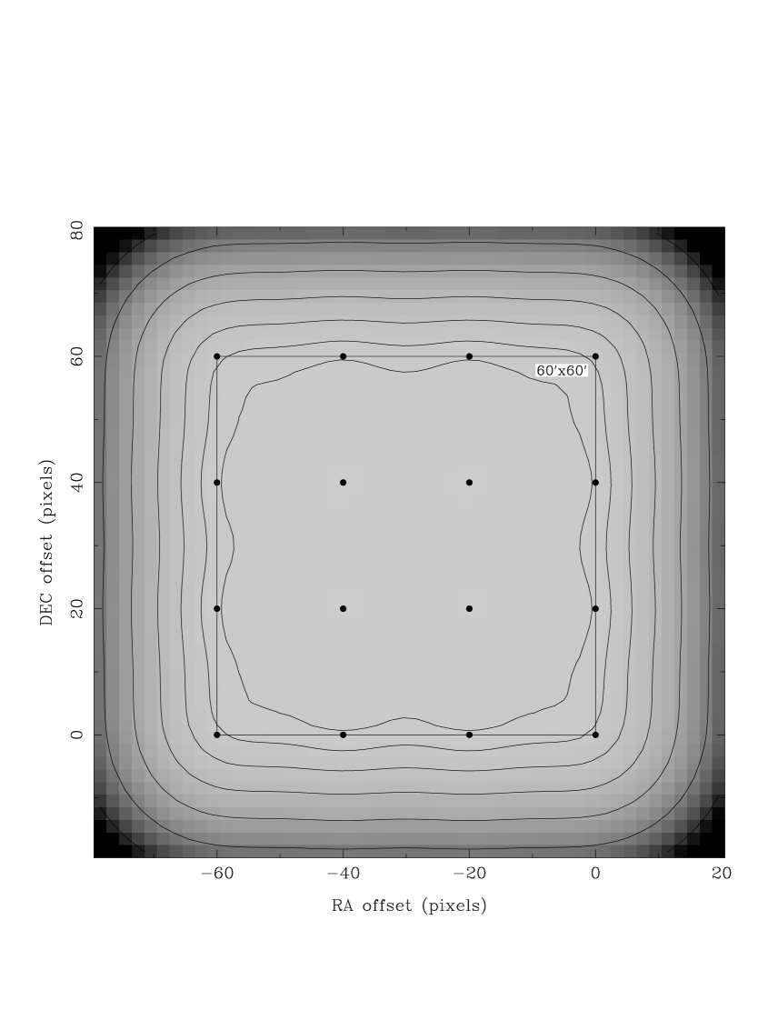
Figure 1: Noise variations expected over a 1 sq.degr. mosaic (central box, 1 pixel $=1\arcmin$) for a $20\arcmin$ spacing rectangular grid. Filled circles indicate the pointing centres. At the center of the mosaic $\sigma(I)/\sigma\sim 1$. Contours refer to 5, 10, 20, 40, 80, 160, 320% noise increment from the center.

2.2 Observing Frequency, Resolution and Sensitivity

At 20 cm (the longest observing wavelength available at the ATCA) the field of view is largest (gaussian primary beam FWHP$\simeq 33\arcmin$) and the system noise is lowest. Thus, observing at 20 cm allows minimization of both the number of fields (i.e. pointings) required to complete the survey and the observing time spent on each field. The ATCA can observe at two frequencies simultaneously (for instance 20 and 13 cm). However, we decided to optimize sensitivity at the expense of spectral information, by setting both receivers in the 20 cm band and observing in continuum mode ($2\times 128$ MHz bandwidth, each divided into $32\times 4$ MHz channels in order to reduce the bandwidth smearing effect). This choice was also influenced by another consideration: since the field of view depends on the observing frequency, the grid pattern could not be optimized to get uniform sensitivity for both 13 and 20 cm bands simultaneously.
The observations were carried out at full resolution (ATCA 6 km configuration), since the identification follow up benefits from high spatial resolution, and the expected fraction of very extended sources (that could be resolved out and lost) is low at the ATESP resolution. Using the angular size distribution given by Windhorst et al. (1990) for radio sources, we estimate that $\ga 70\%$ of the mJy and sub–mJy sources would appear point–like at the ATESP resolution, and $\la 5\%$ would have angular sizes twice the beam size or larger.
Since the ESP sample distance distribution peaks at $z\simeq 0.1$ and ‘normal’ galaxies are typically low-power radio sources, deep radio observations were needed to ensure detections of a statistically significant number of ESP galaxies. We considered satisfactory a point source radio limit of the order of $\sim 0.2$ mJy ($3\sigma$), which corresponds to a detection threshold of $P\sim 3\times 10^{21}$ W Hz^-1 at $z\sim 0.1$ (H${}_{\rm o}=100$ km/s Mpc^-1). Furthermore a large sample of sub-mJy radio sources can be constructed at a $6\sigma$ detection limit, corresponding to a flux limit of $\sim 0.5$ mJy.

3 Observations and calibration

To cover the two areas of $22\degr\times 1\degr$ (region A) and $5\degr\times 1\degr$ (region B) of the ESP survey with uniform sensitivity, $69\times 4$ and $15\times 4$ pointings at $20\arcmin$ spacing are needed respectively. An area of 1.3 sq. degs. ($4\times 4$ pointings) of region A was not observed, because of the presence of the strong radio source PMNJ2326-4027, which would have prevented us from reaching the deep noise level required. This reduced the total number of fields to be observed to $65\times 4$ (region A) and $15\times 4$ (region B), i.e. $320$ pointings in total. The right ascension range actually covered by the ATESP survey is thus $23^{\mathrm{h}}31^{\mathrm{m}}$ – $01^{\mathrm{h}}23^{\mathrm{m}}$ and $22^{\mathrm{h}}32^{\mathrm{m}}$ to $22^{\mathrm{h}}57^{\mathrm{m}}$ (J2000).
An observing time of 1.2 hours per pointing was needed to reach a $3\sigma$ RMS noise level of $\simeq 0.2$ mJy (with $2\times 128$ MHz bandwidth). To obtain good hour angle coverage we organized the snapshot observations as follows: the 320 fields were divided in 16 sets of 20 fields each ($5\times 4$). Every set was then observed for $2\times 12^{\mathrm{h}}$, that is, the 20 fields were observed in sequence, for 1 minute each, repeating this for 72 times and adding 3 minutes for calibration every hour.
The observing campaign started in November 1994 and was completed in January 1996. A log of the observations is given in Table 2 (dates, arrays used, observing time and frequencies). We stress that, for our purposes, the use of different 6 km arrays is not relevant in any way.
The two 128 MHz observing bands were set in the most interference-free region of the 20 cm band (1.3–1.5 GHz).
The flux density calibration was performed through observations of the source PKS B1934-638, which is the standard primary calibrator for ATCA observations ($S=14.9$ Jy at $\nu=1384$ MHz, Baars et al. Baarsetal77 (1977) flux scale). The phase and gain calibration was based on observations of secondary calibrators, selected from the ATCA calibrator list. Every single $12^{\mathrm{h}}$ run and each of the two observing bands were calibrated separately following the standard procedures for ATCA observations.

Table 2: Log of the observations.

Date	$t_{\mathrm{obs}}$	Array	$\nu_{1}$	$\nu_{2}$
	$h$		MHz	MHz
18/11/94–21/11/94	$3\times 12$	6D	1344	1452
23/12/94–04/01/95	$13\times 12$	6A	1344	1452
15/12/95–01/01/96	$17\times 12$	6C	1344	1448

4 Data reduction

For the data reduction we used the Australia Telescope National Facility (ATNF) release of the Multichannel Image Reconstruction, Image Analysis and Display (MIRIAD) software package (Sault et al. Setal95 (1995)). A number of steps in the reduction process are usually done interactively, specifically the removal of bad data (‘flagging’), and, in a certain measure, cleaning and self calibration. Due to the large amount of data involved we found it more practical to develop a semi-automated reduction pipeline.

4.1 Flagging of bad data

Table 3: Main parameters for the 16 final mosaics.

Mosaica	Fields	Tangent Pointb		Synthesized Beamc		$S_{\mathrm{min}}$	$\sigma_{\mathrm{fit}}$	$<\sigma>$
fld $x$ to $y$	$n\times m$	$\alpha_{0}$	$\delta_{0}$	$b_{\mathrm{min}}\times b_{\mathrm{maj}}$	P.A.	mJy	$\mu$Jy	$\mu$Jy
fld01to06	$6\times 4$	22 35 57.37	-39 59 15.0	$7.8\arcsec\times 12.9\arcsec$	$1\degr$	$-0.49$	78.7	$78.5\pm 3.0$
fld05to11	$7\times 4$	22 44 57.60	-39 59 15.0	$7.8\arcsec\times 12.8\arcsec$	$3\degr$	$-0.96$	77.8	$78.5\pm 3.8$
fld10to15	$6\times 4$	22 53 21.68	-39 59 15.0	$7.9\arcsec\times 13.0\arcsec$	$-1\degr$	$-0.70$	88.1	$84.1\pm 5.3$
fld20to25	$6\times 4$	23 34 56.09	-39 58 48.0	$8.5\arcsec\times 16.8\arcsec$	$1\degr$	$-0.68$	83.0	$80.3\pm 4.3$
fld24to30	$7\times 4$	23 43 38.26	-39 58 48.0	$9.5\arcsec\times 16.6\arcsec$	$-2\degr$	$-0.50$	82.8	$83.2\pm 6.4$
fld29to35	$7\times 4$	23 52 20.43	-39 58 48.0	$8.9\arcsec\times 16.7\arcsec$	$2\degr$	$-0.53$	79.2	$76.2\pm 2.9$
fld34to40	$7\times 4$	00 01 02.59	-39 58 48.0	$8.0\arcsec\times 14.5\arcsec$	$5\degr$	$-0.48$	76.3	$74.8\pm 4.0$
fld39to45	$7\times 4$	00 09 44.76	-39 58 48.0	$8.6\arcsec\times 14.3\arcsec$	$-10\degr$	$-0.61$	81.2	$80.4\pm 3.4$
fld44to50	$7\times 4$	00 18 26.93	-39 58 48.0	$7.4\arcsec\times 14.0\arcsec$	$7\degr$	$-0.43$	78.0	$76.4\pm 1.7$
fld49to55	$7\times 4$	00 27 09.10	-39 58 48.0	$8.0\arcsec\times 12.9\arcsec$	$10\degr$	$-0.62$	78.6	$77.1\pm 1.4$
fld54to60	$7\times 4$	00 35 51.26	-39 58 48.0	$8.2\arcsec\times 12.6\arcsec$	$4\degr$	$-0.42$	77.3	$75.8\pm 1.3$
fld59to65	$7\times 4$	00 44 33.42	-39 58 48.0	$7.7\arcsec\times 12.5\arcsec$	$4\degr$	$-0.44$	79.4	$77.8\pm 1.4$
fld64to70	$7\times 4$	00 53 15.58	-39 58 48.0	$7.7\arcsec\times 12.6\arcsec$	$1\degr$	$-0.45$	75.1	$74.6\pm 2.2$
fld69to75d	$7\times 4$	01 01 57.70	-39 58 48.0	$7.5\arcsec\times 12.8\arcsec$	$-2\degr$	$-0.47$	81.9	$79.3\pm 2.1$
fld74to80	$7\times 4$	01 10 39.86	-39 58 48.0	$7.0\arcsec\times 15.0\arcsec$	$1\degr$	$-0.61$	77.1	$76.3\pm 3.8$
fld79to84	$6\times 4$	01 19 22.03	-39 58 48.0	$6.8\arcsec\times 14.3\arcsec$	$7\degr$	$-0.41$	68.9	$67.6\pm 3.5$
a $x$ and $y$ refer to the first and last field columns composing the mosaic. b J2000 reference frame.
c P.A. is defined from North through East. d Reported values for $S_{\mathrm{min}}$ and noise refer to masked mosaic (see text).

We made a modified version of the MIRIAD task TVFLAG (inserted in MIRIAD as TVCLIP), which recursively flags visibilities with amplitudes exceeding a given threshold. The threshold was set as a convenient multiple of the average absolute deviation ($|\Delta S|$) from the running median, evaluated separately for each baseline, each channel and each integration cycle (10 s).
For the primary calibrator the automated flagging procedure was applied before the calibration. This was necessary to avoid the calibration being affected by bad data. For the secondary calibrators and the mosaic data the bandpass and instrumental polarization calibration were applied before running TVCLIP. As we noticed that the shortest baselines introduced some low level, spatially correlated features in the images, which could affect the zero level for faint sources, we decided to remove all baselines shorter than 500 m from the data prior to the pipeline processing (rejection of $\sim 10\%$ of the visibilities). As a consequence, the ATESP survey becomes progressively insensitive to sources larger than $30\arcsec$: assuming a Gaussian shape, only $50\%$ of the flux for a $30\arcsec$ large source would appear in the ATESP images. However, the expected fraction of sources with angular sizes $\geq 30\arcsec$ is very small: $\leq 2\%$ at fluxes $S\leq 1$ mJy according to the Windhorst et al. (1990) angular size distribution.

4.2 Cleaning and Self-calibration

Since the primary beam response is frequency dependent, we did not merge the data from the two observing bands before imaging and cleaning. This results in a slightly poorer UV coverage but allows the cleaning process to succeed in subtracting correctly 100% of the source flux, and self-calibration to be more effective and reliable.
On the other hand, to improve UV coverage and sensitivity, for each field we have merged the (calibrated) data coming from all the observing runs.
In contrast with the imaging of extended sources, joint deconvolution is not needed for a point source survey. It is also very expensive computationally for high resolution images. We therefore reduced every field separately, simplifying imaging considerably.
For each field a $2048\times 2048$ pixel image (total emission only) was produced (pixel size = $2.5\arcsec$). The entire image was then cleaned in order to deconvolve all the sources in the field. To improve sensitivity we used natural weighting, which gave a synthesized beam typically of the order of $8\arcsec\times 14\arcsec$.
Each image went through different cleaning cycles. First, we produced the list of the brightest components to use as model for self-calibration. Phase only self-calibration was applied. Usually two iterations were sufficient to remove phase error ‘stripes’ and improve the image quality.
The self-calibrated visibilities were then used to produce a deeper cleaned image. A serious problem arises if snapshot images are cleaned too deeply. Due to the incomplete UV coverage the number of CLEAN components can approach the number of independent UV points. At this point the cleaning algorithm is not well constrained anymore and can interprete noise (sidelobes, calibration errors, etc.) as CLEAN components. This process can redistribute the noise into the sources and, as a result, the process does not converge and, in principle, the image can be cleaned to zero flux. This produces many faint spurious sources, while the flux of real sources is systematically underestimated. This effect has been mentioned by Condon et al. (Condon98 (1998)) and White et al. (White97 (1997)) for deep snapshot observations with the VLA and is referred to as ‘clean bias’.
From our tests we found that cleaning down to $3\sigma$, the noise gets $\sim 20\%$ lower than theoretical. Down to $2\sigma$ it is a factor of two lower and at $1\sigma$ can be 4–5 times lower. Thus we decided to stop any cleaning process when the peak flux residuals are of the order of 4–5 times the theoretical value (setting a cut-off of 0.5 mJy) to minimize the clean bias (a few percent effect expected, but see discussion in Sect. 5.3).
After this first phase of self-calibration and deep cleaning, we subtracted the sources from the visibility data and we repeated the flagging procedure on the residual visibilities in order to reduce the ‘birdies’ effect mentioned in Sect. 5.1 below.
We then proceeded with another phase of cleaning, and produced a half-resolution residual image covering 4 times the original area; only external parts of this image were cleaned (not the inner quarter, corresponding to the original field, which was already cleaned down to 0.5 mJy). This procedure allowed us to remove the sidelobes from more distant sources (belonging to adjacent fields). These new components were subtracted from visibility data before restoring the sources in the final cleaned image.
As a final step we checked for bright, extended sources in the field, which needed deeper cleaning. A small box containing such a source was cleaned, to a $2\sigma$ level. In general, the application of all these cleaning steps produced good quality single field images.

Figure 2: One of the $6\times 4$ fields mosaiced images. The rectangular box indicates the region corresponding to the ESP redshift survey.

4.3 Mosaicing

The cleaned single field images were co-added in mosaics in order to improve the signal to noise ratio and get uniform sensitivity. Each set of $5\times 4$ fields observed in $2\times 12^{\mathrm{h}}$ observing blocks produces a separate independent mosaic; an overlap between adjacent mosaics was created by adding one (or two) extra column(s) of fields to the side(s) of each mosaic.
Before any mosaic is produced, every field was restored using the same values for the beam parameters. The restoring parameters were chosen as the average value of all the fields composing the mosaic at both frequencies.
The final mosaics were obtained in two steps. First a single frequency mosaiced image was produced for each of the two observing bands, then the final mosaic was obtained by averaging (pixel by pixel) the two initial mosaics in order to improve the sensitivity.
One of our final mosaics is shown in Fig. 2 as an example. The rectangular box indicates the region corresponding to the ESP redshift survey, where the radio survey was designed to give uniform noise. Such a region covers an area of $1.67\degr\times 1\degr$ or $2\degr\times 1\degr$ for mosaics composed by $6\times 4$ or $7\times 4$ fields respectively (see Table 3). Hereafter we will always refer to the central box only in our mosaic analysis. All mosaics are available through the ATESP page at http://www.ira.bo.cnr.it.

5 Mosaic analysis

Table 3 summarizes the main parameters for the final 16 mosaics: for each mosaic are listed the number of fields composing it (columns $\times$ rows), the tangent point (sky position used for geometry calculations) and the synthesized beam (size and position angle). The spatial resolution can vary from mosaic to mosaic depending on the particular array (6A, 6C or 6D) used in the observations. The mean value for the synthesized beam is $\sim 8\arcsec\times 14\arcsec$.

Figure 3: Histogram of the (residual) flux in one of the $6\times 4$ fields mosaiced images (fld01to06). As expected the flux is peaked at zero and the distribution is gaussian.

5.1 Noise

The last three columns of Table 3 show the results of the noise analysis. For each mosaic we report the minimum (negative) flux ($S_{\mathrm{min}}$) recorded on the image (typically $|S_{\mathrm{min}}|$ is of the order of $0.5$ mJy, corresponding to the value at which we have stopped the cleaning) and the noise level. This has been evaluated either as the FWHM of the gaussian fit to the flux distribution of the pixels (in the range $\pm S_{\mathrm{min}}$), in order to check for correlated noise ($\sigma_{\mathrm{fit}}$), or as the standard deviation of the average flux in several source-free sub-regions of the mosaics, in order to verify uniformity ($<\sigma>$).
As expected, the noise distribution is fairly uniform within each mosaic and from mosaic to mosaic ($<10\%$ variations). Also, for each mosaic, the two noise values are consistent, that is the noise can be considered gaussian (see also Fig. 3).
On average the noise level is $\sim 79$ $\mu$Jy. The typical detection limits for the ATESP survey are thus $\sim 0.24$ mJy at $3\sigma$ and $\sim 0.47$ mJy at $6\sigma$. Dynamic range problems can cause slightly higher noise levels of $\sim 100$ $\mu$Jy around strong sources ($S_{\mathrm{peak}}>50-100$ mJy). Such problems appear to be serious only in one mosaic (fld69to75): the region around the bright radio source PMNJ0104-3950 suffers from a very high noise level and a number of spurious sources are present. This was due to strong phase instabilities during the observations which could not be removed by self-calibration. This region (of size $\sim 20\arcmin\times 25\arcmin$) was masked and therefore excluded from further analysis. Excluding this region, the total unifom sensitivity area covered by the ATESP survey is $25.9$ sq. degr. or $7.9\;10^{-3}$ sr.

5.2 Artefacts

Another problem we faced was the possible presence of artefacts in the images, like spurious sources (‘ghosts’) at a level of 0.1–0.5% opposite to bright sources with respect to the phase center of the image and ‘holes’ in the centre of the field. The first problem, caused by the Gibbs phenomenon, arises from the use of an XF correlator and can be serious in high dynamic range continuum observations (like ours). The second effect is a system error produced by the harmonics of the 128 MHz sampler clock at 1408 MHz. Both effects can be completely removed as long as the observing bands are centered appropriately (Killeen Killeen95 (1995); Sault Sault95 (1995)). Unfortunately, at the time of our first two observing runs these effects were not yet known. We therefore could apply the corrections only to the data taken in the last observing run.
We point out that the corrections, when applied, result in a larger bandwidth smearing effect, since only $13\times 8(10)$ MHz channels are used (instead of $32\times 4$ MHz).
Wherever not corrected for, the ‘ghosts’ problem is unlikely to be serious in our case, since ‘ghosts’ appear in different places for each field and so they tend to average out when mosaicing the fields. Moreover, only radio sources brighter than $\sim 100$ mJy can produce detectable ‘ghosts’ in the final mosaics and such bright sources are very few in the region surveyed ($\sim 30$) and therefore could be easily checked. No evident ‘ghosts’ have been found.
We have also tried to reduce the sampler clock self-interference effect as far as possible by flagging residual bad visibilities (that is correlated noise) after a first step of cleaning and self-calibration (see also Sect. 4.2), but some of our fields still show it to a small extent. On the other hand the area of sky affected by ‘holes’ is of the order of a few percents ($\la 3\%$) of the total region observed.

5.3 Clean Bias

Table 4: clean bias average corrections (see text).

Mosaic	cc’s	$a$	$b$
fld34to40	$1616$	$0.09\pm 0.04$	$0.85\pm 0.08$
fld44to50	$2377$	$0.13\pm 0.03$	$0.75\pm 0.06$
fld69to75	$3119$	$0.16\pm 0.05$	$0.67\pm 0.09$

Figure 4: The source flux measured after the cleaning ($S_{\mathrm{output}}$) normalized to the true source flux ($S_{\mathrm{input}}$) as a function of the flux itself (expressed in terms of $\sigma$) is shown for three different cases: 1616 cc’s mosaic (top panel), 2377 cc’s mosaic (middle panel) and 3119 cc’s mosaic (bottom panel). Also shown are the linear fits (see text).

Figure 5: We present $S_{\mathrm{output}}/S_{\mathrm{input}}$ as a function of the average number of clean components. Each dotted line refers to a different source flux ($100\sigma$, $50\sigma$, $30\sigma$, etc.). Also shown is the average number of clean components for each of our 16 mosaics (full lines at the bottom of the figure).

As already mentioned in Sect. 4.2, when the UV coverage is incomplete, the cleaning process can ‘steal’ flux from real sources and redistribute it on top of noise peaks producing spurious ones.
To quantify the actual effect in our mosaics we performed a set of simulations by injecting point sources in the survey UV data at random positions. Then the whole cleaning process was started. The number of sources injected in a mosaic ($\sim 500$) was chosen in order to reduce the statistical uncertainty without changing significantly the components/image statistics. The source fluxes cover the entire range of the survey: 250 sources at 3$\sigma$, 100 at $5\sigma$, 50 at $7\sigma$, 50 at $10\sigma$, 25 at $20\sigma$, 10 at $30\sigma$, 10 at $50\sigma$, 10 at $100\sigma$.
Taking into account the time and frequency resolution and the baseline lenghts, we get about 1500–2500 indepentent UV points for each field observed. This means that with about 2000 independent (not too close together or on top of each other) clean components we could clean the image to zero flux. The average number of (not independent) clean components per mosaic ranges between 1500 and 3200. Since we used a clean loop gain factor $g=0.1$, the number of independent clean components per mosaic can be estimated as 1/10 of the numbers reported above. We thus expect a significant clean bias effect (10-20%), larger for mosaics with a higher number of cleaning components. We then decided to test three mosaics, with a low, an intermediate and a high average number of cleaning components (cc’s) respectively: fld$34$to$40$ (1616 cc’s), fld$44$to$50$ (2377 cc’s) and fld$69$to$75$ (3119 cc’s).
The results of the tests are presented in Fig. 4 and Fig. 5 and summarized in Table 4. Fig. 4 shows, for each of the three mosaics, the average source flux measured after the cleaning ($S_{\mathrm{output}}$) normalized to the true source flux ($S_{\mathrm{input}}$) as a function of the flux itself (expressed in terms of $\sigma$). In general the clean bias increases going to fainter fluxes and, as expected, depends on the number of cleaning components. In the best case (1616 cc’s) we get $\leq 10\%$ flux underestimation for the faintest sources; in the worst case (3119 cc’s) the effect rises up to $\sim 20\%$.
The dependency of the clean bias on the number of cleaning components is more clearly shown in Fig. 5. Here we present $S_{\mathrm{output}}/S_{\mathrm{input}}$ as a function of the average number of clean components for different source fluxes ($100\sigma$, $50\sigma$, $30\sigma$, etc.). Again, the clean bias affects more seriously the faintest sources. Moreover it is evident that we are not dealing with a linear effect: a sudden worsening appears at fluxes of the order of 10–20$\sigma$ and when the number of cleaning components exceeds $\sim 2000$.
A first order fit of the clean bias effect for the three different mosaics has been obtained by applying the least squares method to the function $S_{\mathrm{output}}/S_{\mathrm{input}}=a\log(S_{\mathrm{input}}/\sigma)+b$. The values obtained for the parameters $a$ and $b$ are listed in Table 4 and the curves are shown in Fig. 4.

6 Summary

The ATESP survey at 1.4 GHz is based on snapshot observations of 320 overlapping primary beam fields, reduced separately and then combined together to produce 16 big mosaiced images. The total area surveyed with uniform sensitivity ($1\sigma$ noise level $\sim 79\mu$Jy) covers 25.9 sq. degr. The spatial resolution is typically $\sim 8\arcsec\times 14\arcsec$ providing radio positions with internal accuracy of the order of 1 arcsec for $6\sigma$ radio sources.
We stress the importance of estimating the relevance and the behaviour of the so called clean bias effect for any deep survey obtained with snapshot observations. The source fluxes can be seriously affected by such problem and for reliable scientific analysis the effect must be taken into account and corrected for.

Future papers in this series will deal with:

1. the radio sources catalogue complete down to a limiting $6\sigma$ flux density of $\sim 0.5$ mJy

2. the ATESP radio source counts

3. the radio properties of the ESP galaxies and the local bivariate luminosity function

4. the optical identifications and spectroscopy of the objects in the EIS sub-region.

- (1) Baars J.W.M., Genzel R., Pauliny-Toth I.I.K., Witzel A., 1977, A&AS 61, 99
- (2) Ciliegi P., McMahon R.G., Miley G., et al., 1999, MNRAS 302, 222
- (3) Condon J.J., 1984, ApJ 287, 461.
- (4) Condon J.J., 1989, ApJ 338, 13.
- (5) Condon, J.J., 1996. In Ekers R.D., Fanti C., and Padrielli L. (eds.) Proc. IAU Symp. 175, Extragalactic Radio Sources. Kluver, Dordrecht, p. 535
- (6) Condon J.J., Mitchell K.J., 1984, AJ 89, 610
- (7) Condon J.J., Cotton W.D., Greiser E.W., et al., 1998, AJ 115, 1693
- (8) de Ruiter H.R., Zamorani G., Parma P., et al., 1997, A&AS 319, 7
- (9) Hopkins A.M., Mobasher B., Cram L., Rowan-Robinson M., 1998, MNRAS 296, 839
- (10) Gruppioni C., Zamorani G., de Ruiter H.R., et al., 1997, MNRAS 286, 470
- (11) Gruppioni C., Mignoli M., Zamorani G., 1999a, MNRAS 304, 199
- (12) Gruppioni C., Ciliegi P., Rowan-Robinson M., et al., 1999b, MNRAS 305, 297
- (13) Killeen N., 1995, ATCA Data Acquisition Problems and Information Reports, n. 17
- (14) Kollgaard R.I., Brinkmann W., Chester M.M., et al., 1994, ApJS 93, 145
- (15) Longair M.S., 1966, MNRAS 133, 421
- (16) Mitchell K.J., Condon J.J., 1985, AJ 90, 1957
- (17) Nonino M., Bertin E., da Costa L., et al., 1999, A&AS 137, 51
- (18) Oort M.J.A., 1987, PhD Thesis, Univ. Leiden
- (19) Richards E.A. 2000, ApJ 533, 611
- (20) Richards E.A., Fomalont E.B., Kellermann K.I., et al., 1999, ApJ 526, L73
- (21) Rowan-Robinson M., Benn C.R., Lawrence A., McMahon R.G., Broadhurst T.J., 1993, MNRAS 263, 123
- (22) Sault R.J., 1995, ATCA Data Acquisition Problems and Information Reports, n. 18
- (23) Sault R.J., Killeen N., 1995, Miriad Users Guide.
- (24) Sault R.J., Teuben P.J., Wright M.C.H., 1995. In Shaw R., Payne H.E., Hayes J.E.E. (eds.) Astronomical Data Analysis Software and Systems IV. ASP Conf. Ser. 77, 433
- (25) Vettolani G., Zucca E., Zamorani G., et al., 1997, A&A 325, 954
- (26) Vettolani G., Zucca E., Merighi R., et al., 1998, A&AS 130, 323
- (27) Wall J., Benn G., Grueff G., Vigotti M., 1986. In: Swings (ed.) Highlights of Astronomy. Reidel, Dordrecht, 7, 345
- (28) White R.L., Becker R.H., Helfand D.J., Gregg M.D., 1997, ApJ 475, 479
- (29) Wieringa M.H., Kesteven M.J., 1992, Measurements of the ATCA Primary Beam, ATCA Technical Document Series 39.2010
- (30) Windhorst R.A., van Heerde G.M., Katgert P., 1984, A&AS 58, 1
- (31) Windhorst R.A., Mathis D., Neuschaefer L., 1990. In: Kron R.G. (ed.) Evolution of the Universe of Galaxies. ASP Conf. Ser. 10, 389