The Galactic disk: study of four low latitude Galactic Fields

Abstract

We present deep V and I photometry of stellar field in four previously unstudied low latitude regions of the Galactic disk. All observed fields are located at the western side of the Galactic Center in the direction of the Coalsack-Carina region. They are chosen on the large scale surface photometry of the Milky Way (Hoffmann et al., 1998 and Kimeswenger et al., 1993) and corresponding term maps (Schlosser et al., 1995) as being affected by low interstellar absorption and having integrated colours typical of a very young population. Two of them are suspected to cross the inner spiral arm. More than $10^{5}$ stars are detected in total, down to a magnitude of V $\sim 23.5$. The observational colour-magnitude diagrams (CMDs) and luminosity functions are analyzed using a revised version of the Padova software described in Bertelli et al (1995). The interstellar extinction along the line of sight is derived and found to be in reasonable agreement with Mendez & van Altena (1998) maps. Due to the low galactic latitude of the studied fields, the scale length and mainly the scale height of the thick disk are not strongly constrained by the observations. However a thin disk scale height of about 250$\pm 60$ pc seems to be favored. The data are very sensitive to the star formation rate of the thin disk. A decreasing star formation rate is necessary to reproduce the distribution of the stars in the colour-magnitude diagrams as well as the luminosity functions. A constant or a strongly increasing star formation rate as derived using Hipparcos data for the solar neighborhood (Bertelli et al 1999) are marginally in agreement with the luminosity functions but they are at odds with the CMDs. The analysis of these data suggest that the solar neighborhood star formation rate cannot be considered as representative for the whole thin disk. To properly reproduce the luminosity functions a thick disk component having a local density of about 2–4% must be included. From the star-counts the local neighborhood mass density in stars more massive than 0.1 M_⊙ is found to be 0.036–0.02 M_⊙ pc ^-3. Finally, the location of inner spiral arm is discussed. We find evidence of a population younger than 10⁸ yr distributed in a spiral arm at a distance of 1.3$\pm 0.2$ and 1.5 $\pm 0.2$ Kpc in the directions l$\sim$ 292 and l$\sim$ 305 respectively. This result is consistent with the spiral arm pattern defined on the basis of pulsars and young associations (Taylor & Cordes (1993); Humphreys (1976)). Due to the small field of view two of the studied fields do not set strong constrains on the scale height and lenght of the disk. A larger field of view, see e.g. the WFI at the 2.2m ESO telescope having 30${}^{\prime}\times$ 30^′ would allow us to have good statistics down to faint magnitudes.

1 Introduction

During the past years many efforts have been undertaken to gain information about the structure of the Milky Way. However, several unresolved questions still remain. A program has been recently started to study the structure of the Galaxy by means of deep photometry of stellar populations. Several fields in the direction of the Galactic center has been been analyzed with the aim of studying the Galactic structure; deriving the stellar extinction along the line of sight; obtaining information about the age and the metallicity of the stars in various Galactic components (halo, bulge and disc); deriving the past history of star formation and chemical enrichment.

In brief, Ng et al. (1995) studied the color magnitude diagram (CMD) and luminosity functions (LF) of the field #3 of the Palomar Groningen Survey (PG3) located at the periphery of the Galactic Bulge (l=0, b=-10) and set up the basic tool to deconvolve the contribution from many stellar population to highly composite CMDs. Bertelli et al. (1995) analyzed three regions of the Bulge located near the clusters NGC6603 (l=12.9 b=-2.8 ), Lynga 7 (l=328.8 b=-2.8) and Terzan 1 (l=357.6 b=1.0). First they show that the extinction law greatly varies with the direction towards the center. Second, they trace the position of a molecular ring between 3.5 and 4 kpc in the direction of NGC6603, of a stellar ring between 3.0 and 4.0 kpc, of the Sagittarius arm in the direction of NGC6603 (5.0 to 7.0 kpc) and Lynga 7 (4.2 to 7.0 kpc). Third, they recognize the presence near the Galactic Center of an old and metal rich population (see also the detailed study of the CMD of Terzan 1 by Bertelli et al. 1996 in which evidences for the existence of old, high metallicity stars in the so-called hot horizontal branch stage are found), and finally give a hint that the Galactic Bar points its nearest side toward positive galactic longitude.

This paper is devoted to the study of four low latitude fields in the Galactic disk in the direction of the Coalsack-Carina region. Studying the CMDs and luminosity functions it is possible to determine the age and star formation history of the thin disk components, the extinction along the line of sight derive hints about the scale height and length.

In section 2 and in section 3 the observations and the data reduction respectively are described. In section 4 the CMDs are presented. In section 5 the model and the input parameters are given. In section 6 the results are discussed. The presence of a spiral arm at l$\sim$ 292 and l$\sim$ 305 is analyzed in section 7. Finally, the conclusions are drawn in section 8.

Table 1: General information on the fields: central coordinates, number of exposures and integrated exposure time for both filters, dimension of the selected part of the field (see text for details), and total number of stars therein.

	$\alpha_{2000}$	$\delta_{2000}$	$l$	$b$	$N_{E}(\mbox{V})$	$t_{E}(\mbox{V})/s$	$N_{E}(\mbox{I})$	$t_{E}(\mbox{I})/s$	$size$	$N_{stars}$
Field 1 (F1)	$\,\,\,8^{h}40^{m}54^{s}$	$-46^{\circ}56^{\prime}40^{\prime\prime}$	265.545	$-3.089$	6	1440	6	1080	$6^{\prime}.4\times 9^{\prime}.6$	2787
Field 2 (F2)	$\,\,\,9^{h}38^{m}54^{s}$	$-53^{\circ}13^{\prime}00^{\prime\prime}$	276.448	$-0.546$	10	1800	10	1200	$12{\prime}.0\times 12^{\prime}.0$	6580
Field 3 (F3)	$11^{h}27^{m}33^{s}$	$-59^{\circ}31^{\prime}09^{\prime\prime}$	292.468	$\,\,\,\,1.638$	6	1080	4	720	$9^{\prime}.6\times 9^{\prime}.6$	12153
Field 4 (F4)	$13^{h}13^{m}27^{s}$	$-67^{\circ}39^{\prime}29^{\prime\prime}$	305.029	$-4.876$	5	1500	5	1200	$9^{\prime}.6\times 9^{\prime}.6$	9380

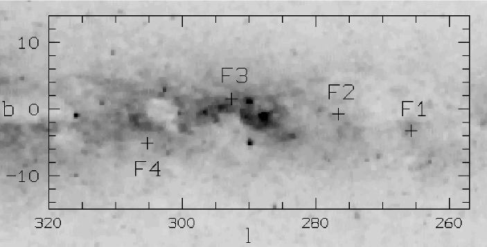
Figure 1: The location of the observed fields are indicated in the Galactic map (V passband) of the Coalsack-Carina region

2 Data

For this work, four fields have been observed in Bessel V and Gunn I with the 1.54 m Danish telescope at the European Southern Observatory (ESO), La Silla (Chile) on February $\rm 10^{th}-13^{th}$, 1997 (camera C1W11/4 with 2k$\times$2k pixels and a nominal field of view of $13^{\prime}\times 13^{\prime}$). The coordinates of the fields, the number of averaged exposures, and the total exposure time per filter are given in Table 1.

The fields have been chosen on the large scale surface photometry maps of the Milky Way (Hoffmann et al., 1998 and Kimeswenger et al., 1993) and corresponding term maps which display all points of the Milky Way having the same colour (Schlosser et al., 1995). These maps show large scale structures and are therefore suitable for the selection of interesting areas. The integrated colours of the fields we select show they are affected by low interstellar absorption. Two of the fields point in the direction of the Sgr–Car arm and their integrated UBVR colors are consistent with the presence of a significantly fraction young population. In Fig. 1, the positions of the observed fields are plotted over the relevant part of the Galactic V map.

3 Reductions

All of the reductions have been carried out with the image processing system MIDAS. For the stellar photometry, the DAOPHOT and ALLSTAR code have been used. The raw data has been corrected for bias and flat-fields. Due to technical problems with the filter wheel resulting in vignetting, the flat-fields are not only very inhomogeneous but do also vary in time. Therefore some of the data couldn’t be used at all. The dimensions of the unvignetted section of each field are given in table 1.

For the calibration, at least 10 standard stars have been measured at the beginning, the middle and the end of every night at different air-masses. They have been selected from Landolt (1992). From the measured standard stars we derive the following relation between instrumental v, (v-i) and calibrated V , (V-I) for 1 sec of exposure time:

$$\begin{array}[]{r@{\;\; = \;\;}l}V-I&1.034\,(v-i)+0.9824\\ V&v+0.007\,(V-I)-1.26\\ \end{array}$$ (1)

The completeness corrections $\Lambda_{V}$ and $\Lambda_{I}$ defined as the ratios of recovered to injected stars in V and I frames respectively are derived by means of the usual artificial stars experiments. They are plotted for each field and filter in Fig. 2. The photometric errors are 0.01,0.05,0.12,0.20 for V=10,21,22,23 respectively and 0.01,0.02,0.05,0.2 for I=10,18,20,21.5 mag.

Figure 2: Completeness factors $\Lambda_{V}$ and $\Lambda_{I}$ as functions of the magnitudes for all the fields.

4 Colour-Magnitude Diagrams (CMDs)

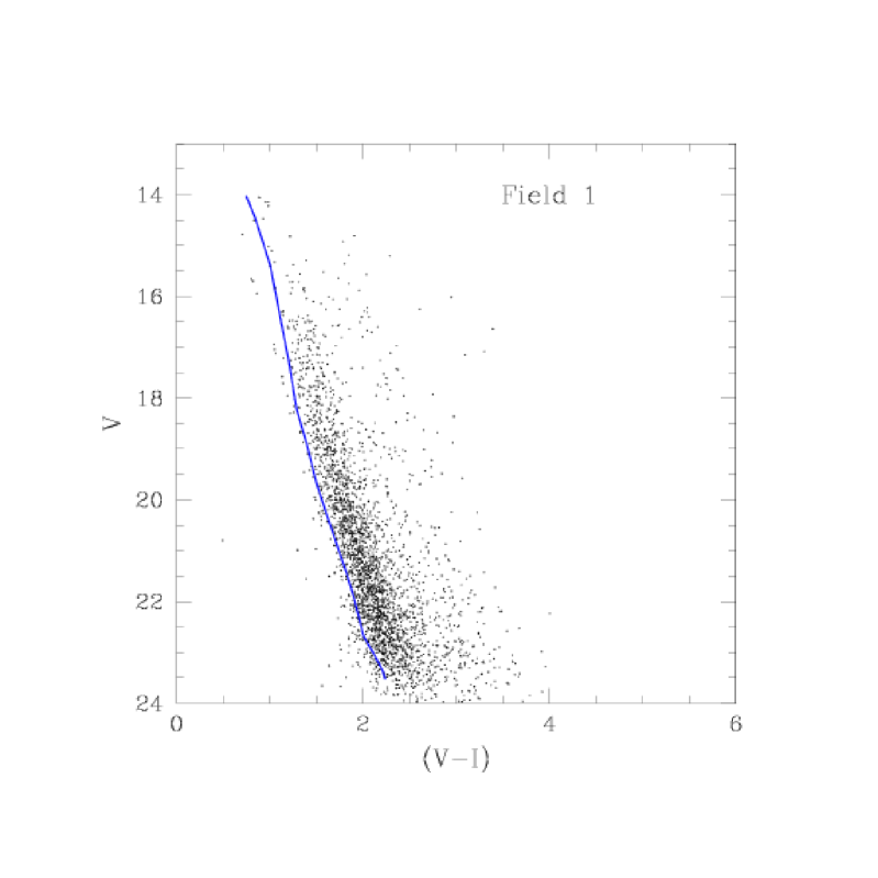
a)

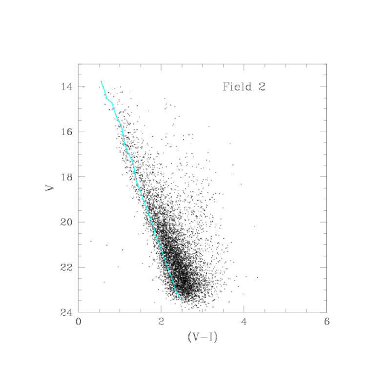
b)

c)

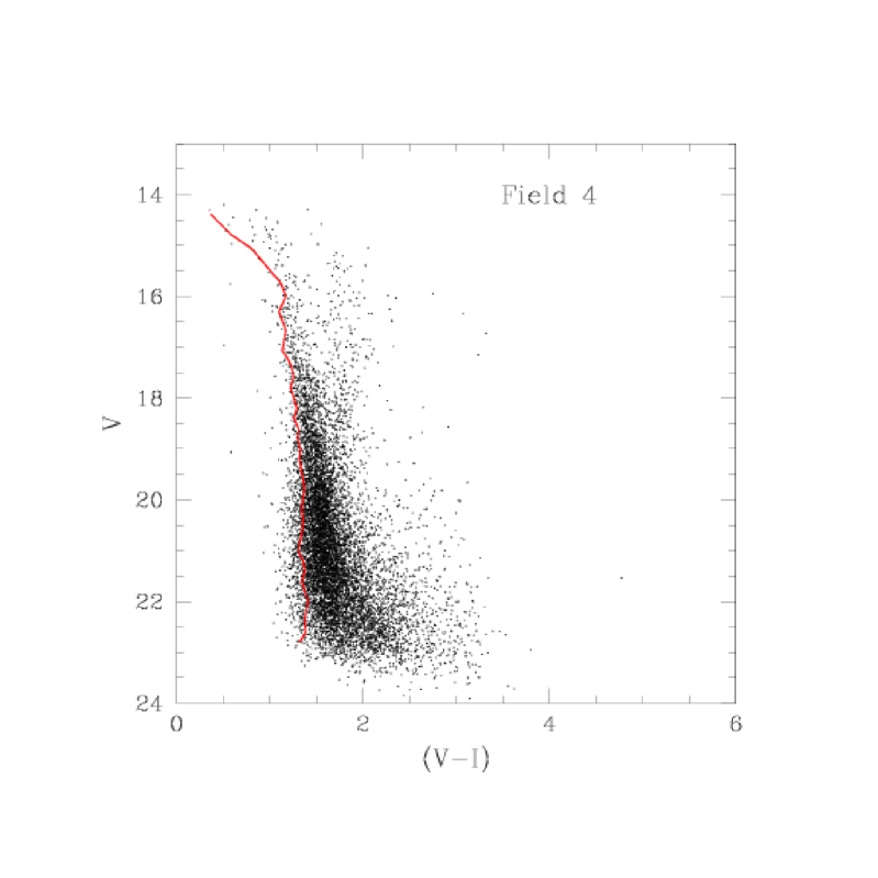
d)

Figure 3: The V–(V-I) CMDs of the fields F1 (a), F2 (b), F3 (c), F4 (d). For all fields, the main sequence population dominates the diagram. The red branch parallel to the main sequence can be identified with evolved stars. The line shows the blue edge of main sequence (see text for details)

In Fig. 3 the resulting V–(V-I)–CMDs are presented for all the fields. In these diagrams the main sequence population is the most prominent feature. In F3 and F4 a red branch parallel to the main sequence is visible. It is produced by He-burning evolved stars distributed along the line of sight with increasing reddening. In the fields F1 and F2 this branch is scarcely populated. The CMDs of F3 and F4 show a small group of stars brighter than V $\sim$ 15–15.5 on the blue side of the main sequence. In section 7, these stars will be shown to be tracers for the inner spiral arm (I).

5 Modeling the Galaxy

The description of the Galaxy is done with the code already described by Bertelli et al. (1995) and revised as described in the following sections. First a synthetic population is generated at varying the parameters age, metallicity range, star formation law and initial mass function. Second, the stars are distributed along the line of side following a model of the Galaxy, where all the components are taken into account. Finally, the photometric completeness of the data is taken into account dividing the simulated CMD in magnitude-colour bins and then subtracting from each bin having N_th stars, (1-$\Lambda$)N_th, where $\Lambda$ is the smallest of the V and I completeness factors given in Fig.2.

The generation of the synthetic population makes use of the set of stellar tracks by Girardi et al. (1996) for Z=0.0001, Bertelli et al. (1990) for Z=0.001, Bressan et al. (1993) for Z=0.020, Fagotto et al. (1994a,b,c) for Z=0.0004, 0.004, 0.008, 0.05, 0.10.

5.1 The star formation rate

The history of the star formation in the solar neighborhood has been derived using various methods. Several authors suggest that a constant star formation rate can be appropriate for the disk (see among the others Twarog 1980, Haywood et al. 1997). On the basis of the Hipparcos data a star formation rate increasing towards younger ages is derived (Bertelli et al 1999). In the following, several star formation rates going from constant to increasing or decreasing in time are adopted and the corresponding CMDs and luminosity functions are compared with the data (see section 6).

5.2 The position of the sun

The position of the sun above the Galactic disk mid-plane is found to range from 10 to 42 pc, the upper limit being obtained by star count method (Stobie & Ishida 1987). On the basis of star-counts in 12 fields in the North and South hemispheres, Humphreys & Larsen (1995) suggest that values as low as 20.5$\pm$3.5 pc are more appropriate. Even lower values of 15$-$14 pc are found by Binney et al. (1997), Haywood et al. (1997), Cohen (1995), Hammersley et al. (1995). However, as pointed out by Haywood et al. (1997) the expected offset of the sun deduced from star-counts is found to depend on the scale height of the disk, in the sense that small scale height value favors small offsets: a scale height of 350 pc is compatible with an offset of 20 pc, while a scale height of 200 pc suggests an offset of 15 pc. In the following we adopt an offset of 15 pc.

The distance of the sun from the Galactic center is discussed from 7 to 8.5 Kpc. We adopt 8 Kpc, as a mean value.

5.3 Thin disk

5.3.1 Mass distribution

Two kind of mass distributions are usually adopted:

1) a double exponential law of the form:

$$$$\rho_{disk}=\rho_{0}e^{-r/h_{r}}e^{(z-z_{\odot})/h_{z}}$$$$ (2)

where $h_{r}$ and $h_{z}$ are the scale length and scale height of the disk, respectively;

2) an exponential distribution on the plane and sech² perpendicularly to the plane:

$$$$\rho_{disk}=\rho_{0}e^{-r/h_{r}}sech^{2}({z-z_{\odot}}/h_{z})$$$$ (3)

For z $>>$ $h_{z}$ the two functions are often considered equivalent. However, in our case, this condition is not always met. In particular, using DIRBE data, Freundenreich (1996) find that the sech² distribution is greatly superior to the exponential at low latitudes ($|b|<5^{\circ}$), as in our case. Both distributions will be considered and discussed. In our formulation, the constant $\rho_{0}$ can be calculated for every model imposing that the total number of stars in a selected region of the observational CMD is reproduced by the simulations. From $\rho_{0}$ the local mass density distribution will be derived (see following sections).

5.3.2 Scale height and scale length

The scale height $h_{z}$ of the thin disk varies from 325 pc (Gilmore & Reid 1983, Reid & Majewski 1993, among others) to 200 pc (Haywood et al. 1997). In our model, this value is assumed as a free parameter.

The scale length $h_{r}$ is found to vary from 3.0 Kpc (Eaton et al. 1984, Freudenreich 1997) to 2.0 Kpc (Jones et al. 1981). Intermediate values are derived by Ruelas-Mayorga (1991), Robin et al. (1992) who give $h_{r}$=2.5 Kpc.

In our description, $h_{r}$ and $h_{z}$ are assumed to be constant with the Galactic radius. This may not be valid in the outer Galaxy, where the dark matter might dominate the mass. In fact radio observations suggest that the thickness of the HI layer reaches about 400 pc at 13 Kpc, while the H2 layer is considerably flatter, reaching 200 pc at 12.5 Kpc of galactocentric distance (see Combes 1991 for a review). However the angle of maximum displacement above the plane is believed to range between 80⁰(Burton 1988) and 110⁰ (Diplas & Savage 1991), measured counterclockwise from the direction l=0. The effect in the fields under discussion is negligible.

5.3.3 The Metallicity

Suggestions have arisen in literature that no age-metallicity relation is present in the thin disk. Edvardson et al. (1993) find a spread of about 0.6 dex in $\Delta[M/H]$ among main sequence stars of similar age in the solar neighborhood: the abundance spread for stars born at roughly the same galactocentric distance is similar in magnitude to the increase in metallicity during the lifetime of the disk. Studies of Galactic open clusters as well as of B stars in the solar neighborhood came to the same conclusion (Friel & Janes 1993, Carraro & Chiosi 1994, Cunha & Lambert 1992). In our simulations, a stochastic age metallicity relation for the disk has been adopted, with Z going from 0.008 to 0.03.

5.3.4 Age components

Up to now the main source of information about the age of this component comes from the open cluster system. If all the open clusters are member of the thin disk, a limiting value might be given by NGC 6791 which is the oldest open cluster with well-determined age. Its age is going from 7 to 10 Gyr (Tripicco et al. 1995). However, Scott et al. (1995) find a somewhat peculiar kinematics for this object. The age of Berkeley 17, which is believed to be one of the oldest disk clusters with 12 Gyr (Phelps 1997) has recently been substantially revised using near-IR photometry to 8-9 Gyr (Carraro et al 1999). A lower limit to the age of the disk is given by the white dwarfs: recent determinations suggest an age of 6-8 Gyr (Ruiz et al. 1996). This value agrees quite well with the oldest age of field population based on Hipparcos data which is 11$\pm 1$ (Jimenez et al 1998). While the youngest age $\tau_{f}$ of the thin disk component is constrained by the CMD, the oldest age is assumed to be 10 Gyr. $\tau_{f}$ turns out to be in the range 1–5 $\times 10^{8}$ yr in all the fields.

The velocity dispersion of the disk stars suggest the presence of more age components, having different scale heights (Bessel & Stringfellow 1993). In the following in addition to the old component with large scale height, a second one is taken into account , having scale height $h_{z1}=100$ pc and ages ranging from $\tau_{B}$ to the final age $\tau_{f}$. $\tau_{B}$ is assumed to be 2 Gyr. This assumption has been verified on the luminosity functions of the observed fields. When $\tau_{B}$ is 3 Gyr, the luminosity functions are difficultly reproduced unless a quite high percentage of thick disk ($>$ 8%) is assumed.

5.4 Thick Disc

5.4.1 The age and the metallicity of the thick disk

The mean metallicity is believed to be compatible with the one of the disk globular clusters (-0.6 to -0.7), even if a metal rich tail is expected up to -0.5 together with a metal poor component down to -1.5 dex (Morrison et al. 1990). Gilmore et al. (1995) find a peak of the iron abundance distribution of F/G thick disk stars at -0.7 dex, with no vertical gradient.

Edvardson et al. (1993) estimate an old age for the thick disk component of the solar neighborhood (about 12 Gyr), with no age gap between the thin-thick disk stars. Gilmore et al. (1995) confirm this result. Since the abundance ratios of the thick disk stars reflect incorporation of iron from type I supernovae, these authors suggest a star formation time scale larger than the time scale of SNI which is about 1 Gyr. The kinematics of the thin and thick disks suggest an evolutionary connection between the two components (Wyse & Gilmore 1992, Twarog & Antony-Twarog 1994). It cannot be ruled out that the thick disk is the chemical precursor of the thin disk and is formed through a dissipational collapse after the halo formation and before the end of the thin disk collapse.

However, other scenarios are presented in literature, suggesting that the thick disk formed after the thin disk, either for secular kinematic diffusion of the thin disk stars, or as the result of a violent thin disk heating due to the accretion of a satellite galaxy (Quinn et al. 1993, Robin et al. 1995). At present, it is quite difficult to discriminate between these two models. In the following, we assume the thick disk has an age range from 12 to 8 Gyr, with constant star formation and a metallicity ranging from Z=0.0006 to 0.008.

5.4.2 The mass distribution

As in the case of the thin disk, two density laws are adopted: either double exponential, or exponential in the plane and following sech(z/z_⊙) perpendicularly to the plane.

The local density of the thick disk population is poorly known, in spite of the attempt made to measure it. From high proper motion stars, Sandage & Fouts (1987), Casertano et al. (1990) find values ranging from 2% to 10% of the total disk density. Large uncertainties are found also from star-counts, since such estimates are correlated with the determination of the scale height. Small local densities are correlated with large scale heights. The values are going from 1% to 10% of the total density. Robin et al. (1995), Haywood et al. (1997) suggest an intermediate value of 5.6% of the local disk population is due to thick disk. In the following we accept only solutions compatible with a thick disk percentage between 2% and 5%.

5.4.3 The scale height and scale length

Reid & Majewski (1993) summarized the results on the scale height of the thick disk. Gilmore (1984) find a scale height of 1300 pc. Norris (1987), Chen (1996), Gilmore & Reid (1983) found values of 1100 pc, 1170 pc, and 1450 pc respectively. Lower values are suggested by Gould et al. (1995) on the basis of HST counts, by Robin et al. (1995), Haywood et al. (1997) using ground based star counts: 760$\pm 50$ pc.

Concerning the scale length of the thick disk Robin et al. (1992), Fux & Martinet (1994), Robin et al. (1995) favor a value of 2.5-2.8 kpc. In our simulations we consider scale height and scale length of the thick disk as free parameters.

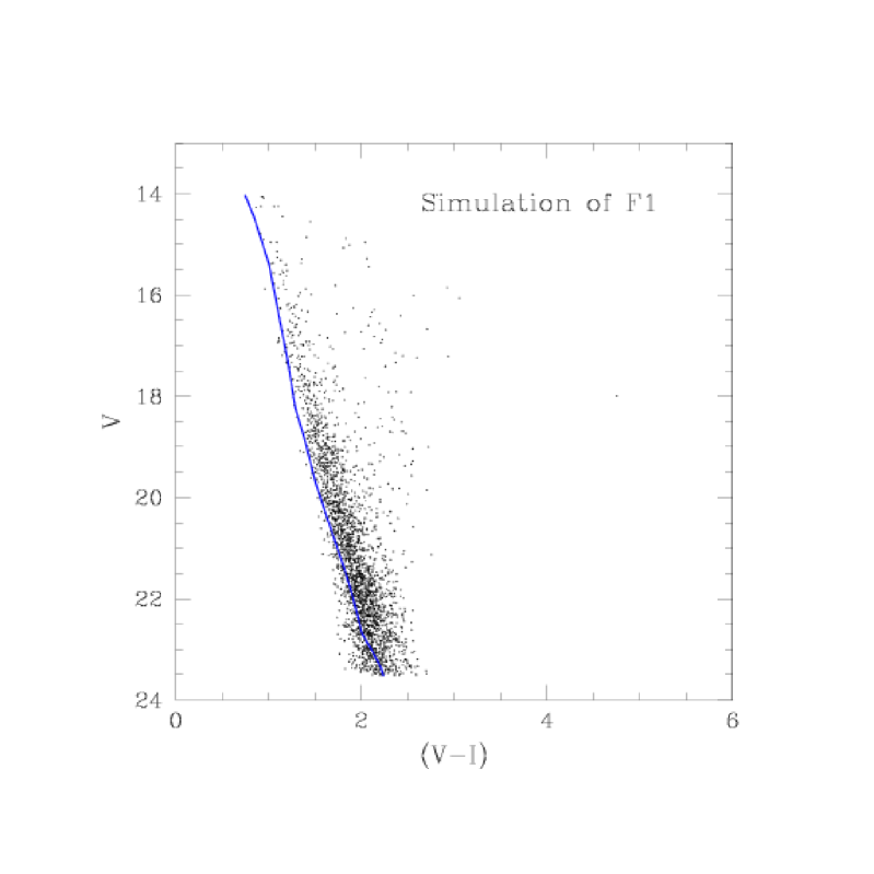
a)

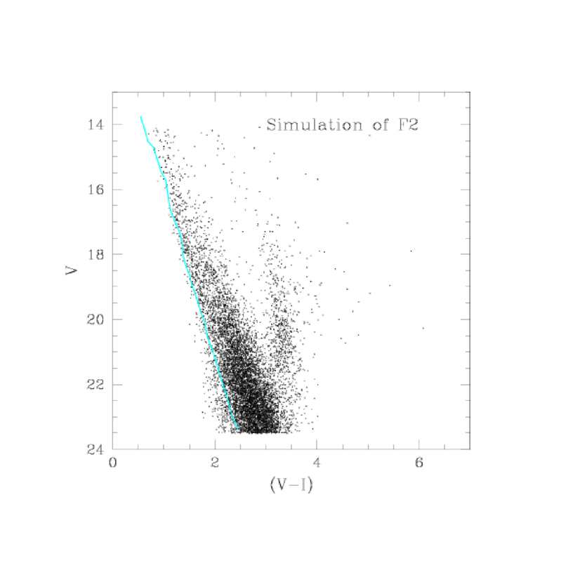
b)

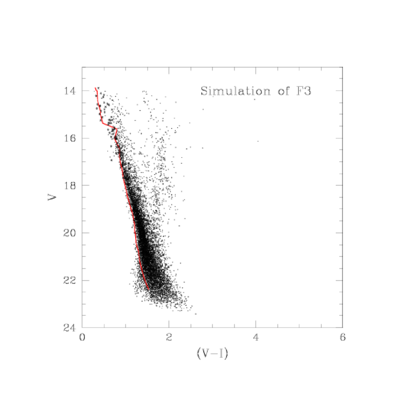
c)

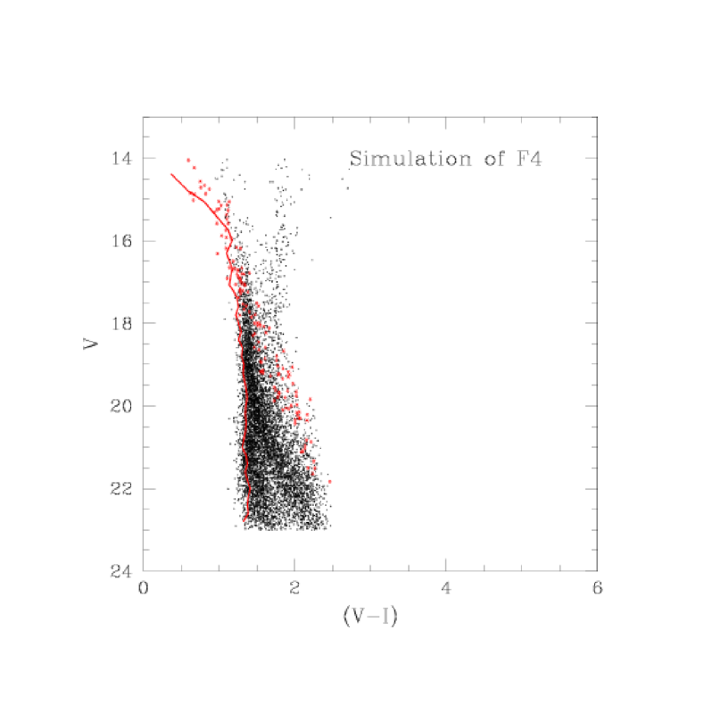
d)

Figure 4: The V–(V-I) CMD of the best solution for each of the fields is shown as example: F1 (a), F2 (b), F3 (c), F4 (d). F1 and F2 simulations include disc components (faint dots), while in the case of F3 and F4 the spiral arm is as well plotted (starred dots). In each plot the line indicates the observational edge of the main sequence. The star formation of the thin disc components is decreasing in time (see text for details).

6 The results

In this Section, the fields will be analyzed separately, deriving the reddening along the line of sight and the possible solutions. For the best fitting solutions the simulated CMDs are displayed in Fig.4. In the simulations of F3 and F4 a young spiral-arm-like population is also included, as described in Section 7. After discussing the single results for each field in the following subsections, they will be compared to derive the best fitting solution for all the fields. Since the studied fields are located at low Galactic latitude, we expect them to be more sensitive to the star formation rate and to the scale height than to the scale lenght of the disk components. For the same reason the parameters of the thick disk component would not be strongly constrained.

6.1 Discussing the CMD: Extinction determinations

Figure 5: The reddening along the line of sight, as determined for the four fields. For comparison, the values of Mendez & van Altena (1998) are included in the plots.

Ng et al. (1995), Bertelli et al. (1995) proved that the slope of the main sequence in the CMD of the disk population is mainly governed by the extinction along the line of sight. At each magnitude $V$ the bluest stars on the main sequence can be interpreted as the envelope of the main sequence turnoffs of the population having absolute magnitude $M_{tur}$, shifted towards fainter magnitudes and redder colours by the increasing distance and corresponding extinction. Starting from an initial guess, the amount of extinction at increasing distances is adjusted until a satisfactory agreement between the main sequence blue edge location in the data and in the theoretical simulations is reached. The comparison between data and simulations is made using a $\chi^{2}$ test. The results are given in Fig. 5.

We point out that F2 and F3 show a relatively modest increase of the interstellar absorption along the line of sight ($\Delta$Ȧ_v less than 0.5 mag) between 1.5 and 2 kpc distance from the Sun for F2 and between 2 and 5 kpc for F3. Whereas this increment in F2 is probably due to some local density increase of the interstellar matter, the increment in F3 can be explained on larger scales since the direction of F3 at l=292 is crossing the inner spiral arm, if the description of the spiral pattern given by Taylor & Cordes (1993) is adopted. At 1.5 Kpc distance from the Sun, the spiral arm is reached (see section 7), at a height of 40 pc above the Galactic plane. At about 5 Kpc distance, the spiral arm is left at a height of 150 pc above the plane. For this field the increase of extinction is well correlated with the intersection of the spiral arm pattern. In Field F4 (l=305) which does also point towards the inner arm, no special increment of the extinction is noticeable. This is not entirely surprising, since the the fields are chosen on the basis of their integrated colours as having low total absorption (see Section 2).

Finally, we would like to address the question whether the trends in the extinction versus the distance shown in Fig. 5 are real. It is quite difficult to give an estimate of the uncertainty on these determinations. However, the simulations show that by changing the extinction of $\pm 0.2$ mag at a given distance d a significant shift in the location of the main sequence edge at magnitudes fainter than $M_{tur}-5+5\times logd+A_{V}$ is produced. We can safely assume that the $A_{V}$ determination of Fig. 5 cannot have an internal error larger than 0.2 mag.

We point out that these determinations of extinction are dependent on the adopted age and metallicity range of the population. To estimate the uncertainty due to the combined effect of different age and metallicity distributions, we derive the extinction separately for the three disk components, namely the young thin, the old thin and the thick disk described in Section . The determination of the extinction along the line of sight $A_{V}$ turns out to be different from the adopted values at maximum of 0.2. To further check these results, we make a comparison with the values derived from reddening maps by Mendez & van Altena (1998). Taking into account the errors on Mendez & van Altena determinations (0.23 mag in E_(B-V), with A_v= 3.2 E_(B-V)) , the agreement is reasonable up to distances of about 8 Kpc, at (l,b)=(292.4,1.63) (field F3), and (305.0,-4.87) (field F4). At (l,b)=(265.54, -3.08) (field F1) and (276.4,-0.54) (field F2) our and Mendez & van Altena (1998) A_v determinations are consistent up to 3–4 Kpc, our values being higher of a factor $\sim 2$ at larger distances.

When the maximum reddening in each direction is compared with the maps by Schlegel et al. (1998) derived using DIRBE data, the agreement is excellent, in spite of the fact the authors claim their values should not be trusted for $|b|<5^{\circ}$.

6.2 Discussing the CMD: the star formation rate

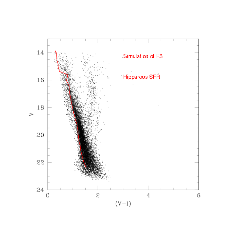
a)

b)

Figure 6: Simulation of the CMD of F3 obtained using the Hipparcos parameterized SFR as described in the text (a). The line shows the observational edge of the main sequence. For sake of easy comparison the observational CMD of F3 (see Fig 3) is as well shown (b).

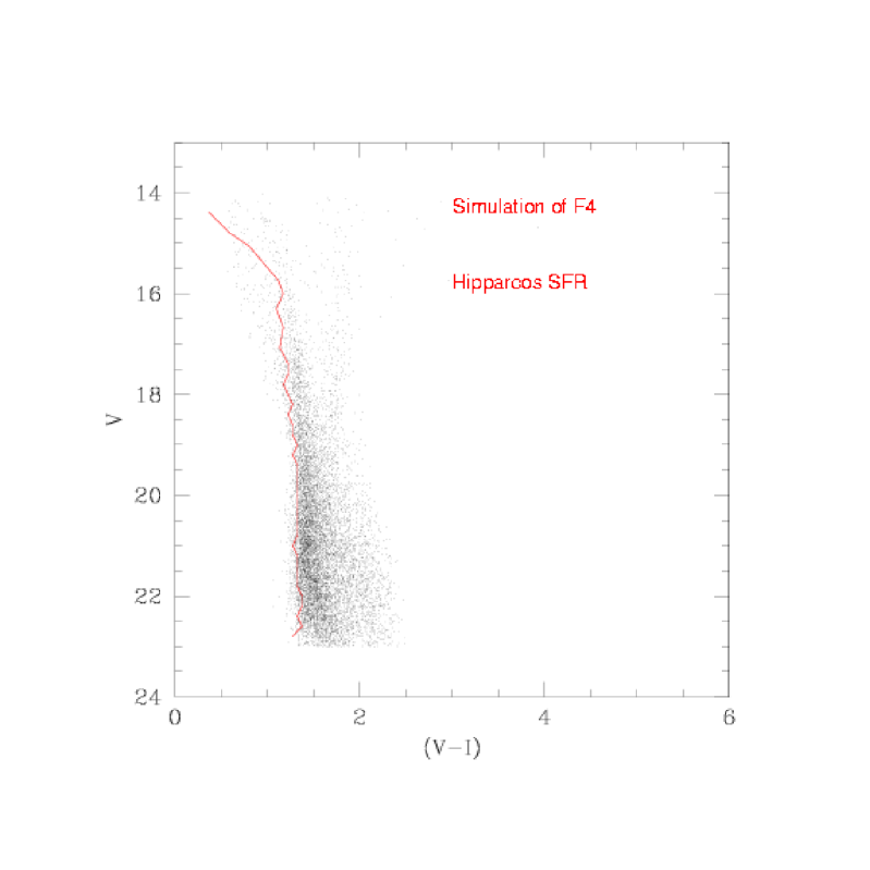
a)

b)

Figure 7: Simulation of the CMD of F4 obtained using the Hipparcos parameterized SFR as described in the text (a). The line shows the observational edge of the main sequence. For sake of easy comparison the observational CMD of F4 (see Fig 3) is as well shown (b).

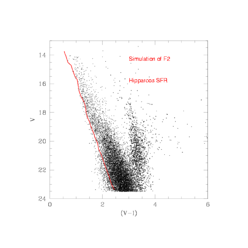
a)

b)

Figure 8: Simulation of the CMD of F2 obtained using the Hipparcos SFR as described in the text. The line shows the observational edge of the main sequence. To allow a easy comparison, the observational CMD of F2 (see Fig 3) is as well shown (b).

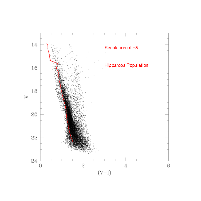
a)

b)

Figure 9: Simulation of the CMD of F3 obtained using the Hipparcos population as described in the text. The line shows the observational edge of the main sequence. For comparison the observational CMD of F3 (see Fig 3) is shown (b).

To infer the star formation rate (SFR) of the thin disk component, simulated CMD and LF are calculated with constant, increasing or decreasing rate and then compared with observational CMDs using a $\chi^{2}$ test. The thick disc is assumed to have a SFR constant from 11 Gyr to 8 Gyr. Due to the low galactic latitude of the observed fields, it is not possible to distinguish between constant or slightly increasing/decreasing rate for this component.

From the analysis of the Hipparcos data Bertelli et al. (1999) derive a disk SFR constant from 10 Gyr to 4.5 Gyr, and then increasing by a factor of 1.5-2 from 4.5 Gyr to 0.1 Gyr. However it is not straightforward that the SFR found in the solar neighborhood is representative of the whole disk, as has already been suggested by Bertelli et al. (1999).

To assess this point, we simulate the CMDs and luminosity functions of the fields using the parameterization of the SFR derived from the Hipparcos data by Bertelli et al. (1999). While the luminosity functions are not inconsistent with this SFR, the CMDs of F3 and F4 cannot be reproduced, since too many young stars brighter than V=19.5 and bluer than the main sequence observational edge are produced. This is evident comparing the simulated and the observed CMDs of F3 and F4 in Fig. 6 and Fig.7. The extinction cannot be responsible of this discrepancy: if the extinction along the line of sight at closer distances is increased to match the observational location of the blue edge of the main sequence at brighter magnitudes, then the faint main sequence turns out to be too red.

The case of F1 and F2 is substantially different. In these fields the blue edge of the main sequence is reproduced using the Hipparcos SFR (see Fig. 8 for F2). However, too many evolved stars are expected in F2 (740 stars brighter than V=22) in comparison with the data (80 stars). No additional information is coming from F1. Due to the poor statistic, the observed and the expected number of stars in this field (63 and 74 respectively) are compatible inside the errors.

However, it cannot be excluded that this result is dependent on the adopted parameterization of the solar neighborhood star formation. To make a further check we use the observed Hipparcos population, and we distribute it along the line of sight in the disk. The resulting CMD is presented in Fig. 9 for F3. The previous conclusions are substantially unchanged. Similar result can be reached in the case of F4, not shown for conciseness.

From this investigation we conclude that the solar neighborhood cannot be considered representative of the properties of the whole disk. An analogous discussion can be made at varying SFR. The simulations show that any assumption of an increasing or even constant SFR yields a too high number of young stars on the blue side of the main sequence. Actually, the most convincing result is obtained with a SFR constant from 10 Gyr to 2 Gyr, then declining by a factor of 10 between 2 Gyr and 0.1 Gyr (see Fig.4).

As a final comment, the CMDs of F3 and F4 show an additional sprinkle of stars brighter that V $\sim$ 15.5 mag and bluer than the mean location of the main sequence (see Fig. 3). These stars cannot be reproduced unless a young burst of star formation well confined in distance is assumed. This feature will be proved to be consistent with the presence of a spiral arm (see section 7).

6.3 The results for F3

Figure 10: The luminosity function of F3 is displayed with the four selected solutions. Solutions a),b),c) are calculated using a sech² mass distribution, solution d) is making use of the exponential mass distribution:
a) $\rm h_{r}=2.5\,kpc$, h${}_{z}\rm(thin)$=0.22 kpc, h${}_{z}\rm(thick)$= 1.0 kpc;
b) $\rm h_{r}=3.0\,kpc$, h${}_{z}\rm(thin)$=0.21 kpc, h${}_{z}\rm(thick)$= 1.5 kpc;
c) $\rm h_{r}=3.0\,kpc$, h${}_{z}\rm(thin)$=0.22 kpc, h${}_{z}\rm(thick)$= 1.0 kpc;
d) $\rm h_{r}=3.0\,kpc$, h${}_{z}\rm(thin)$=0.20 kpc, h${}_{z}\rm(thick)$= 1.0 kpc.

Table 2: Solutions for F3

Density law : sech²

	thick disc		thin disc
$h_{r}$/kpc	$h_{z}$/kpc	$\frac{m_{thick}}{m_{tot}}$	$h_{z}$/kpc	$\chi^{2}$
Maximum disc radius = 18 Kpc
2.0	0.7	3.0%	0.23$\pm 0.03$	1.1
2.0	1.5	2.0%	0.23$\pm 0.03$	1.2
2.5	0.7	2.5%	0.22$\pm 0.03$	1.1
2.5	1.0	2.0%	0.21$\pm 0.02$	1.2
2.5	1.5	2.0%	0.22$\pm 0.03$	1.3
3.0	1.0	2.0%	0.22$\pm 0.03$	1.3
3.0	1.2	1.3%	0.22$\pm 0.03$	1.2
3.0	1.5	1.3%	0.21$\pm 0.03$	1.1
Maximum disc radius = 14 Kpc
2.0	1.5	2.5%	0.22$\pm 0.02$	1.4
2.5	1.5	2.2%	0.21$\pm 0.01$	1.3
3.0	1.0	2.3%	0.21$\pm 0.01$	1.2

Density law : double exponential

	thick disc		thin disc
$h_{r}$/kpc	$h_{z}$/kpc	$\frac{m_{thick}}{m_{tot}}$	$h_{z}$/kpc	$\chi^{2}$
Maximum disc radius = 18 Kpc
2.0	1.0	1.5%	0.30$\pm 0.01$	1.6
2.0	1.5	1.3%	0.22$\pm 0.02$	1.7
2.5	1.0	1.3%	0.25$\pm 0.01$	1.9
2.5	1.0	2.0%	0.20$\pm 0.01$	2.2
2.5	1.5	1.2%	0.20$\pm 0.01$	2.0
3.0	1.0	1.3%	0.20$\pm 0.01$	1.9

Various combinations of the disk parameters, at changing scale height and scale length of the thick disk, scale length of the thin disk. Both spatial distributions (sech² and double exponential) for the disk are tested. The observational luminosity functions are compared with the simulations, using a $\chi$ square test. Fig.10 presents the comparison of the observational luminosity function with four simulations.

For every set of models the most convincing solutions for decreasing stars formation are listed in Table 2 together with the $\chi^{2}=1/\nu\sum_{i}(a_{i}-b_{i})^{2}/a_{i}$ where $a_{i}$ and $b_{i}$ are the observed and the expected number of stars per magnitude bin, and $\nu$ is the number of degrees of freedom (which is equal to the number of bins minus 1, since the in the simulations we impose that the total number of model stars is equal to the observed total number of stars)

As expected, the scale height of the thick disk h_z is poorly constrained by the data. Any value of h_z in the range 700–1500 pc, turns out to be acceptable, higher values resulting in a slightly lower percentage of the thick disk component. The most convincing fits are obtained for a thick disk percentage of 2-3%. The sech² mass distribution seems to be favored by the data, resulting in more convincing luminosity function fits. Values of thin disk h_z of 220$\pm$30 pc seem to be more consistent with the data.

Imposing a cut of the disk at 14 Kpc, the fit is not substantially improved, as is expected due to the low Galactic latitude.

6.4 The results for F4

Figure 11: The luminosity function of Field 4 is displayed with four selected solutions for sech² mass distribution:
a) $\rm h_{r}=3.0\,kpc$, h${}_{z}\rm(thin)=0.25\,kpc$, h${}_{r}\rm(thick)=1.5\,kpc$;
b) $\rm h_{r}=2.0\,kpc$, h${}_{z}\rm(thin)=0.28\,kpc$, h${}_{r}\rm(thick)=1.1\,kpc$;
c) $\rm h_{r}=2.5\,kpc$, h${}_{z}\rm(thin)=0.28\,kpc$, h${}_{r}\rm(thick)=1.5\,kpc$;
d) $\rm h_{r}=3.0\,kpc$, h${}_{z}\rm(thin)=0.27\,kpc$, h${}_{r}\rm(thick)=0.8\,kpc$.

Table 3: Solutions for F4

Density law : sech²

	thick disc		thin disc
$h_{r}$/kpc	$h_{z}$/kpc	$\frac{m_{thick}}{m_{tot}}$	$h_{z}$/kpc	$\chi^{2}$
Maximum disc radius = 18 Kpc
2.0	1.1	4%	0.28$\pm 0.03$	1.2
2.0	1.5	4%	0.28$\pm 0.03$	0.9
2.5	1.5	4%	0.28$\pm 0.03$	0.9
3.0	0.8	4.%	0.27$\pm 0.02$	1.1
3.0	1.5	3.%	0.25$\pm 0.03$	0.7

Density law : double exponential

	thick disc		thin disc
$h_{r}$/kpc	$h_{z}$/kpc	$\frac{m_{thick}}{m_{tot}}$	$h_{z}$/kpc	$\chi^{2}$
Maximum disk radius = 18 Kpc
2.0	1.2	3.0%	0.25 $\pm$ 0.02	1.0
2.0	1.5	4.0%	0.21 $\pm$ 0.01	0.8
2.5	1.5	3.2%	0.21$\pm$ 0.01	1.1
3.0	1.5	3.0%	0.21$\pm$ 0.01	1.1

Table 3 presents the solutions and Fig.11 shows the comparison of the observational luminosity function with four simulations. Analogously to F3, the sech² mass distribution is slightly favored, again resulting in higher percentages of the thick disk component. Compared to Field 3, the percentage of thick disk is generally higher in this field: to reproduce the data with constant SFR at least 3–4% of thick disk is needed. The data are not sensitive to the scale lenght and scale height of the thick disk.

Concerning the scale height of the think disk, the most convincing solutions are for 270 $\pm$ 30 pc. Scale lenght values as low as 1.1 Kpc result is a less good fit of the luminosity function, while all the values in the range 1.2–1.5 Kpc are consistent with the data.

Analogously to F3, introducing a cut of the disk at 14 Kpc, we do not improve the fit of the luminosity function.

6.5 Hunting for common solutions

The scale height of the thin disk derived for F4 are in the mean higher than the ones derived for F3. However they are consistent at the 2-$\sigma$ level, if using the best value of 280$\pm$30 pc for F4 and 220$\pm$30 for F3. The most convincing common solution with decreasing star formation rate is found about 2–4% of thick disk, a scale height around $h_{z}=250\pm 60\rm\,pc$ and the sech² distribution.

Due to the poor statistics, F1 and F2 (see Table 1) do not set further constraints on the determination of the scale height and lenght of the disk. The errors are relatively large and all the solutions, we found for the fields F3 and F4 do also fit the fields F1 and F2. Hence we can only conclude, that F1 and F2 are consistent within the uncertainties with the other fields.

6.6 Discussing the mass distribution

We use the value of the central value of the mass distribution $\rho_{0}$ (see Eqs.2 and 3) to derive the local mass density. $\rho_{0}$ can be derived for each field imposing the total number of stars in a selected region of the CMD. So, we expect that inhomogeneities of the mass distribution reflect in different constants in different fields.

Taking into account all the disk components, there is a slight evidence that the total mass density might be higher of a factor 1.5-2 in F4 and F1 than in F2 and F3, the main difference residing in the mass of the component older than 2 Gyr. However it is not clear whether this effect is real then reflecting inhomogeneities of the disk on small scale, or it must simply be interpreted as due to the uncertainty on the mass determination. From this constant, we can derive the mass density in the local neighborhood in stars more massive than 0.1 M_⊙, calculated using Kroupa (2000) IMF. For the best solutions, we derive a total local star density of 0.025 M_⊙ pc ^-3 in F3 and 0.036 in F4, 0.034 in F1 and 0.022 in F2. These results are in agreement with previous determinations of the local density. Oort (1960) find 0.18 M_⊙ pc ^-3 as total local mass density, where the total mass density in stars and interstellar matter would not exceed 0.08 M_⊙ pc ^-3. Lower values are derived by Creze et al (1998) who estimate that the local mass density in stars can be 0.042-0.048 M_⊙ pc ^-3, including 0.015 in stellar remnants, while the total dynamical mass density cannot exceed 0.065-0.10 M_⊙ pc ^-3.

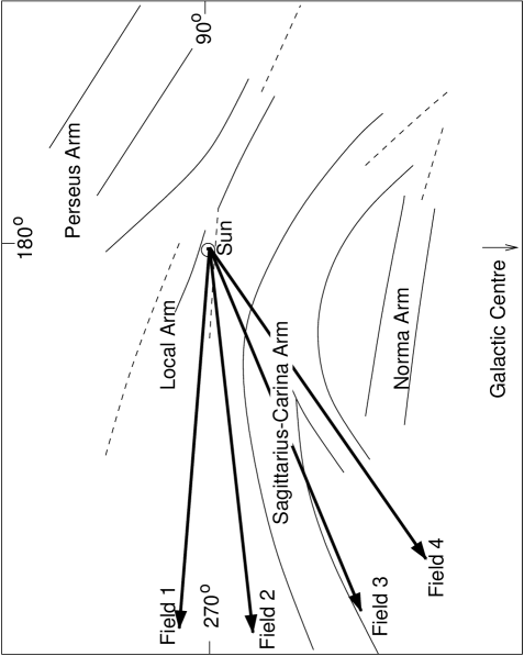
Figure 12: The position of the four fields with respect to the Galactic structure (Humphreys (1976)). F3 and F4 point towards the Sgr-Car arm, whereas no spiral arm is present in the direction of F1 and F2.

7 Discussing the presence of a spiral arm

As already pointed out in the previous sections, the CMDs of fields F3 and F4 (see Fig. 3) show the presence of a few stars brighter than V $\sim 15--15.5$ mag for F4 and F3 respectively and bluer than the average main sequence. Stars in this part of the CMD can be interpreted as tracers of a very young population located in a spiral arm. The idea of a spiral arm is strongly supported by the fact that we find this young population in the fields F3 and F4, which are in the direction of the Sgr-Car arm (see Fig. 1 and 12), whereas the fields F1 and F2, which are not expected to cross the spiral arm, do not show any evidence for such a population.

The spiral arm has been parameterized following Vallee (1995) where however the parameters of the spiral pattern are set to reproduce our data. We adopt an arm/inter-arm density ratio of 2 as found in external galaxies (Rix & Zaritsky 1995) and suggested for our own Galaxy by Efremov (1997). The spiral arm is supposed to have a Gaussian distribution with a $\sigma$ of 300 pc as suggested by Taylor & Cordes (1993), and Vallee (1995). We impose that the age of the spiral arm population is younger than 1 $\times 10^{8}$ y. From CMD simulations, we find out that the faintest magnitude of the blue population gives hints about the distance of the spiral arm from us (see Fig 4). We find out that the distance of the spiral arm in the direction of F3 is about 1.3 $\pm 0.1$ kpc, with the maximum of the distribution at 2 kpc. In the direction of F4, we find that the spiral arm is at a distance of 1.5 $\pm 0.2$ kpc. These results are of course dependent on the adopted parameterization of the spiral arm. They are consistent with the spiral arm pattern defined by the pulsar distribution (Taylor & Cordes (1993)) or derived from optical observations for the local solar environment (Humphreys (1976)).

8 Conclusions

Deep CCD photometry in the V and I pass-bands is presented for 4 low latitude Galactic fields. The studied fields are located between l=265 and l=305.

The scale height and the scale lenght of the various populations are derived. The data seem to favor a disk scale height around $h_{z}=250\pm 0.60\rm\,pc$ and a scale lenght $>$ 1100 pc. The star formation seems to have been decreasing in time, while a constant or increasing star formation rate as the one found using Hipparcos data in the solar neighborhood, cannot reproduce the features of the CMDs: too many blue stars are expected.

From the star-counts in the studied fields we derive the local mass density in stars more massive than 0.1 M_⊙, found to be in the range 0.036-0.022 M_⊙ pc${}^{-}3$.

In two fields, namely F3 and F4 located at l=292 and l=305 evidence is found of the presence of a very young population. The data can be reproduced imposing the presence of a spiral arm. In these direction the Sgr-Car arm is crossed at a distance of 1.3$\pm 0.1$ and 1.5 $\pm 0.2$ Kpc respectively. These results are consistent with previously defined spiral arm patterns (Taylor & Cordes (1993); Humphreys (1976)).

Due to the small field of view, two of the studied fields, F1 and F2 do not set strong constrains on the scale height and the scale lenght of the disk. A larger field of view (see e.g. the WFI at the 2.2m ESO telescope having 30${}^{\prime}\times$ 30^′) would allow us to have good statistics down to faint magnitudes. At l=305, b=-4.8 more than 10⁴ disk stars down to V=21 are expected in such a large field. In a forthcoming paper we will discuss the Galactic structure towards the center making use of the good statistics of the WFI data.

- (1) Bertelli, G., Betto, R., Bressan A., Chiosi, C., Nasi, E., Vallenari, A., 1990, A&AS 85, 845
- (2) Bertelli, G., Bressan, A., Chiosi, C., Ng, Y.K., Ortolani, S., 1995, A&A, 301, 381
- (3) Bertelli G., Bressan A., Chiosi C., Ng Y.N., 1996, A&A 310, 771
- Bertelli et al. (1999) Bertelli G., Bressan A., Chiosi C., Vallenari A., 1999, Balt. Astr., 8, 271
- (5) Bessel, M.S., Stringfellow G.S., 1993, ARA&A 31, 433
- (6) Binney, J., Gerhard O., Spergel D., 1997, MNRAS, 288, 365
- (7) Bressan, A., Fagotto, F., Bertelli, G., Chiosi C., 1993, A&AS 100,647
- (8) Burton W., B., 1988, In Galactic and Extragalactic Radio Astronomy, eds. G.L. Verschuur, K.I. Kellerman, Springer, Berlin.
- (9) Carraro G., Chiosi C., 1994, A&A 287, 761
- (10) Carraro G., Vallenari A., Girardi L., Richichi A., 1999, A&A 343, 825
- (11) Casertano S., Ratnatunga K.U., Bahcall J.N., 1990, ApJ 357, 435
- (12) Chen B., 1996, A&A 306, 733
- (13) Cohen, M.,1995, ApJ 444, 874
- (14) Combes F., 1991, ARA&A, 29, 195
- (15) Creze M., Chereul E., Bienayme O., Pichon C., 1998 A&A 329, 920
- (16) Cunha, K., Lambert, D.L., 1992, ApJ 399, 586
- (17) Diplas A., Savage B.D. 1991, ApJ 377, 126
- (18) Eaton, N., Adams D.J., Giles A.B., 1984, MNRAS, 208, 241
- (19) Efremov Y.N, 1997, Ast.L. 23, 579
- (20) Evardson B., Andersen J.,, Gustafsson B., et al, 1993, A&A 275, 101
- (21) Fagotto, F., Bressan A., Bertelli G., Chiosi C., 1994a, A&AS 105,29
- (22) Fagotto, F., Bressan, A., Bertelli G., Chiosi C., 1994b, A&AS 104, 365
- (23) Fagotto, F., Bressan A., Bertelli G., Chiosi, C., 1994c, A&AS 105, 39
- (24) Friel, E.D., Janes, K.A., 1993, A&A 267, 75
- (25) Freundenreich, H. T.,1996, ApJ 468, 663
- (26) Fux R., Martinet L., 1994, A&A 287, L21
- (27) Gilmore G.,1984, MNRAS 207, 223
- (28) Gilmore G., Reid N.,1983, MNRAS 207, 223
- (29) Gilmore G., Wyse R.F.G., Jones J.B., 1995. AJ 109, 1095
- (30) Girardi L., Bressan A., Chiosi C., Bertelli G., Nasi E., 1996, A&AS 117,113
- (31) Gould A., Bahcall J.N., Maoz D., Yanny B., 1995, ApJ 441, 200
- (32) Hammersley P.L., Gargon F., Mahroney T., Calbet X.,1995, MNRAS, 273, 206
- (33) Haywood M., Robin, A.C., Creze M., 1997, A&A 320, 440
- (34) Hoffmann, B., Tappert, C., Schlosser, W., Schmidt-Kaler, Th., Kimeswenger, S., Seidensticker, K., Schmidtobreick, L., Hovest, W., 1998, A&AS
- Humphreys (1976) Humphreys, R.M., 1976, PASP 88, 647
- (36) Humphreys R.M., Larsen, J.A., 1995, AJ 110, 2183
- (37) Jimenez R., Flynn C., Kotoneva E., 1998, MNRAS 299, 515
- (38) Jones , T.J., Ashley, M., Hyland A.R., Ruelas-Mayorga A. 1981, MNRAS 197, 413
- (39) Kimeswenger, S., Hoffmann, B., Schlosser, W., Schmidt-Kaler, Th., 1993, A&AS, 97, 517
- (40) Kroupa P., 2000, AGM,16, T11
- (41) Landolt, A.U., 1992, AJ, 104, 340
- Mendez & van Altena (1998) Mendez R.A., van Altena, W.F., 1998, A&A 330, 910
- (43) Morrison H.L., Flynn C., Freeman K.C., 1990, AJ 100, 1191
- (44) Norris J.,1987, AJ 93, 616
- Ng et al., (1995) Ng, Y.K., Bertelli, G., Bressan, A., Chiosi, C., Lub, J., 1995, A&A, 295, 655
- (46) Oort J.H., 1960, BAN 15 45
- (47) Phelps, R.,L., 1997, ApJ 483, 826
- (48) Quinn P.J., Hernquist L., Fullagar D.P., 1993, AJ 403, 74
- (49) Reid, N.I., Majewski, S.R., 1993, ApJ 409, 635
- (50) Rix H.W., Zaritsky D., 1995, ApJ 447,82
- (51) Robin A.C., Creze M., Mohan V., 1992, A&A 253, 389
- (52) Robin A.C., Haywood M., Creze M., Ojha D.K., Bienayme O., 1995, A&A 305, 125
- (53) Ruelas-Mayorga R.A., 1991, Rev. Mexicana Astron. Astrphys. 22, 27
- (54) Ruiz, M.T., 1996, AJ 111, 1267
- (55) Sandage A., Fouts, 1987, AJ 93, 74
- (56) Stobie R.S., Ishida, K., 1987, AJ 93, 624
- (57) Schlegel, David J., Finkbeiner, Douglas P., Davis, Marc, 1998, ApJ 500 ,525
- (58) Schlosser, W., Hohl, H., Hovest, W., 1995, Astr.Ges.Abstr.Ser., 11, 190
- (59) Scott, J. E., Friel, E. D., Janes, K. A., 1995, AJ 109, 1706
- Taylor & Cordes (1993) Taylor J.H., Cordes J.M., 1993, ApJ 411, 674
- (61) Tripicco, M. J., Bell, R. A., Dorman, B., Hufnagel, B., 1995, AJ 109, 1697
- (62) Twarog, B.A., 1980, ApJ 242, 242
- (63) Twarog, B.A., Antony-Twarog, B.J., 1994, AJ 107, 1371
- Vallee (1995) Vallee J.P., 1995, ApJ 454, 119
- (65) Wyse, R.F.G., Gilmore, G., 1992, AJ 104, 144