Hierarchical Galaxy Formation

Abstract

We describe the GALFORM semi-analytic model for calculating the formation and evolution of galaxies in hierarchical clustering cosmologies. It improves upon, and extends, the earlier scheme developed by Cole et al. ([1994]). The model employs a new Monte-Carlo algorithm to follow the merging evolution of dark matter halos with arbitrary mass resolution. It incorporates realistic descriptions of the density profiles of dark matter halos and the gas they contain; it follows the chemical evolution of gas and stars, and the associated production of dust; and it includes a detailed calculation of the sizes of disks and spheroids. Wherever possible, our prescriptions for modelling individual physical processes are based on results of numerical simulations. They require a number of adjustable parameters which we fix by reference to a small subset of local galaxy data. This results in a fully specified model of galaxy formation which can be tested against other data. We apply our methods to the $\Lambda$CDM cosmology ($\Omega_{0}=0.3$, $\Lambda_{0}=0.7$), and find good agreement with a wide range of properties of the local galaxy population: the B-band and K-band luminosity functions, the distribution of colours for the population as a whole, the ratio of ellipticals to spirals, the distribution of disk sizes, and the current cold gas content of disks. In spite of the overall success of the model, some interesting discrepancies remain: the colour-magnitude relation for ellipticals in clusters is significantly flatter than observed at bright magnitudes (although the scatter is about right), and the model predicts galaxy circular velocities, at a given luminosity, that are about 30% larger than is observed. It is unclear whether these discrepancies represent fundamental shortcomings of the model or whether they result from the various approximations and uncertainties inherent in the technique. Our more detailed methods do not change our earlier conclusion that just over half the stars in the universe are expected to have formed since $z\la 1.5$.

1 Introduction

The past few years have been a remarkably rich period in observational studies of galaxy formation. Major advances have resulted from observations at many wavelengths, from the far ultraviolet to the sub-millimeter. Breakthroughs include the discovery and measurement of the clustering of “Lyman-break” galaxies, a population of luminous, star-forming galaxies at redshifts $z\sim 3-4$ (Steidel et al. [1996]; Adelberger et al. [1998]); estimates of the history of star formation and the attendant production of metals, from $z\sim 5$ to the present (Madau et al. [1996],[1998]); measurements of the galaxy luminosity function at $z\sim 0.5-1$ ([1996, 1996]) and $z\sim 3-4$ ([1999]); the discovery of a population of bright sub-millimeter sources, some of which, at least, appear to be dusty, star-forming galaxies at $z\ga 2$ ([1998]). All of these and many other observations are beginning to sketch out an empirical picture of galaxy evolution.

On their own, the data provide only a partial description of specific stages of galaxy evolution. To develop a physical understanding of the processes at work, and to relate observations to cosmological theory, requires detailed modelling that exploits our current understanding of astrophysical processes in their cosmological context. The theoretical infrastructure required for this programme has been in place for over a decade (e.g. [1984, 1985]). In its standard form, it assumes that galaxies grew out of primordial Gaussian density fluctuations generated during inflation and amplified by gravitational instability acting on cold dark matter, the dominant mass component of the Universe. Gas is initially mixed in with the dark matter, and when dark matter halos collapse, the visible component of galaxies accumulates as stars condense out of gas that has cooled onto a disk.

To construct a theory of galaxy formation that can be tested against observations requires combining the theory of the evolution of cosmological density perturbations with a description of various astrophysical processes such as the cooling of gas in halos, the formation of stars, the feedback effects on interstellar gas of energy released by young stars, the production of heavy elements, the evolution of stellar populations, the effects of dust, and the merging of galaxies. The most appropriate methodology is to carry out ab initio calculations that follow directly the development of primordial density fluctuations into luminous galaxies. Within the standard cosmological model, the initial conditions are very well defined. They are specified by the power spectrum of primordial density perturbations, whose shape is fixed by the cosmological parameters: the mean mass density, $\Omega_{0}$, the mean baryon density, $\Omega_{\rm b}$, the cosmological constant, $\Lambda_{0}$, and the Hubble constant, $H_{0}$ (which, throughout this paper, we express as $H_{0}=100h{\rm\ kms}^{-1}{\rm Mpc}^{-1}$.)

The subsequent evolution of the dark matter and baryons is best calculated by Monte Carlo simulation. Two different approaches have been developed for this purpose. In the first, direct simulations, the gravitational and hydrodynamical equations in the expanding universe are solved explicitly, using one or more of a variety of numerical techniques that have been specifically developed for this purpose over the past twenty years (e.g. [1992, 1994, 1996], [1999]; [1996, 1997, 1999, 2000, 2000]). In the second approach, now commonly known as “semi-analytic modelling of galaxy formation” ([1978, 1991, 1993, 1994]), the evolution of the baryonic component is calculated using simple analytic models, while the evolution of the dark matter is calculated either directly, using N-body methods, or using a Monte-Carlo technique that follows the formation of dark matter halos by hierarchical merging. It is this second approach that we discuss in this paper.

The two modelling techniques have complementary strengths. The major advantage of direct simulations is that the dynamics of the cooling gas are calculated in full generality, without the need for simplifying assumptions. The main disadvantage is that even with the best codes and fastest computers available today, the attainable resolution is still some orders of magnitude below that required to resolve the formation and internal structure of individual galaxies in cosmological volumes. In addition, a phenomenological model, similar to that employed in semi-analytic modelling, is required to include star formation and feedback processes in the simulation. These processes are, in fact, much more difficult to treat and much more uncertain than the dynamics of the diffuse gas.

Semi-analytic modelling does not suffer from resolution limitations, particularly when Monte-Carlo methods are used to generate the halo merger histories. In this case, the resolution can be made arbitrarily high at a relatively small computational cost. The major disadvantage is the need for simplifying assumptions in the calculation of gas properties, such as spherical symmetry or a particular flow structure. It is encouraging that detailed comparisons between direct and semi-analytic simulations show good agreement (Pearce et al. [1999], Benson et al. [2000c]). An important advantage of semi-analytic modelling is its flexibility. This allows the effects of varying assumptions or parameter choices to be readily investigated and makes it possible to calculate a wide range of observable galaxy properties, such as luminosities in any waveband, sizes, mass-to-light ratios, bulge-to-disk ratios, circular velocities, etc.

Semi-analytic modelling has its roots in the work of White & Rees ([1978]), Cole ([1991]), Lacey & Silk ([1991]), and White & Frenk ([1991]) who laid out the overall philosophy and basic methodology of this approach. Throughout most of the 1990s, this technique was developed and promoted primarily by two collaborations, one currently based at Munich (e.g. Kauffmann et al. [1993],[1994] Kauffmann [1995a],b, Kauffmann, Nusser & Steinmetz [1997], Mo, Mao & White [1998a],b,[1999], Kauffmann et al. [1999a] ), and the other at Durham (e.g. Cole et al. [1994], Heyl et al. [1995], Baugh et al. [1996a],b, [1998], Benson et al. [2000a]; see also Lacey et al. [1993]). In the past two years, several other groups have begun to apply this technique to study various aspects of galaxy formation (e.g. Avila-Reese & Firmani [1998], Guiderdoni et al. [1998], Wu, Fabian & Nulsen [1998], van Kampen, Jimenez & Peacock [1999], Somerville & Primack [1999]). This body of work has demonstrated the usefulness of semi-analytic modelling as a means for fleshing out the observable consequences of current cosmological theories and for the interpretation of observational data, particularly at high redshift.

A growing body of galaxy properties has been analysed using semi-analytic methods. Examples of noteworthy successes include the ability to reproduce the local field galaxy luminosity function, the slope and scatter of the Tully-Fisher relation for spiral galaxies, and the counts and redshift distributions of faint galaxies (e.g. see [1993, 1994, 1994]). Nevertheless, some important properties have remained obstinately difficult to reproduce, most notably the colour-magnitude relation for cluster ellipticals (but see Kauffmann & Charlot [1998a]) and a simultaneous fit to the local luminosity function and the zero-point of the Tully-Fisher relation (e.g. Heyl et al. [1995]).

Figure 1: A schematic showing how different physical processes are combined to make predictions for the observable properties of galaxies, starting from initial conditions specified by the cosmology. The numbers in each box indicate the subsection of the paper in which our method for modelling that process is described.

Figure 2: A schematic showing the observable galaxy properties predicted by the model. The numbers in each box indicate the subsection of the paper in which the comparison of model predictions with observations of that property are described. The predictions for galaxy clustering are described in separate papers, as indicated in the box.

A wide variety of physical processes are involved in the formation of galaxies. Some of them, like star formation, are very poorly understood. Modelling galaxy formation therefore inevitably requires making approximations and adopting simplified descriptions of some of these processes. Most often, an incomplete understanding of a physical ingredient is subsumed within a simple scaling law that contains free parameters. A remarkable facet of modern semi-analytic modelling is that a realistic picture of galaxy evolution can be formulated with a relatively small number of such parameters, typically four or five in the simplest versions. A strategy that has proved useful is to fix the values of these parameters by trying to match a subset of local data (for example, the luminosity functions in two passbands or the Tully-Fisher relation). This leads to a completely specified model that has predictive power and may be used to calculate theoretical expectations for other local properties or for properties at high redshift. This approach has met with considerable success. For example, Cole et al. ([1994]) predicted that most of the stars in the universe formed at relatively low redshift ($z\la 1$ for an $\Omega_{0}=1$ standard CDM cosmology); Kauffmann ([1996]) predicted a sharply declining number of bright elliptical galaxies at high redshift; and Baugh et al. ([1998]) and Governato et al. ([1998]) predicted strong clustering for Lyman-break galaxies at redshift $z\simeq 3$.

In this paper we present a new semi-analytic model which builds upon the scheme described by Cole et al. ([1994]) which we used for a number of applications (Heyl et al. [1995], Baugh et al. [1996a]b). Our new model differs from the earlier one primarily in its greater scope and richness, but also in the manner in which certain key physical properties are calculated. These improvements are called for both by recent theoretical developments and, most importantly, by the increase in the quantity and quality of observational data. The main additions to our new code are the inclusion of chemical enrichment and dust processes, prescriptions for calculating the sizes of disks and spheroids, the use of more realistic density profiles for dark matter halos and gas, and the ability to follow the mergers of halos with fine mass and time resolution. It should be noted that despite all these improvements, when one adopts the same cosmological parameters and also the same galaxy formation parameters (e.g. for stellar feedback), then the main predictions of the model, including the galaxy luminosity function, Tully-Fisher relation and overall star formation history, are practically identical to those in Cole et al. ([1994]). The one exception is the inclusion of dust extinction which makes the galaxy colours somewhat redder than in the Cole et al. ([1994]) models. Thus, the changes to the model may be viewed as refinements that allow more properties of the galaxy population, such as galaxy sizes and metallicities, to be calculated.

The main aim of this paper is to lay out the methods that we use in our new semi-analytic model and to compare results with a restricted set of observational data. This is a long paper containing a mixture of technical descriptions and results of more general interest. In the following, brief section, we present an overview, together with schematics illustrating how different parts of the model fit together. Non-specialist readers may wish to skip the more detailed passages of the paper on a first reading and we recommend how this might done in Section 2.

2 Overview

Our galaxy formation model is a synthesis of many techniques, each of which has been developed to treat particular aspects of the complex process of galaxy formation. Its backbone is a Monte Carlo method for generating “merger trees” to describe the hierarchical growth of dark matter halos. The full range of properties and processes that we model within this framework are:

1. The gravitationally-driven formation and merging of dark matter halos.

2. The density and angular momentum profiles of dark matter and shock heated gas within dense non-linear halos.

3. The radiative cooling of gas and its collapse to form centrifugally supported disks.

4. The scalelengths of disks based on angular momentum conservation and including the effect of the adiabatic contraction of the surrounding halo during the formation of the disk.

5. Star formation in disks.

6. Feedback, i.e. the regulation of the star formation rate resulting from the injection of supernova (SN) energy into the interstellar medium (ISM).

7. Chemical enrichment of the ISM and hot halo gas and its influence on both the gas cooling rates and the properties of the stellar populations that are formed.

8. The frequency of galaxy mergers resulting from dynamical friction operating on galaxies as they orbit within common dark matter halos.

9. The formation of galactic spheroids, accompanied by bursts of star formation, during violent galaxy-galaxy mergers, and estimates of their effective radii.

10. Spectrophotometric evolution of the stellar populations.

11. The effect of dust extinction on galaxy luminosities and colours, and its dependence on galaxy inclination.

12. The generation of emission lines from interstellar gas ionized by young stars.

Our treatment of each of these processes is described in the following sections. The model is summarized schematically in Fig. 1, which also shows in which subsection of the paper each of the processes is described.

The scheme we present is largely modular, and within each module one has the choice of selecting various options as well as certain parameter values. The options (for example, including or ignoring the baryonic mass of the galaxy when computing its rotation curve) are not degrees of freedom within the model. Instead they allow us to vary the complexity of the description in order to gain physical understanding. By switching processes on and off and changing certain assumptions we are able to determine which physical processes are directly responsible for a particular galaxy property.

The observable galaxy properties predicted by the model are shown schematically in Fig. 2. This figure separates the predicted quantities into two categories. Some aspects of the observational quantities in the first category are used as primary constraints on the model parameters. The boxes in the figure also indicate in which subsection of the paper the observational comparison for that quantity is presented, or in the case of galaxy clustering, the related papers in which they are presented. Predictions for the redshift evolution of galaxy properties will be presented in future papers.

The layout of the paper is as follows: Section 3 presents techniques for generating merger trees to describe the gravitational growth of dark matter halos and models for their internal structure. Section 4 describes how we calculate disk and spheroid formation, including star formation, feedback and chemical evolution, and the scalelengths of galactic disks and bulges. Section 5 presents our methods for calculating the luminosities of stellar populations, and the effects of dust extinction. These three sections may be skipped on a first reading, simply noting the definition of the parameters that describe our star formation and feedback model, equations (4.13), (4.14), (4.23), and (4.24). An overview of the model and the strategy we adopt to constrain parameters and to obtain a well-specified, predictive model are presented in Section 6, which should be of general interest. This procedure is implemented in Section 7, where we illustrate the effects of varying each model parameter. The general reader may simply wish to study the figures in this section and read the summary in subsection 7.9. In Section 8 we test our fully specified model against further properties of the observed galaxy population. Again, the general reader may wish to study only the figures in this section. Finally, in Section 9 we restate the general philosophy of our approach and discuss the strengths and weaknesses of the specific model that we have presented. This, and the final section presenting a summary of our results, are both of general interest.

3 Formation of Dark Matter Halos

Galaxies are assumed to form inside dark matter halos, and their subsequent evolution is controlled by the merging histories of the halos containing them. It is therefore essential to have an accurate description of how dark halos form and evolve through hierarchical merging, and of the internal structure of these halos. These are both described in this section.

3.1 Dark Matter Halo Merger Trees

We use a new Monte-Carlo algorithm to generate merger trees that describe the formation paths of randomly selected dark matter halos. It is an improvement over the “block model” that we used previously ([1994, 1995, 1996a],b). The new algorithm is directly based on the analytic expression for halo merger rates derived by Lacey & Cole ([1993]). At each branch in the tree, a halo splits into two progenitors, but unlike in the “block model”, the mass ratio of the progenitors can take any value. Below, we briefly describe this new algorithm, and the way in which a population of merger trees is set up to provide a framework for modelling the processes of galaxy formation.

It is possible to generate merger trees directly by following the evolution of dark matter halos in collisionless cosmological N-body simulations (e.g. Roukema [1997]; Kauffmann et al. [1999a]; van Kampen et al. [1999]). Combining semi-analytic modelling and N-body simulations certainly provides a very powerful technique to investigate small scale galaxy clustering (e.g. Kauffmann, Nusser & Steinmetz [1997], Governato et al. [1998], Kauffmann et al. [1999a],b, Benson et al. [2000a],b). However, extracting merger trees directlty from N-body simulations carries the high price of a limited dynamic range in mass and much greater computational complexity. Also, for many applications this appears to be unnecessary, as the properties of halo merger trees are uncorrelated with environment (Lemson & Kauffmann [1999]), and the Monte Carlo merger trees agree well, statistically, with those extracted from N-body simulations ([1993, 1994, 2000]; Lacey & Cole in preparation).

3.1.1 A New Algorithm

Our starting point for generating a merger tree to describe the history of mergers experienced by an individual dark matter halo is equation (2.15) of Lacey & Cole ([1993]):

$$f_{12}(M_{1},M_{2})dM_{1}\negthinspace = \negthinspace\negthinspace\frac{1}{\sqrt{2\pi}}\ \frac{(\delta_{\rm c1}-\delta_{\rm c2})^{{\hphantom{3/2}}}}{(\sigma_{1}^{2}-\sigma_{2}^{2})^{3/2}}$$ (3.1)

$$\times \negthinspace\negthinspace\exp\left(-\frac{(\delta_{\rm c1}-\delta_{\rm c2})^{2}}{2(\sigma_{1}^{2}-\sigma_{2}^{2})\hphantom{2}}\right)\frac{d\sigma_{1}^{2}}{dM_{1}}dM_{1}.$$

This equation, derived from the extension of the Press & Schechter ([1974]) theory proposed by Bond et al. ([1991]) and Bower ([1991]), gives the fraction of mass, $f_{12}(M_{1},M_{2})dM_{1}$, in halos of mass $M_{2}$, at time $t_{2}$, which at an earlier time, $t_{1}$, was in halos of mass in the range $M_{1}$ to $M_{1}+dM_{1}$. Here, the quantities $\sigma_{1}$ and $\sigma_{2}$ are the linear theory rms density fluctuations in spheres of mass $M_{1}$ and $M_{2}$. The $\delta_{\rm c1}$ and $\delta_{\rm c2}$ are the critical thresholds on the linear overdensity for collapse at times $t_{1}$ and $t_{2}$ respectively. (Specifically, $\sigma(M)$ and $\delta_{\rm c}(t)$ are the values extrapolated to $z=0$ according to linear theory.) For a critical density ($\Omega=1$) universe, we adopt $\delta_{\rm c}=1.686(1+z)$, while for low $\Omega_{0}$, open and flat, universes we adopt the appropriate expressions in the appendices of Lacey & Cole ([1993]) and Eke, Cole & Frenk ([1996]) respectively.

Equation (3.1) can be used to estimate the recent merger histories of a set of halos which at time $t_{2}$ have mass $M_{2}$. Taking the limit of equation (3.1) as $t_{1}\rightarrow t_{2}$, we obtain an expression for the average mass fraction of a halo of mass $M_{2}$ which was in halos of mass $M_{1}$ at the slightly earlier time $t_{1}$,

$$\frac{df_{12}}{dt_{1}}\Big{|}_{t_{1}=t_{2}}\negthinspace\negthinspace\negthinspace\negthinspace\negthinspace\negthinspace\negthinspace dM_{1}dt_{1}=\frac{1}{\sqrt{2\pi}}\frac{1}{(\sigma_{1}^{2}-\sigma_{2}^{2})^{3/2}}\frac{d\delta_{\rm c1}}{dt_{1}}\frac{d\sigma_{1}^{2}}{dM_{1}}dM_{1}dt_{1}.$$ (3.2)

Thus, the mean number of objects of mass $M_{1}$ that a halo of mass $M_{2}$ “fragments into” when one takes a step $dt_{1}$ back in time is given by

$$\frac{dN}{dM_{1}}=\frac{df_{12}}{dt_{1}}\frac{M_{2}}{M_{1}}dt_{1}\qquad\qquad\qquad(M_{1}<M_{2}).$$ (3.3)

This expression gives the average number of progenitors as a function of the fragment mass, $M_{1}$. It is this simple expression that our algorithm uses to build a binary merger tree.

The quantities that must be specified in order to define the merger tree are the density fluctuation power spectrum, which gives the function $\sigma(M)$, and the cosmological parameters, $\Omega_{0}$ and $\Lambda_{0}$, which enter through the dependence of $\delta_{c}(t)$ on the cosmological model. There is also one numerical parameter involved, the mass resolution, $M_{\rm res}$. Having specified these parameters one can compute the two quantities,

$$P=\int_{M_{\rm res}}^{M_{2}/2}\frac{dN}{dM_{1}}dM_{1},$$ (3.4)

which is the mean number of fragments with masses, $M_{1}$, in the range $M_{\rm res}<M_{1}<M_{2}/2$, and

$$F=\int_{0}^{M_{\rm res}}\frac{dN}{dM_{1}}\frac{M_{1}}{M_{2}}dM_{1},$$ (3.5)

which is the fraction of mass in fragments with mass below the resolution limit. Note that both these quantities are proportional to the timestep $dt_{1}$, through the dependence in equation (3.3).

Once these quantities have been defined, the algorithm to generate the merger trees is simple. First, choose a timestep, $dt_{1}$, such that $P\ll 1$, to ensure that multiple fragmentation is unlikely. Next, generate a random number, $R$, drawn uniformly from the interval 0 to 1. If $R>P$, then the main halo does not fragment at this timestep. However, the original mass is reduced to account for mass accreted in the form of halos with masses below the resolution limit, to produce a new halo of mass $M_{2}(1-F)$. If, however, $R<P$, then a random value of $M_{1}$ in the range $M_{\rm res}<M_{1}<M_{2}/2$ is generated, consistent with the distribution given by equation (3.3), to produce two new halos with masses $M_{1}$ and $M_{2}(1-F)-M_{1}$. The same operation is repeated on each fragment at successive timesteps going back in time, and thus a merger tree is built up.

The main advantage of this new algorithm over the “block model” that we used previously ([1994, 1995, 1996a]b), and which has been used recently by Wu et al. ([1998],[2000]), is that there is no quantization of the progenitor halo masses. The algorithm also enables the merger process to be followed with high time resolution, as timesteps are not imposed on the tree but rather are controlled directly by the frequency of mergers. It is similar in spirit to the method used by Kauffmann et al. ([1993]), but has several advantages, including smaller timesteps and not having to store large tables of progenitor distributions. Somerville & Kolatt ([1999]) investigated a similar algorithm also based on equation (3.1), which they referred to as binary mergers without accretion. They rejected that algorithm as it over-predicted the number of massive halos at high redshift, and instead opted for a more elaborate algorithm which they compared with N-body simulations in Somerville et al. ([2000]). Our algorithm, which we first used in Baugh et al. ([1998]), differs from the one they rejected in two important respects. First, we explicitly account for accretion of objects below the mass resolution using the expression (3.5). Second, we make the rather subtle choice of selecting the first progenitor mass, $M_{1}$, only in the range $M_{\rm res}<M_{1}<M/2$ of the distribution defined by (3.3). We have found, that together, these choices produce an algorithm that successfully produces distributions of progenitors which, on average, agree quite accurately with the analytic expressions given by the extended Press-Schechter theory. Moreover, statistics that are not predicted by the extended Press-Schechter theory, such as the frequency distribution of progenitors of a given mass (the extended Press-Schechter theory only predicts the mean of the distribution), we find to be in excellent agreement with the same statistics extracted from N-body simulations. This detailed investigation of the behaviour of the algorithm will be presented in a future paper (Lacey & Cole in preparation).

3.1.2 Utilizing the Merger Trees

Although the merger trees described above have very high time resolution, the nature of the galaxy formation rules that we implement below require placing the merger tree onto a predefined grid of timesteps. The original binary merger tree is used to find which halos exist at each timestep and to identify which of them merge together between timesteps. As a consequence, mergers that are actually rapid, consecutive binary mergers in the original tree will appear as simultaneous, multiple mergers in the discretized tree. The loss of information involved is not significant since, in reality, mergers are not instantaneous events and our discrete timesteps are typically much smaller than the dynamical timescales of the merging halos. Each merger tree thus starts from a single halo of a specified mass $M$ at $z=z_{\rm halo}$, where $z_{\rm halo}$ is the redshift for which we want to calculate the galaxy properties. It extends up to some earlier redshift $z_{\rm start}>z_{\rm halo}$, where the tree has split into many branches. The generation of the halo merger tree proceeds backwards in time, starting from the trunk at $z=z_{\rm halo}$, but the calculation of galaxy formation and evolution through successive halo mergers proceeds forwards in time, moving down from the top of the tree. The appropriate grid of $N_{\rm steps}$ timesteps, the starting redshift $z_{\rm start}$ and also the mass resolution, $M_{\rm res}$, depend on the problem of interest. The timesteps can, for example, be chosen to be uniform either in time or in the logarithm of the cosmological expansion factor. For the models presented here, we typically set $M_{\rm res}=5\times 10^{9}h^{-1}M_{\odot}$ and use $100$ timesteps logarithmically spaced in expansion factor between $z=0$ and $7$. In our models, stellar feedback prevents significant amounts of star formation occurring in halos of very low circular velocity and so provided $M_{\rm res}$ is sufficiently low, the model results are not affected by its value.

The second way in which we manipulate the merger trees before applying our galaxy formation rules is by chopping each tree into branches that define the formation time and lifetime of each halo. So far we have done this using a simple algorithm. We start, at the first timestep, at the top of the tree (corresponding to the lowest mass halos in the merging hierarchy), and define each halo present as a new halo that formed at that timestep. We then follow each of these halos through their subsequent mergers until they have become part of a halo with mass greater than $f_{\rm form}$ times the original mass. We normally set $f_{\rm form}=2$. This point defines the end of the original halo’s lifetime. Consistent with this definition, the point at which a new halo life begins is defined by the point when mergers produce a halo whose mass exceeds $f_{\rm form}$ times the formation mass of its largest progenitor. When applying the galaxy formation rules detailed in the following sections, we always treat the halos as if they retained, throughout their lifetime, the mass and other properties, (mean density, angular momentum, etc.) with which they formed. The mass accreted prior to the final merger, which can, in extreme cases, be as large as $f_{\rm form}-1$ times the original halo mass, is effectively treated as if it were all accreted at the end of the halo’s lifetime. We have chosen $f_{\rm form}=2$ for consistency with our earlier work (Cole et al. [1994]) in which a factor of two was built into the “block model” that we used to generate merger trees. With this choice the two models produce near identical results when the content and parameters of the galaxy formation model are the same. In Table 3 of Section 7.1, we include one variant model with $f_{\rm form}=1.5$ which demonstrates that the model is not very sensitive to the choice of this parameter. This is natural as most halos end their lives when they are accreted onto much more massive halos and thus their lifetimes are robust to the choice of $f_{\rm form}$.

In order to investigate the statistical properties of galaxy populations, we generate a set of merger trees starting from a grid of parent halo masses specified at some redshift, $z_{\rm halo}$. For each given halo mass, we generate many realizations of the merger tree. The resulting model galaxies can then be sampled, taking account of the abundance of the parent halos at $z=z_{\rm halo}$, to construct galaxy catalogues with any desired selection criteria such as an absolute or apparent magnitude limit. Alternatively, properties such as the galaxy luminosity function or number counts can be estimated directly by a weighted sum over the model galaxies. We have used the Press-Schechter mass function to estimate the halo abundance, but it is well known that this formula overestimates the abundance of $M_{\star}$ objects somewhat (e.g. Efstathiou et al. [1988]; Lacey & Cole [1994]). Recently, Sheth, Mo & Tormen ([2000]) and Jenkins et al. ([2000]) have presented fitting formulae that match the results of N-body simulations to high accuracy. In future it will be preferable to use these formulae, but here we simply note that adopting the Jenkins et al. ([2000]) mass function would make little difference to our model predictions.

3.2 Halo Properties

In order to calculate the properties of the galaxies that form within the dark matter halos produced by the merger tree, we need a model for the internal structure of the halos. This must specify the halo rotation velocity required to calculate the angular momentum of the gas that cools to form disks, and the halo density profile required to calculate the sizes and rotation speeds of the galaxies.

The properties of dark matter halos formed in cosmological, collisionless, N-body simulations have been extensively studied (e.g. Frenk et al. [1985], [1988]; Barnes & Efstathiou [1987]; Warren et al. [1992]; Cole & Lacey [1996]; Navarro, Frenk & White [1995a], [1996], [1997]; Moore et al. [1999b], Jing [2000]). The models detailed below are designed to be consistent with the results from these simulations.

3.2.1 Spin Distribution

Dark matter halos gain angular momentum from tidal torques operating during their formation. The magnitude of this angular momentum is conventionally quantified by the dimensionless spin parameter

$$\lambda_{\rm H}=\frac{J_{\rm H}|E_{\rm H}|^{1/2}}{{\rm G}M_{\rm H}^{5/2}},$$ (3.6)

where $M_{\rm H}$, $J_{\rm H}$ and $E_{\rm H}$ are the total mass, angular momentum and energy of the halo. The distributions of $\lambda_{\rm H}$ found in various N-body studies ([1987, 1988, 1992, 1996, 1999]) agree very well with one another. They depend only very weakly on halo mass and on the form of the initial spectrum of density fluctuations.

A good fit to the results of Cole & Lacey ([1996]) is provided by the log-normal distribution,

$$P(\lambda_{\rm H})d\lambda_{\rm H}=\frac{1}{\sqrt{2\pi}\sigma_{\lambda}}\exp\left(-\frac{(\ln\lambda-\ln\lambda_{\rm med})^{2}}{2\sigma_{\lambda}^{2}}\right)\frac{d\lambda_{\rm H}}{\lambda_{\rm H}},$$ (3.7)

with $\lambda_{\rm med}=0.039$ and $\sigma_{\lambda}=0.53$. This fit was obtained specifically for halos with $M_{\star}<M_{\rm H}<2M_{\star}$ in the case of an $n=-2$ power spectrum, which is the most relevant for CDM models on galaxy scales, but we stress that the fit parameters depend only very weakly on mass and on the slope of the power spectrum. For example, this fit also reproduces quite accurately the distribution plotted in Fig.4 of Lemson & Kauffmann ([1999]), which is for galactic mass halos in a $\tau$CDM simulation. We use this distribution to assign, at random, a value of $\lambda_{\rm H}$ to each newly formed halo. Note that we do not take account of a possible correlation between the angular momenta of merging halos. It would be necessary to do this if one wanted to follow the angular momenta of galaxy merger products, but we currently do not attempt this.

3.2.2 Halo density Profile

Our standard choice is to model the dark matter density profile using the NFW model ([1995a]):

$$\rho(r)=\frac{{\Delta_{\rm vir}}\rho_{\rm crit}}{f(a_{\rm NFW})}\ \frac{1}{r/{r_{\rm vir}}\;(r/{r_{\rm vir}}+a_{\rm NFW})^{2}}\quad(r\leq{r_{\rm vir}}),$$ (3.8)

with $f(a_{\rm NFW})=\ln(1+1/a_{\rm NFW})-1/(1+a_{\rm NFW})$, truncated at the virial radius, ${r_{\rm vir}}$. We define the virial radius as the radius at which the mean interior density equals ${\Delta_{\rm vir}}$ times the critical density, $\rho_{\rm crit}=3H^{2}/(8\pi G)$. Here the virial overdensity, $\Delta_{\rm vir}$, is defined by the spherical collapse model which yields $\Delta_{\rm vir}=178$ for $\Omega_{0}=1$. Expressions for $\Delta_{\rm vir}$ in low $\Omega_{0}$, open and flat, universes can be found in the appendices of Lacey & Cole ([1993]) and Eke et al. ([1996]) respectively. Confirmation that this definition of the virial radius is physically sensible is provided by Fig.13 of Cole & Lacey ([1996]) and Fig.10 of Eke, Navarro & Frenk ([1998]). These show that on average the transition between dynamical equilibrium and the surrounding infall occurs close to this radius. The NFW profile has one free parameter, $a_{\rm NFW}$, which is a scalelength measured in units of the virial radius. Allowing this one parameter (equivalent to the inverse of the concentration in the terminology of Navarro et al. ) to vary, the density profile accurately fits the profiles of isolated halos grown in cosmological N-body simulations for a wide range of masses and initial conditions (Navarro et al. [1996],[1997]), including simulations that contain adiabatic gas as well as collisionless dark matter ([1998, 1999]). Furthermore, there is a correlation between the best fit value of $a_{\rm NFW}$ and halo mass. This can be understood in terms of how the typical formation time of a halo depends on mass ([1996]). A simple analytic model for this relation has been presented in the appendix of Navarro et al. ([1997]), and it is this that we use to set the values of $a_{\rm NFW}$ for our halos. Jing ([2000]) and Bullock et al. ([1999]) have found that there is considerable scatter about the mean correlation, which is presumably related to the differing dynamical states and formation histories of the halos. We do not take this into account, but we note that simply including this scatter by randomly perturbing the $a_{\rm NFW}$ values has little effect of the resulting distributions of galaxy properties. For instance, the distribution of galaxy sizes is already broad as a result of its dependence on the very broad distribution of halo angular momenta.

Subsequently to the Navarro et al. ([1997]) paper, there has been some debate as to the accuracy with which the NFW profile fits the very central regions of dark matter halos simulated at very high resolution (Moore et al. [1998]; Kravtsov et al. [1998]). When a concensus is reached it may be possible to improve this aspect of our modelling by adopting a slightly modified density profile. We note that the most recent simulations by Moore et al. ([1999a]) yield density profiles which are slightly more centrally concentrated than the Navarro et al. ([1997]) result. To an accuracy of 20% they can be fitted by NFW profiles, but with the scalelengths, $a_{\rm NFW}$, reduced by a factor of 2/3. Such a change has only a relatively small effect on the galaxy properties that we examine below. The largest changes are to the disk scalelengths, which decrease by 10%, and to the disk circular velocities, which increase by 7.5%.

3.2.3 Halo Rotation Velocity

To compute the angular momentum of that fraction of the halo gas that cools and is involved in forming a galaxy, we need a model of the rotational structure of the halo. We assume that the mean rotational velocity, $V_{\rm rot}$, of concentric shells of material is constant with radius and always aligned in the same direction. This simple description is broadly consistent with the behaviour seen in the simulations of Warren et al. ([1992]) and Cole & Lacey ([1996]). The appropriate value of $V_{\rm rot}$ can be related to the halo spin parameter, $\lambda_{\rm H}$, by evaluating, for the adopted halo model, the quantities defining $J_{\rm H}$ and $E_{\rm H}$ in equation (3.6). This calculation is described in Appendix A. We obtain

$$V_{\rm rot}=A(a_{\rm NFW})\lambda_{\rm H}V_{\rm H},$$ (3.9)

where $V_{\rm H}\equiv(GM/{r_{\rm vir}})^{1/2}$ is the circular velocity of the halo at the virial radius. The dimensionless coefficient $A(a_{\rm NFW})$ is a weak function of $a_{\rm NFW}$, varying from $A\approx 3.9$ for $a_{\rm NFW}=0.01$ to $A\approx 4.5$ for $a_{\rm NFW}=0.3$.

Our code allows us to explore the effects of using alternative dark matter density profiles. In particular, we have included the case of a singular isothermal density profile, $\rho(r)\propto r^{-2}$, and a non-singular isothermal density profile, $\rho(r)\propto 1/((r/{r_{\rm vir}})^{2}+a^{2})$. We find $A=8\sqrt{2}/\pi\approx 3.6$ for the singular isothermal sphere (see Appendix A). The value of $A$ decreases very slowly as a core radius is introduced, falling to $A\approx 3.4$ for $a=0.3$.

Our model of the distribution of hot gas in the halo is described in Section 4.1.1. As the hot gas is less centrally concentrated than the dark matter, if we were to assume they had identical rotation velocities this would result in the gas having a slightly higher mean specific angular momentum than the dark matter. We therefore take the rotation velocity of the gas to also be constant with radius, but with a value $V^{\rm gas}_{\rm rot}$ such the gas and dark matter have the same mean specific angular momentum within the virial radius. This simple model seems to be in reasonable accord with the properties of clusters in the high-resolution, gas-dynamic simulations of Eke et al. ([1998], Eke private communication).

4 Formation of Disks and Spheroids

In this section we describe how disks and spheroids form, how we model star formation, feedback and chemical evolution, and how we calculate galaxy sizes.

4.1 Disk Formation

We assume that disks form by cooling of gas initially in the halo. Tidal torques impart angular momentum to all material in the halo, including the gas, so that gas which has cooled and lost its pressure support will naturally settle into a disk. Below, we detail how we compute the mass of the forming disk based on the radiative cooling rate of the halo gas, and how we compute its angular momentum.

4.1.1 Hot Gas Distribution

Diffuse gas which is not part of galaxies is assumed to be shock-heated during halo collapse and merging events. We will refer to this halo gas as “hot”, to distinguish it from the gas in galaxies, which we call “cold”. To calculate how much of this hot gas cools to form a disk, we need to know its initial temperature and density profile. In contrast to most previous work, we will not assume that the hot gas has the same density profile as the dark matter.

High-resolution hydrodynamical simulations of the formation of galaxy clusters (Navarro et al. [1995a]; Eke, Navarro & Frenk [1998], Frenk et al. [1999]) show that, in the absence of radiative cooling, the resulting dark matter distribution is well-modelled by an NFW profile, but that the shock-heated gas is less centrally concentrated. The gas distribution is well fit by the $\beta$-model ([1976]), $\rho_{\rm gas}(r)\propto(r^{2}+r_{\rm core}^{2})^{-3\beta_{\rm fit}/2}$, traditionally used to model the hot X-ray emitting gas in galaxy clusters. The simulations of Eke et al. ([1998]), which span a narrow range of halo mass in an $\Omega_{0}=0.3$, $\Lambda_{0}=0.7$ cosmology, indicate that the typical cluster gas profile is accurately described by a $\beta$-model with $\beta_{\rm fit}\approx 2/3$ and $r_{\rm core}/r_{\rm NFW}\approx 1/3$. Here, $r_{\rm NFW}$ is the NFW scalelength, equal to $a_{\rm NFW}{r_{\rm vir}}$, and so for these clusters $r_{\rm core}/{r_{\rm vir}}\approx 1/20$. A similar result was found for clusters in an $\Omega_{0}=1$ cosmology by Navarro et al. ([1995a]). In both cases, the simulations produce cluster gas temperature profiles that vary slowly with radius, consistent with hydrostatic equilibrium. The mean temperature of the gas is close to the virial temperature, defined by

$${T_{\rm vir}}=\frac{1}{2}\,{\mu m_{\rm H}\over k}V_{\rm H}^{2},$$ (4.10)

where $m_{\rm H}$ is the mass of the hydrogen atom and $\mu$ the mean molecular mass.

Motivated by these simulation results, we assume that any diffuse gas present in the progenitors of a forming halo is shock-heated during the halo formation process and then settles into a spherical distribution with density profile,

$$\rho_{\rm gas}(r)\propto 1/(r^{2}+r_{\rm core}^{2}).$$ (4.11)

For simplicity, we assume the gas temperature to be constant and equal to the virial temperature, ${T_{\rm vir}}$. The effect this assumption has on the cooling radii and masses, computed below, is generally very small, as the cooling time of the gas depends more strongly on density than temperature and the density gradient is typically much larger than the temperature gradient. Guided also by the numerical simulations, we assume that, for the first generation of halos, $r_{\rm core}=r_{\rm NFW}/3$. However, this result is for simulations which do not include radiative cooling, and we expect this relationship to be modified for halos formed from progenitors in which gas has already been removed by cooling. The gas that is able to cool most efficiently in any halo is the densest gas with the lowest entropy. Thus, the remaining gas involved in the formation of a new halo will have a higher minimum entropy than if cooling had not occured. The analytic work of Evrard & Henry ([1991]), Kay & Bower ([1999]) and Wu et al. ([2000]) suggests that increasing the minimum entropy of the halo gas has the effect of increasing its core radius. Further out, where cooling has had little effect, the gas properties will be less affected and, in particular, the pressure at the virial radius, which is ultimately maintained by shocks from infalling material, will remain unchanged.

As a qualitative description of the behaviour described above we have constructed the following simple model. When a new halo is formed in a merger, if the hot gas fraction in the halo is less than the global value of $\Omega_{\rm b}/\Omega_{0}$ (indicating that some gas has already cooled), we increase the gas core radius, $r_{\rm core}$, until we recover the same density at the virial radius that we would have obtained had no gas cooled. In principle, this ceases to be possible once the gas fraction is so low that even if it were placed in the halo at constant density, this density would be below the target value. To deal with this contingency, we set an upper limit of $r_{\rm core}=10{r_{\rm vir}}$, but in practice this extreme is rarely reached. The result of this procedure, when applied to the models discussed in Section 7, is that at high redshift the core radii start with values close to $r_{\rm core}=r_{\rm NFW}/3$, which for isolated bright galaxies, groups and clusters are approximately $20$,$30$,$50h^{-1}$ kpc respectively. As gas cools and galaxy formation proceeds, the core radii grow until, at the present day, the corresponding median core radii for newly formed halos are $85$, $125$ and $175h^{-1}$ kpc. The distributions of core radii typically span a factor of two in scale.

As alternatives to this standard description, our code also allows us to keep the core radius fixed, either as a fixed fraction of the virial radius or of the NFW scalelength, or even simply to assume that the gas traces the dark matter density profile. These options allow us to gauge directly the effects of our model assumptions.

4.1.2 Cooling

Assuming that the shock-heated halo gas is in collisional ionization equilibrium, the cooling time, defined as the ratio of the thermal energy density to the cooling rate per unit volume, $\rho_{\rm gas}^{2}\Lambda(T_{\rm gas},Z_{\rm gas})$, is

$$\tau_{\rm cool}(r)=\frac{3}{2}\frac{1}{\mu m_{\rm H}}\frac{kT_{\rm gas}}{\rho_{\rm gas}(r)\Lambda(T_{\rm gas},Z_{\rm gas})}.$$ (4.12)

Here $\rho_{\rm gas}(r)$ is the density of the gas at radius $r$, $T_{\rm gas}$ is the temperature and $Z_{\rm gas}$ the metallicity. We use the cooling function $\Lambda(T_{\rm gas},Z_{\rm gas})$ tabulated by Sutherland & Dopita ([1993]). We estimate the amount of gas that has cooled by time $t$ after the halo has formed by defining a cooling radius, $r_{\rm cool}(t)$, at which $\tau_{\rm cool}=t$. Note that for the purpose of computing this cooling radius, the gas density profile is kept fixed throughout the halo lifetime.

The gas that cools is assumed to be accreted onto a disk at the centre of the halo. We estimate the time taken for this material to be accreted onto the disk as the free-fall time in the halo with the assumed density profile. Conversely, we can define a free-fall radius $r_{\rm ff}(t)$ beyond which, at time $t$, material has not yet had sufficient time to fall into the central disk. Thus, to compute the mass that cools and is added to the disk in one timestep, $\Delta t$, we compute $r_{\rm min}(t)=\min[r_{\rm cool},r_{\rm ff}]$ at the begining and the end of the timestep, and set $\dot{M}_{\rm cool}\Delta t$ equal to the mass of hot gas originally in the spherical shell defined by the two values of $r_{\rm min}$. For one timestep, this defines the cooling rate, $\dot{M}_{\rm cool}$, that enters into the differential equations (4.15) to (4.20) of Section 4.2 describing the star formation, chemical enrichment and feedback.

4.1.3 Angular momentum

We assume that when the halo gas cools and collapses down to a disk, it conserves its angular momentum. Thus, the specific angular momentum of the material added to the disk by cooling since the formation of the halo is equal to that of the gas originally within $r_{\rm min}=\min[r_{\rm cool},r_{\rm ff}]$ . As described in Section 3.2.3 we take the rotation velocity of the hot halo gas, $V^{\rm gas}_{\rm rot}$, to be constant with radius, which implies that the specific angular momentum increases linearly with radius in the halo.

The assumption of angular momentum conservation during the collapse is not a trivial one. In fact, numerical hydrodynamical simulations of galaxy formation including radiative cooling have, up to now, found that the cold gas loses most of its angular momentum (e.g. White & Navarro [1993], Navarro, Frenk & White [1995b], Navarro & Steinmetz [1999]). However, these simulations have either not included star formation and feedback, or only included it in a very simple way which may not be accurate. In the absence of stellar feedback the gas distribution in a forming galactic halo is very clumpy. These clumps are efficient at losing angular momentum to the dark matter halo via dynamical friction. It is precisely this process that we model, in Section 4.3.1, to follow the merging of galaxies. However, if feedback keeps the gas that is not in galaxies diffuse, then the loss of angular momentum will be much reduced. This has been investigated by Weil, Eke, & Efstathiou ([1998]), Sommer-Larsen, Gelato & Vedel ([1999]) and Eke, Efstathiou & Wright ([1999]) who found that delaying the cooling of the gas considerably reduces the loss of angular momentum. We also note that strong angular momentum loss results in galaxy disk sizes much smaller than observed. In contrast, as we show later, our assumption of angular momentum conservation leads to disk sizes very similar to observed values.

In the following section we will introduce a model of stellar feedback whereby gas can be ejected from the disk. When this occurs, we assume that the specific angular momentum of the remaining material is unaffected. In Section 4.4 we give details of how we relate the size of the disk to its mass and angular momentum.

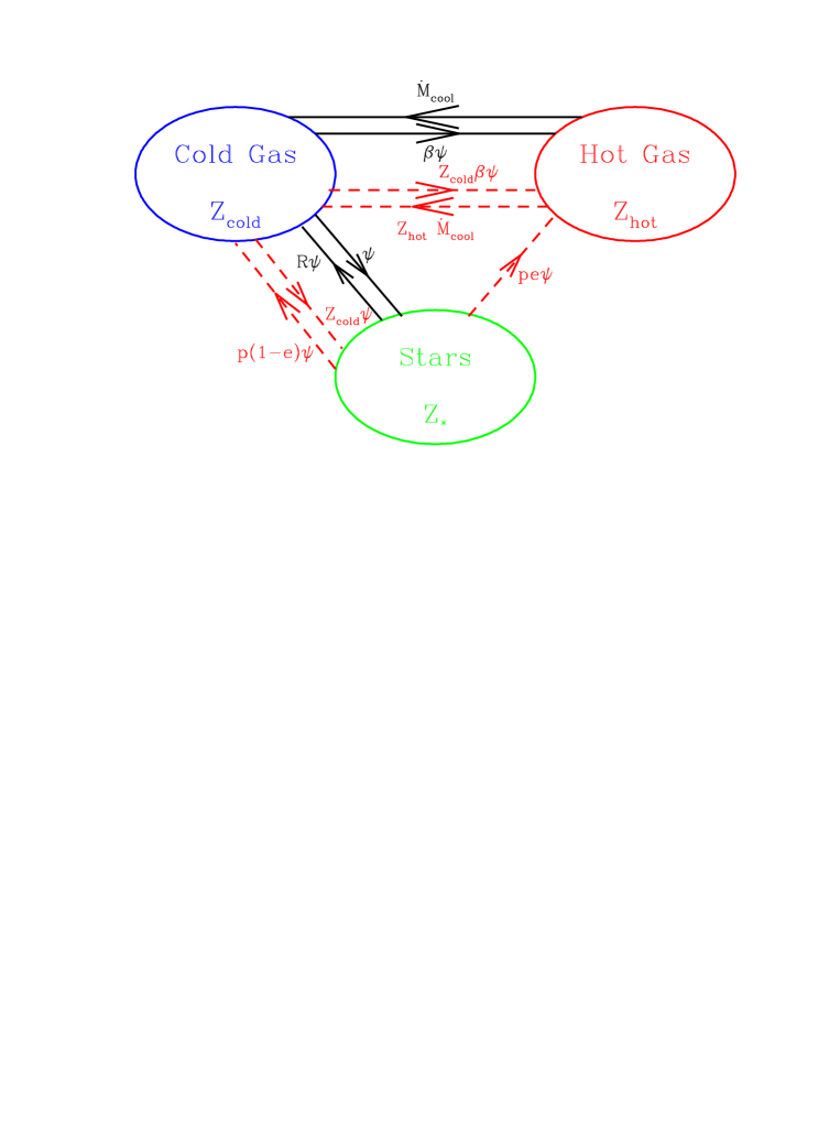
Figure 3: A schematic diagram showing the transfer of mass and metals between stars and the hot and cold gas phases during a single timestep. The solid lines indicate the routes and rates by which mass is transferred between the three reservoirs, while the dashed lines refer only to the exchange of metals. The instantaneous rate of star formation is $\psi$ and the cooling rate is $\dot{M}_{\rm cool}$. The metallicities of the cold gas, stars and hot halo gas are $Z_{\rm cold}$, $Z_{*}$ and $Z_{\rm hot}$ respectively. The yield of the assumed IMF is $p$ and the parameters $\beta$ and $e$ describe the effect of SN feedback and the direct ejection of SN metals into the hot halo gas.

4.2 Star Formation in Disks

We now turn to the important process of star formation within disks. Star formation not only converts cold gas into luminous stars, but it also affects the physical state of the surrounding gas, as SNe and young stars inject energy and metals back into the ISM. The energy that is released can be sufficient to drive gas and metals out of the galactic disk in the form of a hot wind. The removal of material from the disk acts as a feedback process which regulates the star formation rate. Also, the injected metals enrich both the cold star-forming gas and the surrounding diffuse hot halo gas. Enrichment of the halo gas decreases the cooling time defined in (4.12), allowing more gas to cool at late times, while stellar enrichment affects the colour and luminosity of the stellar populations. Early semi-analytic models were unable to include these effects accurately, as stellar population synthesis models with a wide range of metallicities were not available. Now that such models are widely available, simple chemical enrichment models have been included in several semi-analytic models, e.g. Kauffmann ([1996]), Kauffmann & Charlot([1998a]), Guiderdoni et al. ([1998]), and Somerville & Primack ([1999]).

4.2.1 Chemical Enrichment and Feedback

Our basic model of star formation assumes that stars are formed in the disk at a rate directly proportional to the mass of cold gas. Thus, the instantaneous star formation rate, $\psi$, is given by

$$\psi=M_{\rm cold}/\tau_{\star},$$ (4.13)

where the star formation timescale is $\tau_{\star}$. To model the feedback effects of energy input from young stars and SNe into the gas, we assume that cold gas is reheated and ejected from the disk at a rate

$$\dot{M}_{\rm eject}=\beta\psi.$$ (4.14)

In general, both $\tau_{\star}$ and $\beta$ are functions of the properties of the surrounding galaxy and halo. We will return later (Section 4.2.2) to the way in which we model these dependencies.

The processes of gas cooling from the reservoir of hot halo gas and accreting onto the disk, star formation from the cold gas, and the reheating and ejection of gas all occur simultaneously. For each halo, we estimate the rate at which gas cools and is accreted by the central galaxy by computing the cooling radius, as described in Section 4.1.2, at each discrete timestep at which the halo merger tree is stored. Within one of these discrete steps we approximate the cooling rate as a constant, $\dot{M}_{\rm cool}$, and use a simple instantaneous recycling approximation to model star formation, feedback and chemical enrichment ([1980]). Note that for satellite galaxies $\dot{M}_{\rm cool}=0$, as their hot gas is assumed to be stripped. Fig. 3 depicts the various channels by which mass and metals are transferred between the three phases. Note that we always compute $\dot{M}_{\rm cool}$ from the initial density profile of the hot gas and so we are implicitly assuming that gas reheated by SNe plays no role until it is incorporated into a new halo as a result of a merger. Under the instantaneous recycling approximation, the rate of flow down each channel is simply proportional to the instantaneous star formation rate, $\psi$, or the cooling rate, $\dot{M}_{\rm cool}$. The labels in Fig. 3 give the rates in terms of these quantities. The solid lines refer to total rates and the dashed lines to the metal component. Note that we have allowed for the possibility that some fraction of the metals produced by stars may be directly transferred to the hot halo gas, but we have neglected the corresponding transfer of mass. This is a good approximation, since the directly ejected material would be very metal rich and the mass transferred by this route will always be small compared to that transferred by reheating of the cold gas by SN feedback.

In Fig. 3 and below, $p$ denotes the yield (the fraction of mass converted into stars that is returned to the ISM in the form of metals), $R$ the fraction of mass recycled by stars (winds and SNe), $e$ the fraction of newly produced metals ejected directly from the stellar disk to the hot gas phase, $Z_{\rm cold}$ the metallicity of the cold gas, and $\beta$ the efficiency of stellar feedback. Each of the arrows in Fig. 3 gives rise to a term in the following differential equations that describe the evolution of the mass and metal content of the three reservoirs:

$$\dot{M}_{\star{\hphantom{col}}} = (1-R)\psi$$ (4.15)

$$\dot{M}_{\rm hot{\hphantom{l}}} = -\dot{M}_{\rm cool}+\beta\psi$$ (4.16)

$$\dot{M}_{\rm cold}^{\hphantom{Z}} = \dot{M}_{\rm cool}-(1-R+\beta)\psi$$ (4.17)

$$\dot{M}_{\star{\hphantom{olj}}}^{Z} = (1-R)Z_{\rm cold}\psi$$ (4.18)

$$\dot{M}_{\rm hot{\hphantom{l}}}^{Z} = -\dot{M}_{\rm cool}Z_{\rm hot}+(pe+\beta Z_{\rm cold})\psi$$ (4.19)

$$\dot{M}_{\rm cold}^{Z} = \dot{M}_{\rm cool}Z_{\rm hot}$$ (4.20)

$$+ (p(1-e)-(1+\beta-R)Z_{\rm cold})\psi,$$

where $Z_{\rm cold}=M_{\rm cold}^{Z}/M_{\rm cold}$ and $Z_{\rm hot}=M_{\rm hot}^{Z}/M_{\rm hot}$. The values of $R$ and $p$ in these equations are related to the IMF, as discussed in Section 5.2.

We assume that over one timestep the cooling rate, $\dot{M}_{\rm cool}$, and the metallicity of the hot gas, $Z_{\rm hot}$, can be taken to be constant. This set of first-order, coupled differential equations can be straightforwardly solved to give the change in mass and metal content of cold gas, hot gas and stars since the start of the timestep (Appendix B). The model is quite flexible: its behaviour is determined by specifying how the functions $\tau_{\star}$, $\beta$ and $e$ depend on the properties of the galaxy and its surrounding halo. We note that compared to the simple, “closed-box” chemical enrichment model, the yield is modified by the metal ejection and feedback to produce an effective yield $p_{\rm eff}=(1-e)p/(1-R+\beta)$ (equation 2.50), which is therefore a function of the potential-well depth of the galaxy. The evolution of the stellar metallicity differs from the closed-box model because it is affected by both the ejection of reheated gas and the accretion of cold gas and associated metals.

4.2.2 Star Formation Law and Feedback Parameterization

In our previous work (e.g. [1994]), we specified the star formation timescale and feedback efficiency in terms of the circular velocity of the halo in which each galaxy formed, $V_{\rm H}$. T he relations we adopted were

$$\tau_{\star}=\tau_{\star}^{0\prime}\,(V_{\rm H}/300\,{\rm km\,s^{-1}})^{\alpha_{\star}^{\prime}}$$ (4.21)

and

$$\beta=(V_{\rm H}/V_{\rm hot}^{\prime})^{-\alpha_{\rm hot}^{\prime}}.$$ (4.22)

The parameter $\tau_{\star}^{0\prime}$, we treated as a free parameter, while the other three parameters, $\alpha_{\star}^{\prime}$, $V_{\rm hot}^{\prime}$ and $\alpha_{\rm hot}^{\prime}$, we constrained by comparing our models to the numerical simulations of galaxy formation of Navarro & White ([1993]). These simulations had only one free parameter, the fraction of SN energy injected as kinetic energy into the interstellar medium. In order to suppress the formation of low luminosity galaxies, and thus produce a galaxy luminosity function with a reasonably shallow faint end slope, as observed, we adopted a fiducial model with very strong feedback for low circular velocity halos, which we obtained by setting the parameter values $\alpha_{\star}^{\prime}=-1.5$, $V_{\rm hot}^{\prime}=140\,{\rm km\,s^{-1}}$ and $\alpha_{\rm hot}^{\prime}=5.5$.

The more detailed modelling that we now perform of the structure of our model galaxies allows us to specify the star formation timescale and feedback efficiency more naturally in terms of the properties of the galaxy disk, namely its circular velocity, $V_{\rm disk}$, and dynamical time $\tau_{\rm disk}\equiv r_{\rm disk}/V_{\rm disk}$. $V_{\rm disk}$ and $r_{\rm disk}$ are both taken at the disk half-mass radius. The relations that we adopt are

$$\tau_{\star}=\epsilon_{\star}^{-1}\,\tau_{\rm disk}\,(V_{\rm disk}/200\,{\rm km\,s^{-1}})^{\alpha_{\star}}$$ (4.23)

and

$$\beta=(V_{\rm disk}/V_{\rm hot})^{-\alpha_{\rm hot}},$$ (4.24)

where $\epsilon_{\star}$, $\alpha_{\star}$ and $\alpha_{\rm hot}$ are dimensionless parameters, and the parameter, $V_{\rm hot}$, has the dimensions of velocity. If $\alpha_{\star}=0$, then our star formation law, (4.23), simply gives a star formation timescale proportional to the galaxy dynamical time, broadly consistent with the observational data compiled by Kennicutt ([1998]). The inclusion of the velocity dependent term allows us to explore models that have a similar dependence on velocity as our previous, quite successful, model which had $\alpha_{\star}^{\prime}=-1.5$ in (4.21). It should be noted that because the cold gas reservoir is depleted both by the formation of stars and by reheating due to SN feedback, the timescale on which the reservoir is depleted (in the absence of any further gas cooling) is shorter than $\tau_{\star}$. In Appendix B, where the analytic solutions of (4.15) to (4.20) are discussed, it is shown that this timescale, which in turn determines the effective star formation timescale, is given by $\tau_{\rm eff}=\tau_{\star}/(1-R+\beta)$. The feedback equation is the same as we used previously, but now expressed in terms of the galaxy circular velocity rather than the halo circular velocity. This is physically more realistic as it is the depth of the potential at the point where the stars are forming which is most relevant. To constrain these four parameters we now prefer to take a more empirical approach and use a wider range of observational data, rather than to fix the parameters to emulate one particular set of numerical simulations of galaxy formation, as we did before.

4.3 Spheroid Formation

In our model, the primary route by which bright elliptical galaxies and the bulge components of spiral galaxies form is through galaxy mergers. When dark matter halos merge, we assume that the most massive galaxy automatically becomes the central galaxy in the new halo, while all the other galaxies become satellite galaxies orbiting within the dark matter halo. The orbits of these satellite galaxies will gradually decay as energy and angular momentum are lost via dynamical friction to the halo material. Thus, eventually, the satellite galaxies spiral in and merge with the central galaxy. We now describe how we estimate the times at which such galaxy-galaxy mergers occur and what they produce.

4.3.1 Dynamical Friction

When a new halo forms, we assume that each satellite galaxy enters the halo on a random orbit. The most massive pre-existing galaxy on the other hand is assumed to become the central galaxy in the new halo, where it will act as the focus for any gas that may cool within the new halo. The time for a satellite’s orbit to decay due to the effects of dynamical friction depends on the initial energy and angular momentum of the orbit. Lacey & Cole ([1993]) estimated the time for an orbit to decay in an isothermal halo, based on the standard Chandrasekhar formula for the dynamical friction. Their formula (B4) can be written in the form,

$$\tau_{\rm mrg}=f_{\rm df}\,\Theta_{\rm orbit}\,\tau_{\rm dyn}\,\frac{0.3722}{\ln(\Lambda_{\rm Coulomb})}\frac{M_{\rm H}}{M_{\rm sat}}.$$ (4.25)

Here, $M_{\rm H}$ is the mass of the halo in which the satellite orbits, and we take $M_{\rm sat}$ to be the mass of the satellite galaxy including  the mass of the dark matter halo in which it formed ([1995a]). Note that we deliberately count the mass of the satellite’s halo in the definition of both $M_{\rm sat}$ and $M_{\rm H}$. The Coulomb logarithm, we take to be $\ln(\Lambda_{\rm Coulomb})=\ln(M_{\rm H}/M_{\rm sat})$. The dynamical time of the new halo is $\tau_{\rm dyn}\equiv\pi{r_{\rm vir}}/V_{\rm H}$, defined equivalently as either the half period of a circular orbit at the virial radius, or as $(G\rho_{\rm vir})^{-1/2}$, where $\rho_{\rm vir}$ is the mean density within the virial radius, or, for an isothermal sphere, as the full orbital period of a circular orbit at the half-mass radius.

The dependence of this merger timescale, $\tau_{\rm mrg}$, on the orbital parameters is contained in the factor $\Theta_{\rm orbit}$, defined as,

$$\Theta_{\rm orbit}=[J/J_{\rm c}(E)]^{0.78}[r_{\rm c}(E)/{r_{\rm vir}}]^{2},$$ (4.26)

where $E$ and $J$ are the initial energy and angular momentum of the satellite’s orbit, and $r_{\rm c}(E)$ and $J_{\rm c}(E)$ are the radius and angular momentum of a circular orbit with the same energy as that of the satellite. The power-law dependence on the circularity, $J/J_{\rm c}(E)$, is an accurate fit to the result of numerical integration of the orbit-averaged equations describing the effect of dynamical fiction in the range $0.01<J/J_{\rm c}(E)<1$ ([1993]). The distribution of initial orbital parameters of infalling satellites in cosmological N-body simulations has been studied by Tormen ([1997]). We find from his results that the distribution of $\Theta_{\rm orbit}$ is well modelled by a log normal with $\langle\log_{10}\Theta_{\rm orbit}\rangle=-0.14$ and dispersion $\langle(\log_{10}\Theta_{\rm orbit}-\langle\log_{10}\Theta_{\rm orbit}\rangle)^{2}\rangle^{1/2}=0.26$.

The merger timescale computed in this manner is based on several approximations, e.g. treating the satellite as a point mass with mass equal to the sum of the galaxy mass plus that of its original dark matter halo. We therefore allow ourselves some freedom by inserting the dimensionless parameter $f_{\rm df}$, which is greater than unity if the infalling satellite’s halo is efficiently stripped off early on. We note that recent analytical and numerical investigations by van den Bosch et al. ([1999]) and Colpi, Mayer & Governato ([1999]) suggest a weaker dependence of the merger timescale on the orbital circularity, with the exponent 0.78 in equation (4.26) being replaced by a value of 0.4 or 0.5, but these results were also derived using a somewhat different halo density profile from the singular isothermal sphere assumed by Lacey & Cole ([1993]). In this work we have retained the model defined by equations (4.25) and (4.26), but we note that it may soon be possible to have a fully specified and calibrated model for dynamical friction-driven mergers.

The procedure for determining the fate of satellite galaxies within dark matter halos is straightforward. When a new halo forms, each of the satellite galaxies that it contains is assigned a random value of $\Theta_{\rm orbit}$ according to the log-normal distribution described above. Then, for each satellite, we compute $\tau_{\rm mrg}$ from equation (4.25). The satellite is assumed to merge with the central galaxy after this time interval has elapsed, provided this occurs during the lifetime of the halo, i.e. before the halo has merged to become part of a much larger system. Satellites that do not merge are assigned a new random value of $\Theta_{\rm orbit}$ when the halo in which they reside is incorporated into a new, more massive halo.

4.3.2 Galaxy Mergers and Bursts

Our method for modelling galaxy mergers produces, at each timestep, a list of satellite galaxies which merge with the central galaxy in each halo. If our grid of timesteps were sufficiently fine, then these lists would always contain just one or zero satellite galaxies, but in practice there is often one large satellite and several smaller satellites merging with the central galaxy at a single timestep. We deal with this by ranking the merging satellites by mass and then, starting with the most massive one, merge them sequentially with the central galaxy.

The outcome of each merger depends on the ratio of the mass of the merging satellite, $M_{\rm sat}$, to that of the central galaxy, $M_{\rm cen}$, and has been studied recently by Walker, Mihos & Hernquist ([1996]) and Barnes ([1998]), using numerical simulations. As a simplified description of the outcome of these mergers, we adopt the prescription used in Kauffmann et al. ([1993]) and Baugh et al. ([1996a]):

• If the mass ratio of merging galaxies, defined in terms of stars and cold gas only, is $M_{\rm sat}/M_{\rm cen}\geq f_{\rm ellip}$, then the merger is said to be “violent” or “major”, and a single bulge or elliptical galaxy is produced. Any gas present in the disks of the merging galaxies is converted into stars in a burst. We use the standard star formation and feedback rules, but now based on the circular velocity and dynamical time of the spheroid that is formed rather than the disk, and with a very much shorter timescale, similar to the dynamical timescale of the spheroid.

• Alternatively, if $M_{\rm sat}/M_{\rm cen}<f_{\rm ellip}$, then the merger is classed as “minor”, and, unless explicity stated otherwise, the stars of the accreted satellite are added to the bulge of the central galaxy, while any accreted gas is added to the main gas disk without changing the disk’s specific angular momentum.

The merger simulations mentioned above have not been run for a wide enough range of initial conditions to determine $f_{\rm ellip}$ exactly, but suggest a value in the range $0.3\la f_{\rm ellip}\la 1$. The way in which we calculate the size of the spheroid which forms from a merger is described in Section 4.4.2. In the case of minor mergers, we also have the option of adding the accreted stars to the disk of the central galaxy. If we do this, we assume that the specific angular momentum of the disk is unchanged by the accretion.

4.3.3 Disk Instabilities

An issue we have not yet addressed is whether the disks in our model galaxies are dynamically stable. In particular, strongly self-gravitating disks are likely to be unstable to the formation of a bar (e.g. Binney & Tremaine [1987], §6; Efstathiou, Lake & Negroponte [1982]; Christodoulou, Shlosman & Tohline [1995]; Sellwood [1999]; Syer, Mao & Mo [1999]). Recently, the incidence of unstable disks has been considered in the context of the hierarchical formation of galaxies by Mo, Mao & White ([1998a]). Our disk model is similar to theirs, except that we explicitly follow the formation and structure of a bulge component and, more importantly, we follow the complete merging history of both the bulge and the disk. The stability criterion considered by Mo, Mao & White ([1998a]) is based on the quantity:

$$\epsilon_{\rm m}\equiv\frac{V_{\rm max}}{(GM_{\rm disk}/r_{\rm disk})^{1/2}}.$$ (4.27)

According to Efstathiou, Lake & Negroponte ([1982]), for disks to be stable requires $\epsilon_{\rm m}\ga 1.1$. In the original formulation, $V_{\rm max}$ was the rotation velocity at the maximum of the rotation curve, but in our models we use instead the circular velocity at the disk half-mass radius.

We have an option in our code to include the effect of such disk instabilities on galaxy evolution. In that case, we check the criterion (4.27) for each galaxy disk at each timestep. If at any point a disk is unstable according to this condition, we assume that the instability results in the stellar disk evolving into a bar and then into a spheroid ([1990, 1999]). We also assume that bar instability causes any gas present in the disk to undergo a burst of star formation subject to our standard feedback prescription.

We do not include the effects of disk instabilities in our reference model. We briefly present the effect it has on the distribution of disk scalelengths and the morphological mix of galaxies in Sections 7.3 and 7.4, but we postpone to a future paper a more detailed exploration of their consequences.

4.4 Galaxy Sizes

The two basic principles upon which we base our estimates of galaxy sizes are:

• the size of a disk is determined by centrifugal equilibrium and conservation of angular momentum

and

• the size of a stellar spheroidal remnant produced by mergers or disk instability is determined by virial equilibrium and energy conservation.

The application of these simple principles is complicated by the gravitational interaction of the galaxy disk, spheroid and surrounding dark matter halo. Because of this, to determine either the disk or bulge radius, we must solve for the simultaneous dynamical equilibrium of all three components. We use the following approach:

• The disk is assumed to have an exponential surface density profile, with half-mass radius $r_{\rm disk}$.

• The spheroid is assumed to follow an $r^{1/4}$ law in projection, with half-mass radius (in 3D) $r_{\rm bulge}$.

• The dark halo has a specified initial density profile (NFW in the standard case), but this is spherically deformed in response to the gravity of the disk and spheroid.

• The mass distribution in the halo and the lengthscales of the disk and bulge are assumed to adjust adiabatically in response to each other: for the disk, we assume that the total angular momentum is conserved; for the halo, we assume that $rV_{\rm c}(r)$ is conserved for each spherical shell; for the spheroid, we assume that $rV_{\rm c}(r)$ is conserved at $r_{\rm bulge}$.

The task is then to solve for $r_{\rm disk}$, $r_{\rm bulge}$ and the deformed halo profile in dynamical equilibrium, subject to these constraints. The method is described in detail in Appendix C. This adiabatic invariance method for calculating the response of a halo or spheroid to the disk was originally developed and applied by Barnes & White ([1984]), Blumenthal et al. ([1986]) and Ryden & Gunn ([1987]).

4.4.1 Disk Sizes

As already stated, the size of a disk is basically determined by the angular momentum of the halo gas which cools to form it. Many previous papers have used a version of the following argument: if the dark halo and the gas it contains are modelled as a singular isothermal sphere ($\rho\propto r^{-2}$), then, from the results of Section 3.2.3 and Appendix A, the mean specific angular momentum of the gas which cools is $j_{\rm cool}=\frac{\pi}{8}\,r_{\rm cool}V^{\rm gas}_{\rm rot}=\sqrt{2}\lambda_{\rm H}r_{\rm cool}V_{\rm H}$. On the other hand, if the self-gravity of the disk is also neglected, it rotates at constant circular velocity $V_{\rm H}$, and so has mean specific angular momentum $j_{\rm disk}=2h_{D}V_{\rm H}$, for an exponential disk with scalelength $h_{D}$. Equating $j_{\rm cool}$ and $j_{\rm disk}$ gives $r_{\rm disk}=1.68h_{D}=1.19\lambda_{\rm H}r_{\rm cool}$. This simple relation was originally derived by Fall ([1983]). It was used to calculate disk sizes in galaxy formation models (with a fixed $\lambda_{\rm H}$) by Lacey et al. ([1993]), Kauffmann & Charlot ([1994]), Kauffmann ([1996]) and Somerville & Primack ([1999]). In this paper, we improve on this simple calculation by including (a) non-isothermal halo profiles for the dark matter and gas; (b) an initial distribution of $\lambda_{\rm H}$; (c) disk self-gravity and (d) gravity of the halo and spheroid, and their contraction in response to the disk. Most of these improvements were also included in the work on disk sizes by Mo, Mao & White ([1998a]), using similar techniques to those used here. However, their work did not include a physical model for galaxy formation, so that they were forced to treat the disk-to-halo mass ratio, the disk-to-halo angular momentum ratio, and the disk $M/L$ ratio as free parameters. If for a given halo we adopt the same disk angular momentum and mass, then our model produces disk scalesizes that agree very accurately with the Mo, Mao & White model.

4.4.2 Sizes of Spheroids Formed by Mergers

Spheroids can form either in major mergers (when any pre-existing disks are destroyed) or in minor mergers (when the disk of the larger galaxy survives). To estimate the size of the spheroid formed, we assume that the merging components spiral together under the action of dynamical friction until their separation equals the sum of their half-mass radii. At this point, we assume that the systems merge together, and we use energy conservation and the virial theorem to compute the size of the remnant. These considerations lead to:

$$\frac{(M_{1}+M_{2})^{2}}{r_{\rm new}}=\frac{M_{1}^{2}}{r_{1}}+\frac{M_{2}^{2}}{r_{2}}+\frac{f_{\rm orbit}}{c}\frac{M_{1}M_{2}}{r_{1}+r_{2}},$$ (4.28)

which relates the half-mass radius of the remnant, $r_{\rm new}$, to the masses, $M_{1}$ and $M_{2}$, and half-mass radii, $r_{1}$ and $r_{2}$, of the merging components. Defining $M_{1}\geq M_{2}$, $M_{1}$ is the total galaxy mass for a major merger and the bulge mass for a minor merger, while $M_{2}$ is the total galaxy mass for a major merger and the total stellar mass of galaxy 2 for a minor merger. The masses $M_{1}$ and $M_{2}$ include contributions from the respective dark matter halos, which are taken to be twice the halo mass within the half-mass radii $r_{1}$ or $r_{2}$.

The form factor, $c$, and the constant, $f_{\rm orbit}$, are related to the gravitational self-binding energy of each galaxy,

$$E_{\rm bind}=-c\,\frac{{\rm G}M^{2}}{r}$$ (4.29)

and their mutual orbital energy,

$$E_{\rm orbit}=-\frac{f_{\rm orbit}}{2}\,\frac{{\rm G}M_{1}M_{2}}{r_{1}+r_{2}}$$ (4.30)

at the point at which the merger occurs. The value of $c$ depends weakly on the density profile of the galaxy; $c=0.49$ for an exponential disk and $c=0.45$ for an $r^{1/4}$-law spheroid. For simplicity, we adopt $c=0.5$. For the orbital energy, we adopt $f_{\rm orbit}=1.0$, which corresponds to the orbital energy of two point masses in a circular orbit with separation $r_{1}+r_{2}$. These assumptions lead to the result that, for a merger of two identical, equal mass galaxies, the half-mass radius of the remnant increases by a factor $r_{\rm new}/r_{1}=4/3$, which agrees reasonably well with the factor of $1.42$ found in the simulated galaxy mergers of Barnes ([1992]).

Having solved equation (4.28) for $r_{\rm bulge}=r_{\rm new}$, we then adiabatically adjust the spheroid, disk (if any) and halo to find the new dynamical equilibrium, as described in Appendix C. Typically, this leads to little change in $r_{\rm bulge}$, showing that our treatment of the dark matter during the merger is approximately self-consistent.

4.4.3 Sizes of Spheroids formed by Disk Instabilities

As mentioned in the previous section, our code has an option to form spheroids through bar instabilities in disks. In this case, we compute the size of the resulting spheroid using virial equilibrium and energy conservation in much the same way as for the spheroids produced by mergers. If the mass of the unstable disk is $M_{\rm disk}$, the mass of any pre-existing central stellar bulge is $M_{\rm bulge}$, and their respective half-mass radii are $r_{\rm disk}$ and $r_{\rm bulge}$, then we calculate the final bulge half-mass radius, $r_{\rm new}$, from the relation

$$\frac{c_{\rm B}(M_{\rm disk}+M_{\rm bulge})^{2}}{r_{\rm new}} = \frac{c_{\rm B}M_{\rm bulge}^{2}}{r_{\rm bulge}}+\frac{c_{\rm D}M_{\rm disk}^{2}}{r_{\rm disk}}$$ (4.31)

$$+ f_{\rm int}\frac{M_{\rm bulge}M_{\rm disk}}{r_{\rm bulge}+r_{\rm disk}}.$$

Here we adopt $c_{\rm D}=0.49$ and $c_{\rm B}=0.45$, the form factors appropriate for an exponential disk and $r^{1/4}$-law spheroid respectively (see (4.29)). The last term represents the gravitational interaction energy of the disk and bulge which is reasonably well approximated for a range of $r_{\rm bulge}/r_{\rm disk}$ by this form with $f_{\rm int}=2.0$. After we have calculated the new spheroid radius $r_{\rm new}$ from equation (4.31), we adiabatically adjust the spheroid and halo to a new dynamical equilibrium, as for the case of a spheroid formed by a merger.

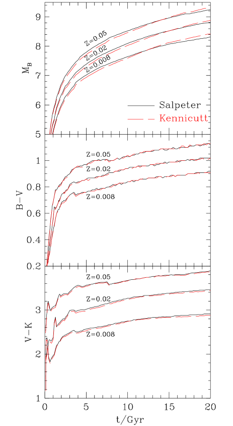
Figure 4: The evolution of the B-band luminosity and the $B$–$V$ and $V$–$K$ colours for a single age stellar population. The solid lines show results for a stellar population with a Salpeter IMF for three different metallicities. The middle curves are for solar metallicity, $Z=0.02$, and the lower and upper curves for $Z=0.008$ and $0.05$ respectively. The absolute magnitudes are normalized to $1M_{\odot}$ of stars. The corresponding dashed curves show results assuming the Kennicutt IMF. In this case, the luminosities in each band have been reduced by a factor of $1.69$ to make the solar metallicity curves for the two IMFs cross at an age of $t=15$Gyr.

5 Galaxy Luminosities and Spectra

The aspects of the model described so far enable us to follow the star formation history, chemical enrichment and size evolution of each galaxy. In order to convert this information into observable properties, we must model the spectrophotometric properties of the stars that are formed, and the effects of dust and ionized gas within each galaxy on the emerging integrated galaxy spectrum. The models we adopt for each of these processes are outlined below.

5.1 Stellar Population Synthesis

The technique of stellar population synthesis, pioneered by Tinsley ([1972, 1980]) and developed by Guiderdoni & Rocca-Volmerange ([1987]), Bruzual & Charlot ([1993]), Bressan, Chiosi & Fagotto ([1994]) and others, enables the observable properties of a stellar population to be computed given an assumption about the stellar Initial Mass Function (IMF) and the star formation history. The latest models of Bruzual & Charlot ([2000, in preparation]) provide the spectral energy distribution (SED), $l_{\lambda}(t,Z)$, of a single population of stars formed at the same time with the same metallicity, as a function of both age, $t$, and metallicity, $Z$. These can be convolved with the star formation history of a galaxy to yield its SED:

$$L_{\lambda}(t)=\int_{0}^{t}l_{\lambda}(t-t^{\prime},Z(t^{\prime}))\ \psi(t^{\prime})\ dt^{\prime},$$ (5.32)

where $Z(t^{\prime})$ is the metallicity of the stars forming at time $t^{\prime}$, and $\psi(t^{\prime})$ is the star formation rate at that time. In the case of a galaxy which formed by merging, we also sum the contributions to $L_{\lambda}$ from the different progenitor galaxies, each with their own star formation and chemical enrichment history. In performing the convolution integral, we interpolate the grid of SEDs, $l_{\lambda}(t,Z)$, provided by Bruzual & Charlot, to intermediate ages and metallicities using linear interpolation in $t$ and $\log Z$. Broad-band colours can then be extracted by integrating over these spectra weighted by the appropriate filter response function.

In our models, we always assume that the IMF is universal in time and space. Observationally, the IMF is best constrained in the solar neighbourhood. However, even here there is significant uncertainty arising mainly from ambiguity in the past star formation history. Because of this, we consider two possible choices of IMF, the form proposed by Salpeter ([1955]) and the form proposed by Kennicutt ([1983]), both of which produce reasonable agreement with the solar neighbourhood data. The Salpeter IMF has $dN/d\ln m\propto m^{-x}$ with $x=1.35$, while the Kennicutt IMF has $x=0.4$ for $m<M_{\odot}$ and $x=1.5$ for $m>M_{\odot}$. In both cases, visible stars have $0.1M_{\odot}<m<125M_{\odot}$. The Salpeter IMF has been widely used in modelling galaxy evolution because of its simplicity and the fact that it fits the observational data on high mass stars fairly well. However, there is now considerable observational evidence, as reviewed by Scalo ([1986], [1998]), that the IMF slope at low masses is flatter than the Salpeter form. The “best” IMF proposed by Scalo ([1998]), which supersedes that of Scalo ([1986]), is actually quite close to that of Kennicutt ([1983]). We therefore adopt the Kennicutt IMF as our standard choice.

We also include in our assumed IMF brown dwarfs ($m<0.1M_{\odot}$), which contribute mass but no light to the stellar population. The fraction of brown dwarfs is specified by the parameter $\Upsilon$, defined as

$$\Upsilon=\frac{({\rm mass\,in\,visible\,stars+brown\,dwarfs})}{({\rm mass\,in\,visible\,stars})}$$ (5.33)

at the time a stellar population forms, i.e. before taking account of the fraction $R$ of the mass that is returned to the ISM by recycling. Thus, by definition, $\Upsilon\geq 1$. The effect of including brown dwarfs is to reduce all stellar population luminosities by a factor $1/\Upsilon$. We will see in Section 7.7 that observational estimates of the mass-to-light ratios of stellar populations constrain viable models to have modest values of $\Upsilon$ in the range $1<\Upsilon\la 2$.

The way in which the predicted luminosity and colour of a stellar population depend on age, metallicity and choice of IMF is illustrated in Fig. 4. A number of properties which affect the behaviour of our galaxy formation models are worth noting. The overall stellar mass-to-light ratio depends significantly on the choice of IMF. This dependence has been explicitly scaled out of the curves shown in Fig. 4 by reducing all the luminosities in the Kennicutt IMF case by a factor of $\Upsilon=1.69$, so as to force the solar metallicity curves for the two IMFs to agree at $t=15$Gyr. The slope of the absolute magnitude versus time curve has some dependence on the choice of IMF. For example, as the age is reduced from $15$Gyr to around $3$Gyr, the stellar population with the Kennicutt IMF brightens more rapidly than that with the Salpeter IMF. The difference is even larger for an IMF such as the Miller-Scalo IMF ([1979]) which contains a greater fraction of stars of a few solar masses. In spite of the dependence of luminosity on the IMF, the $B$–$V$ and $V$–$K$ colours, both as a function of age and metallicity, are quite insensitive to the choice of IMF. The colours do depend strongly on metallicity, with increasing amounts of metals producing redder stellar populations. A young stellar population is very blue but rapidly reddens during its first $5$Gyr. At later times the dependence of colour on age is much weaker.

There are many approximations and assumptions involved in constructing stellar population synthesis models such as those of Bruzual & Charlot. Because of this, the accuracy of the model predictions is difficult to quantify. This issue has been addressed by Charlot, Worthey & Bressan ([1996]) by comparing model predictions from different codes and for varying sets of assumptions. Their results indicate that for the same choices of IMF and star formation history, the resulting broad-band colours can differ by a few tenths of a magnitude, and this could give rise to 20-30% uncertainties in either the inferred age or metallicity. While efforts have been made, and continue to be made, to improve these models, it should be noted that the uncertainties in the population synthesis model are sufficiently small that, for our purposes, the dominant source of uncertainty in modelling galaxy formation is, instead, the choice of IMF and its associated yield.

5.2 Yield and Recycled Fraction

There are two further quantities related to the IMF that significantly affect galaxy formation. These are the recycled fraction, $R$, and the yield, $p$. They appeared in equations (4.15) to (4.20) for the evolution of gas and star masses and metallicities. The material which goes to form massive stars is mostly released back into the ISM via stellar winds and SN explosions. The returned gas is an important source of fuel for forming further generations of stars. SN explosions also enrich the ISM with metals giving rise to subsequent generations of redder, more metal rich stars. The recycled fraction and the yield are defined so that for each mass, $\Delta M$, formed in new stars (including brown dwarfs), a mass $R\Delta M$ is returned to the ISM, and a mass $p\Delta M$ of newly synthesized metals is released. These quantities are given respectively by integrating the total ejected mass and the ejected mass in newly synthesized metals over the IMF. We recall that in a closed-box model of chemical evolution, the mean metallicity of the stars asymptotes to a value of $p/(1-R)$ as the gas is exhausted (e.g. Tinsley [1980]).

The values of $R$ and $p$ for any specific IMF can be estimated from stellar evolution theory and models of supernova explosions. We have used two different compilations of stellar evolution calculations to set these parameters: (i) Renzini & Voli’s ([1981]) for intermediate mass stars ($1<m\la 8M_{\odot}$), and Woosley & Weaver’s ([1995]) for massive stars ($m\ga 8M_{\odot}$) which produce Type II supernovae; and (ii) results from Marigo et al. ([1996]) for intermediate mass stars and from Portinari et al. ([1998]) for massive stars. The more recent calculations in (ii) include the effects of convective overshooting and quiescent mass loss. However, they rely on the supernova calculations of Woosley & Weaver. The contribution of SNII to the yield is sensitive to the assumed explosion energy (Woosley & Weaver’s cases A,B,C); we give below the corresponding range in $p$ for case (i), but Portinari et al. only calculated results for Woosley & Weaver’s case A (case C would give larger yields). Type I supernovae make only a small contribution to the net production of heavy elements, and are not included here. The results for solar metallicity are as follows: for the Kennicutt IMF, case (i) gives $R_{1}=0.42$, $p_{1}=0.013-0.023$, and case (ii) gives $R_{1}=0.44$, $p_{1}=0.022$; for the Salpeter IMF, case (i) gives $R_{1}=0.28$, $p_{1}=0.010-0.020$, and case (ii) gives $R_{1}=0.30$, $p_{1}=0.018$. These values assume that $\Upsilon=1$. If $\Upsilon>1$, the appropriate values become $p=p_{1}/\Upsilon$ and $R=R_{1}/\Upsilon$. As may be seen from these values, for a given IMF, the recycled fraction, $R$, is fairly accurately known, but the theoretically predicted yield, $p$, is uncertain by at least a factor of $2$. In our modelling, we have chosen to set $R$ according to the above estimates. However, as the yield is more uncertain, we use these estimates only as a guide for what is reasonable and instead rely on observed galaxy metallicities to constrain the value of $p$.

5.3 Extinction by Dust

Absorption of starlight by dust has a significant effect on the optical luminosities and colours of galaxies, and a large effect on the far-UV luminosities which are used as the main tracer of star formation rates at high redshift. We model the effects of dust in a physically self-consistent way, using the models of Ferrara et al. ([1999]). Ferrara et al. have calculated radiative transfer of starlight through dust, including both absorption and scattering by dust grains, for a realistic 3D distribution of stars and dust, giving the net attenuation of the galaxy luminosity as a function of wavelength and inclination angle. In their model, stars are distributed in both a bulge and a disk, and dust is distributed smoothly in a disk. The bulge follows a Jaffe ([1983]) distribution (which is very similar to an $r^{1/4}$-law) with projected half-light radius, $r_{\rm e}$. The stars and dust in the disk both have radially and vertically exponential distributions. The dust is assumed to have the same radial scalelength, $h_{R}$, as the stars, but its scaleheight, $h_{z}$, is in general different. The total dust content is parameterized by the central $V$-band optical depth, $\tau_{V0}$, defined as the extinction optical depth looking vertically through the whole disk at $r=0$. The dust properties are chosen to match observations of the extinction law and albedo of dust in either the Milky Way (MW) or Small Magellanic Cloud (SMC).

Ferrara et al. tabulate separately the attenuations of disk and bulge light, as functions of wavelength, $\lambda$, inclination, $i$, central optical depth, $\tau_{V0}$, ratio of bulge-to-disk scalelengths, $r_{\rm e}/h_{R}$, and ratio of dust-to-stellar vertical scaleheights, $h_{z,{\rm dust}}/h_{z,{\rm stars}}$. We choose a fixed value for $h_{z,{\rm dust}}/h_{z,{\rm stars}}$, and calculate $\tau_{V0}$ and $r_{\rm e}/h_{R}$ for each galaxy directly from the output of our model. We assign our galaxies random inclination angles, and then calculate the attenuation factors for the disk and bulge luminosities at the wavelengths of each of the filters (e.g. $B$, $K$) we are using by interpolating in the tables.

We calculate $\tau_{V0}$ for our model galaxies by assuming that it scales as the dust mass per unit area which, in turn, is assumed to scale with the total mass of metals per unit area in the cold gas:

$$\tau_{V0}\propto{M_{\rm dust}\over r_{\rm disk}^{2}}\propto{M_{\rm cold}Z_{\rm cold}\over r_{\rm disk}^{2}}.$$ (5.34)

The metallicity $Z_{\rm cold}$ is obtained from our chemical evolution calculation. We normalize equation (5.34) by assuming that gas with solar metallicity, $Z=0.02$, has the local ISM dust-to-gas ratio. Savage & Mathis ([1979]) find $A_{V}/N{\rm{}_{H}}=3.3\times 10^{-22}{\rm mag\,}{\rm cm}^{2}$ for the local ratio of $V$-band extinction, $A_{V}$, to hydrogen column density $N_{\rm H}$. This then implies

$$\tau_{V0}=0.043\left({M_{\rm cold}/(2\pi h_{R}^{2})\over M_{\odot}{\rm pc}^{-2}}\right)\left({Z_{\rm cold}\over 0.02}\right).$$ (5.35)

Our standard choice is to use an MW extinction curve and to assume $h_{z,{\rm dust}}/h_{z,{\rm stars}}=1$. We have investigated variations in $h_{z,{\rm dust}}/h_{z,{\rm stars}}$ over the range 0.4 to 2.5, and find that most results are very insensitive to this. Most results also do not change significantly if an SMC rather than an MW extinction curve is used. The SMC and MW extinction curves differ significantly only in the far-UV, but even here, the effects on our results are fairly small, as the net attenuation of galaxy light calculated using these radiative transfer models has a much weaker (“greyer”) dependence on wavelength than in a simple foreground screen model. Our model for dust absorption thus has essentially no significant free parameters. Results are sensitive mostly to the value of $\tau_{V0}$, which is calculated directly from our other model quantities.

Our modelling of dust extinction is a major improvement over what has been done previously in semi-analytic models, both in terms of including a realistic 3D distribution for the stars and dust, and in terms of calculating the dust optical depth in a physically self-consistent way. The first semi-analytic models to include dust were those of Lacey et al. ([1993]), using the dust and stellar population model of Guiderdoni & Rocca-Volmerange ([1987]), and Guiderdoni et al. ([1998]). They modelled the star and dust distributions as a uniform 1D slab, but calculated the dust content self-consistently from a closed-box chemical evolution model. Kauffmann et al. ([1999a]) and Somerville & Primack ([1999]) also use the 1D slab model, but instead of predicting the slab optical depth, they use a power-law relation between dust optical depth and galaxy luminosity that is estimated from observations of $z=0$ galaxies.

The main deficiencies of our current dust model are that it does not allow for clumping of the dust and stars or deal well with bursts, and that it only calculates absorption by dust, but not the spectrum of dust emission. However, Silva et al. ([1998]) have developed a more sophisticated dust model which includes both clumped and smooth components of the dust, deals accurately with bursts and is able to predict not only the extinction of starlight, but also the spectrum of the energy re-radiated by the dust in the far infra-red and sub-mm. Granato et al. ([2000]) combine this dust model with our galaxy formation model to predict galaxy luminosity functions in the far infra-red and sub-mm and Lacey et al. ([2000a]) investigate the high redshift behaviour and predict number counts and integrated radiation backgrounds.

5.4 Emission line Modelling

We model the emission lines from photo-ionized gas in our galaxies by calculating the luminosity in Lyman continuum photons from the stellar population using the Bruzual & Charlot models, and combining this with HII region models to calculate line luminosities and equivalent widths. We have calculated results for important lines used as star formation indicators, such as H$\alpha$ and OII. This is described in detail in a separate paper ([2000b]).

6 Methodolgy

6.1 Model Parameters

The complete hierarchical model of galaxy formation described in the previous section contains a significant number of parameters. However, relatively few should be considered as free parameters. These fall into three distinct categories: numerical parameters, parameters of the cosmological model and, finally, parameters related directly to our modelling of the physics of galaxy formation.

The parameters that fall in the first set include the mass resolution, $M_{\rm res}$, the number of timesteps in the merger tree, $N_{\rm steps}$ and the starting redshift, $z_{\rm start}$. These do not represent freedoms of the model, and we must simply choose values such that the quantities of interest have converged and are insensitive to further improvements. Also, there are options such as adopting singular isothermal spheres to describe the dark matter and gas density profiles, or varying the distribution of halo spin parameters, which are not to be viewed as viable alternatives. Instead, we have included them simply in order to be able to vary our assumptions so as to gain insight into why the model behaves in a particular way. In these examples, any viable model should employ the options that are consistent with results of the high-resolution simulations that we are trying to emulate.

The second set are parameters that specify the background cosmological model. These include the density parameter, $\Omega_{0}$; the cosmological constant, $\Lambda_{0}$; the Hubble constant, $h$; the baryon density, $\Omega_{\rm b}$; and the shape and amplitude of the linear theory mass power spectrum, $P(k)$. In principle, each of these can be determined from observations that do not depend on galaxy properties. For example, most of these cosmological parameters are likely to be determined accurately from microwave background anisotropy measurements to be carried out by the MAP and Planck satellite missions (e.g. [1997]). Alternatively, the power spectrum amplitude, $\sigma_{8}$, may be fixed by reference to the abundance of galaxy clusters, while the baryon density may be constrained by models of primordial nucleosynthesis and the observed abundance of the light elements, like deuterium, at low and high redshift. Our general approach is to set these parameters according to such external constraints. However, some properties of the galaxy formation models are particularly sensitive to the baryon density, $\Omega_{\rm b}$, and to the normalization, $\sigma_{8}$. For this reason, we sometimes allow some variation of these parameters around the values otherwise indicated by the external observational constraints.

The final set of parameters are those with which we directly characterize our physical model of galaxy formation. Firstly, there is the IMF and its associated yield of metals, $p$, and the fraction, $R$, of stellar mass that is liberated in stellar winds and SNe. In principle, $p$ and $R$ are fixed by the choice of IMF, but, in practice, although $R$ is quite well constrained, $p$ is quite uncertain. Secondly, we have the parameters, $\epsilon_{\star}$, $\alpha_{\star}$, $V_{\rm hot}$ and $\alpha_{\rm hot}$ in the star formation and feedback laws. Then, there is the parameter, $e$, the fraction of the metals produced in SNe which escape directly to the hot diffuse halo gas. Also, we require the vertical scale-height of dust relative to that of the disk stars (although our results are very insensitive to this parameter). Finally, there are the parameters $f_{\rm df}$ and $f_{\rm ellip}$, which modulate the frequency of galaxy-galaxy mergers and determine when a merger results in the formation of a spheroid. Although the number of model parameters is not small, we shall see that the resulting freedoms of the model are still quite limited and that only a small subset of observed properties of low redshift galaxies are needed to constrain a model fully.

6.2 Model Output

The output of our code is a list of the galaxies that form in each simulated halo at one or more redshifts. For each galaxy the output lists: a flag which indicates whether the galaxy is the central galaxy of the halo in which it is contained or a satellite galaxy; the mass of cold gas in the disk; the mass of stars in the disk and bulge; the luminosities in any chosen band of the stars in the disk and bulge; selected emission line luminosities and equivalent widths; the half-mass radius of the disk and bulge individually and combined; the circular velocities at the half-mass radii of the disk and bulge; the metallicity of the cold gas and also, if the galaxy is a central galaxy, the metallicity of its hot gas halo; the metallicities and age of the bulge and disk stars weighted by mass or by luminosity in any selected band; the instantaneous star formation rate in the disk; the mass and circular velocity at the virial radius of both the halo in which the galaxy was last a central galaxy and the halo in which it is contained at the chosen output redshift. The effect of dust within each galaxy on the luminosities and line strengths is computed in an additional step by assuming an inclination angle for each galaxy. Also, since we know the disk and bulge sizes, we can compute surface brightness distributions and isophotal magnitudes for each individual galaxy, assuming exponential profiles for disks and $r^{1/4}$ profiles for spheroids. Since we also know the number density of each of the halos we have simulated, it is straightforward to estimate galaxy luminosity functions and galaxy number counts (both using either total or isophotal magnitudes) or to sample our output to build up either volume-limited or magnitude-limited galaxy catalogues from which to draw galaxy samples for comparison with observational datasets. In this work we have used the halo abundance given by the Press-Schechter formalism, but it is now possible to adopt improved analytic estimates (Sheth, Mo & Tormen [2000]) which accurately match the abundance of halos found in large N-body simulations (Jenkins et al. [2000]). We have checked that switching to these more accurate formulae changes the model results far less than varying some of the galaxy formation parameters.

Once we have calculated a model, we have the ability to select from the output any particular galaxy and recompute its formation history, this time choosing to output its properties more frequently and to record its star formation and merger history. In this way we can generate the complete formation history of selected galaxies and, for each, construct their own individual merger trees. Examples of galaxy merger trees constructed in this way have been presented in Figure 9 of Baugh et al. ([1998]).

6.3 Strategy

Our adopted methodology is to select a cosmological model based on constraints from large-scale structure and then vary the galaxy formation parameters in order to match as best as possible a selection of low-redshift observational data. Since galaxy formation is undoubtedly a complex process, the simple model we have constructed cannot aspire to be a complete and full description. Thus, it is inevitable that in some cases our models will only produce a moderate level of agreement with certain observational data.

In the following section, we illustrate this process of defining the parameters of the galaxy formation model for one particular cosmology. We use this example to illustrate the way in which we apply the observational constraints and to show how the model predictions depend on each of the model parameters.

7 Observational constraints on the model and effects of varying the parameters

In the following sub-sections, we compare models constructed within a particular cosmology with a variety of statistics estimated from the observed properties of the local galaxy population. For each statistic, we illustrate how the predictions of the galaxy formation model depend on the parameters, and present one model, our reference model, which is the best compromise when measured against a full range of observational data. The observational constraints used to fix each of the main parameters of our reference model are as follows:

• $\alpha_{\rm hot}$: faint end of luminosity function and Tully-Fisher relation

• $V_{\rm hot}$: faint end of luminosity function and sizes of low luminosity spirals

• $\epsilon_{\star}$: gas fraction for $L_{\star}$ spirals

• $\alpha_{\star}$: variation of gas fraction with luminosity

• $f_{\rm ellip}$: morphological mix for $L_{\star}$ galaxies

• IMF: observations of solar neighbourhood

• $\Upsilon$: $L_{\star}$ in luminosity function

• $p$: metallicity of $L_{\star}$ ellipticals

The chosen parameters values of our reference model are listed in Table 1.

We emphasize that not all of the observational data presented in this section are used to fix model parameters - some of the data provide tests of the model, and are shown in this section to illustrate the effects of varying the parameters.

The cosmology that we have chosen in order to illustrate how observational data may be used to constrain the galaxy formation parameters is a flat, low-density cold dark matter model with a cosmological constant. The parameters that we adopt for this $\Lambda$CDM model are $\Omega_{0}=0.3$ and $\Lambda_{0}=0.7$. Such a model is currently favoured by quite a range of observational evidence. For reasonable values of the Hubble constant ($h\sim 0.7$), the shape of the mass power spectrum is in good agreement with estimates from large-scale galaxy clustering (e.g. [1990]). The value of $\Omega_{0}$ is consistent with the high baryon fraction in clusters ([1993, 1995, 1997]) and with the mild evolution in the abundance of X-ray clusters ([1998]). The joint values of $\Omega_{0}$ and $\Lambda_{0}$ are in accord with estimates from high redshift SNe ([1998, 1998, 1998]), while $\Omega_{0}+\Lambda_{0}=1$ is in agreement with the detection of the first CMB Doppler peak ([2000, 2000, 2000, 2000]). For this model, the normalization of the mass power spectrum, $\sigma_{8}$, derived from the number density of X-ray emitting galaxy clusters is consistent with that from the amplitude of CMB fluctuations (e.g. [1997]), and both are consistent with the power spectrum of the mass at $z=2.5$, inferred by Croft et al. ([1999]) and Weinberg et al. ([1999]) from analysis of the Lyman-$\alpha$ forest.

Table 1: The values of the model parameters for the reference model.

$\Omega_{0}$	$\Lambda_{0}$	$\Omega_{\rm b}$	$h$	$\Gamma$	$\sigma_{8}$	$\epsilon_{\star}$	$\alpha_{\star}$	$V_{\rm hot}$	$\alpha_{\rm hot}$	$e$	$f_{\rm ellip}$	$f_{\rm df}$	IMF	$p$	$R$	$\Upsilon$
0.3	0.7	0.02	0.7	0.19	0.93	0.005	-1.5	200.0	2.0	0.0	0.3	1.0	Kennicutt	0.02	0.31	1.38

The galaxy formation model as a whole is a complex system, with the result that the dependence of a particular statistic on a given parameter can be complicated. Thus, when one parameter is varied, the behaviour of the model certainly depends on the other constraints that have been applied. This fact, combined with the number of parameters, makes it unfeasible to present the full range of possible model behaviour. One should therefore be careful not to over-interpret the trends discussed below: since the effects of varying one parameter can depend on the values of the others, it is dangerous to assume that these trends can be used to assess the result of varying more than one parameter at a time.

As well as varying the parameters that regulate the physics of galaxy formation, we allow some variation of the parameters, $\sigma_{8}$, $h$ and $\Omega_{\rm b}$, that define the cosmological model. However, these are only allowed to vary within the ranges permitted for consistency with estimates of the abundance of rich galaxy clusters, Hubble’s constant, and primordial nucleosynthesis. Whenever we vary any of these parameters, we consistently adjust the power spectrum shape parameter, $\Gamma$, according to the fitting formula for CDM proposed by Sugiyama ([1995]):

$$\Gamma=\Omega_{0}h\,\exp\left(-\frac{\Omega_{\rm b}}{\Omega_{0}}(\sqrt{2h}+\Omega_{0})\right).$$ (7.36)

The estimated values and 1-$\sigma$ errors that we adopt for these quantities are $\sigma_{8}=0.93\pm 0.07$ ([1996]), $h=0.7\pm 0.1$ ([1998, 1998]), and $\Omega_{\rm b}h^{2}=0.0125\pm 0.0025$ ([1991]). We note that somewhat higher values of $\Omega_{\rm b}h^{2}$ are favoured by recent estimates of the D/H ratio from QSO absorption line systems ([1998, 1998]), and by models of the mean optical depth of the Lyman-$\alpha$ forest ([Rauch et al. 1997, Weinberg et al. 1997]). We discuss the consequences of increasing our adopted value of $\Omega_{\rm b}$ in Section 9.

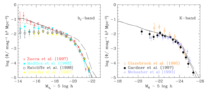
Figure 5: Comparison of the ${\rm b_{J}}$ and K-band galaxy luminosity functions in the $\Lambda$CDM reference model with a compilation of observational data. The solid line is the model including the effects of dust, with $\Upsilon$ chosen so as to obtain agreement with the observed luminosity functions at $M_{\rm b_{J}}-5\log h=-19.8$. The dashed lines show the corresponding luminosity functions before the effects of dust extinction are included. The dotted line on the left hand panel shows how the luminosity function is modified if the isophotal magnitude within an isophote of 25 ${\rm mag}/{\rm arcsec}^{2}$ is used instead of the true total magnitude. See §7.3 for details.

In a similar fashion, many of the parameters that describe the physics of galaxy formation can only plausibly be varied by modest amounts. Consider, for example, the threshold, $f_{\rm ellip}$, above which galaxy mergers are termed violent and assumed to result in the formation of an elliptical galaxy. By definition, $f_{\rm ellip}\leq 1$, and based on simulations of galaxy mergers, a reasonable lower limit is $f_{\rm ellip}\ga 0.3$ (Walker et al. [1996]; Barnes [1998]). Other parameters that are similarly constrained to lie within relatively narrow ranges are $f_{\rm df}$ and, to a lesser extent, $p$. The merger timescale coefficient, $f_{\rm df}$, should be close to unity if an infalling galaxy retains its dark matter halo throughout most of the time when dynamical friction is removing angular momentum and energy from its orbit. It could be larger than unity if the dark matter halo is efficiently stripped off at early times, but cannot plausibly be significantly smaller than unity. As described in Section 5.1, the choice of IMF quite accurately determines the recycled fraction, $R$, and also sets some constraint on the yield, $p$.

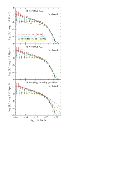
Figure 6: The effect on the ${\rm b_{J}}$-band luminosity function of varying the star formation and feedback parameters, $\alpha_{\rm hot}$ and $V_{\rm hot}$, and the assumed halo DM and hot gas density profiles. In all cases, the value of $\Upsilon$ has been fixed by requiring the model luminosity functions to agree with the observations at $M_{\rm b_{J}}-5\log h=-19.8$. a) Shows how increasing $\alpha_{\rm hot}$ suppresses the formation of low-luminosity galaxies and so controls the faint-end slope of the luminosity function. The dotted curve is for $\alpha_{\rm hot}=1$, solid for $\alpha_{\rm hot}=2$, and dashed for $\alpha_{\rm hot}=5.5$. b) Demonstrates how increasing $V_{\rm hot}$ lowers the faint end of the luminosity function. Results are shown for $V_{\rm hot}=100\,{\rm km\,s^{-1}}$ (dotted curve), $V_{\rm hot}=200\,{\rm km\,s^{-1}}$ (solid curve), and $V_{\rm hot}=300\,{\rm km\,s^{-1}}$ (dashed curve). c) Shows how the bright end of luminosity function depends on the model adopted for the density profile of the hot gas. The solid curve is our reference model which has an NFW profile for the DM and the “$\beta$-model” for the gas, with a core radius that depends on the fraction of gas that has previously cooled (see Section 4.1.1). The dotted and long-dashed curves also assume NFW profiles for the DM, but assume a fixed core radius “$\beta$-model” (dotted) or an NFW profile for the gas (long-dashed). The short-dashed line is for a singular isothermal sphere ($\rho\propto r^{-2}$) model for both gas and DM.

7.1 Galaxy Luminosity Functions

The single most important constraint on our galaxy formation models is the local galaxy luminosity function. This is one of the most fundamental properties of the galaxy population and it is also one of the best measured, at least over a restricted range of luminosities. Matching the galaxy luminosity function is a prerequisite for any realistic model of galaxy formation, because the detectability of galaxies depends directly on their luminosity. Thus, a model that fails to match the bright end of the luminosity function can lead to misleading conclusions when tested, for example, against samples selected by apparent magnitude.

Fig. 5 shows estimates of the local galaxy luminosity function in the blue optical ${\rm b_{J}}$-band and in the near infrared K-band. The ${\rm b_{J}}$-band data are taken from the APM-Stromlo galaxy redshift survey ([1992]), the ESO slice project ([1997]), the DUKST survey ([1998]) and from preliminary results from the 2dF galaxy redshift survey ([1998]). The K-band data are from Mobasher et al. ([1993]), Glazebroook et al. ([1995]) and Gardner et al. ([1997]). In both bands, there is reasonably good agreement among the various estimates at the bright end. At the faint end, however, there is considerable dispersion among the results from different surveys. In the ${\rm b_{\rm J}}$-band these differences are large compared to the statistical errors. We must, therefore, conclude that either the galaxy luminosity function differs in the different volumes surveyed, or that systematic differences in the selection characteristics of the surveys give rise to these differences.

The solid and dashed model curves shown in Fig. 5 correspond to the reference model, both with and without the inclusion of dust. In the model with dust, the vertical scaleheight of the dust distribution was taken to be the same as that of the disk stars, but varying this assumption makes very little difference to the luminosity functions. The model without dust produces a reasonable K-band luminosity function, but it gives rise to galaxies which are systematically too bright in ${\rm b_{J}}$. By contrast, the model with dust is a good fit to the bright end of both the ${\rm b_{J}}$ and K-band luminosity functions. We shall see below that the differential effect of dust, which generates greater extinction at shorter wavelengths, is important in providing a good match to the observed $B$–$K$ colour distributions. It also results in a model that comes significantly closer than our previous models to matching simultaneously the zero-point of the observed I-band Tully-Fisher relation and the bright end of the ${\rm b_{J}}$-band luminosity function, thus largely overcoming an important shortcoming of our earlier models ([1994]). The importance of the role of dust in achieving this simultaneous match has also been noted by Kauffmann et al. ([1999a]) and Somerville & Primack ([1999]). The prescription for the dust distribution assumed in Fig. 5 will be retained in all the following comparisons.

Many of the model parameters have a direct effect on the galaxy luminosity function. Typically, varying any one of them on its own causes only a minor change in the shape of the luminosity function, but can cause a significant overall shift (either left or right) in the luminosity scale. Our normalization strategy separates out these two effects by adjusting the parameter $\Upsilon$ so as to keep the amplitude of all the luminosity functions fixed at $M_{\rm b_{J}}=-19.8+5\log h$. Recall that $\Upsilon^{-1}$ is the initial stellar mass fraction in luminous stars (equation 5.33), and that the remaining fraction is assumed to be made up of non-luminous brown dwarfs. Physically, one ought to vary the net recycled fraction $R$ when adjusting $\Upsilon$, so as to keep the value $R_{1}=\Upsilon R$ constant for the luminous stars alone (§ 5.2). The reference model has $\Upsilon$ and $R$ chosen consistently to give $R_{1}=\Upsilon R=0.42$ for the Kennicutt IMF, as found in Section 5.2. To achieve this requires some iteration as the value of $\Upsilon$ is determined after the model has been run by matching a point in the B-band luminosity function. For this reason, when showing the effects of varying parameters we choose to keep $R$ constant rather than $R_{1}$.

The effect of parameter changes on the position of the luminosity function is summarized in Table 2. Here, we give the values of $\Upsilon$ required to shift each luminosity function into coincidence with the Zucca et al. ([1997]) luminosity function at $M_{\rm b_{J}}=-19.8+5\log h$. We will see in Section 7.7 that in models which have realistic stellar mass-to-light ratios, $\Upsilon\sim 1.3-2$ for the Kennicutt IMF. In a few cases, however, this normalization procedure requires $\Upsilon<1$, which is unphysical. (It corresponds approximately to removing from the IMF all of the brown dwarfs and some of the low mass visible stars, by increasing the lower mass limit above $0.1M_{\odot}$.) Nevertheless, we present these models because they help to clarify some of the trends that occur when a single parameter is varied. For the derived normalization of $\Upsilon$, the table gives other properties of the galaxy population. Several of the entries in this table are discussed further in the relevant sections below.

Table 2: The variation of the average colour, the mass-to-light ratio of the stellar populations and the zero-point of the Tully-Fisher relation with model parameters. In all cases, $\Upsilon$ is adjusted so as to match the observed $\rm b_{J}$-band luminosity function at $M_{\rm b_{J}}=-19.8+5\log h$. The first column lists the parameter that has been varied relative to the reference $\Lambda$CDM model. The second column gives the required value of $\Upsilon$. The third lists the median $B$–$K$ colour for galaxies in the range $-24.5<M_{\rm K}-5\log h<-23.5$. The following four columns list the median B- and I-band stellar mass-to-light ratios, in units of $h{\rm M_{\odot}/L_{\odot}}$, for disk and elliptical galaxies with $-20<M_{\rm B}-5\log h<-19.0$. These are compared with observed values in Section 7.7. The last two columns show the offset in magnitudes from the observed I-band Tully-Fisher relation at $V_{\rm disk}=160\,{\rm km\,s^{-1}}$, and the median ratio of the circular velocity of the disk to that at the virial radius of the halo in which it formed for galaxies with $-20<M_{\rm I}-5\log h<-18$.

Modified Parameter	$\Upsilon$	$B$–$K$	Disk: $M/L_{\rm B}$	Disk: $M/L_{\rm I}$	Elliptical: $M/L_{\rm B}$	Elliptical: $M/L_{\rm I}$	$\Delta M_{I}$	$V_{\rm disk}/V_{\rm halo}$
Reference Model	1.38	3.86	2.0	1.8	5.4	2.9	0.98	1.35
No Dust	2.30	3.60	2.1	2.4	8.7	4.9	1.48	1.41
$\alpha_{\rm hot}=1$	1.39	3.81	2.1	1.8	4.8	2.8	1.13	1.50
$\alpha_{\rm hot}=5.5$	1.1	4.01	1.4	1.2	4.3	2.3	1.02	1.02
$V_{\rm hot}=100\,{\rm km\,s^{-1}}$	1.32	4.11	2.5	2.0	6.3	3.1	1.73	1.71
$V_{\rm hot}=300\,{\rm km\,s^{-1}}$	1.15	3.56	1.2	1.2	2.5	1.8	0.75	1.20
$\alpha_{\star}=0.0$	1.28	3.96	2.0	1.7	5.4	2.8	0.83	1.27
$\alpha_{\star}=-2.5$	1.31	3.81	1.7	1.5	5.0	2.8	1.09	1.41
$\Omega_{\rm b}=0.01$	0.45	3.62	0.5	0.5	1.0	0.7	0.23	1.13
$\Omega_{\rm b}=0.04$	3.07	4.11	7.3	4.7	13.9	6.9	2.12	1.96
$h=0.6$	0.95	3.87	1.7	1.5	4.8	2.6	0.92	1.34
$h=0.8$	1.77	3.86	2.1	1.9	5.4	3.0	1.19	1.38
$\epsilon_{\star}=0.01$	1.70	3.85	2.1	1.9	7.4	3.9	1.12	1.30
$\epsilon_{\star}=0.0033$	1.13	3.90	1.8	1.5	4.5	2.5	1.03	1.40
$p=0.0075$	1.66	3.28	1.6	1.7	3.9	2.7	1.01	1.36
$p=0.03$	1.17	4.16	2.1	1.7	5.7	2.8	0.92	1.34
$R=0.19$	1.31	3.80	2.1	1.9	5.9	3.2	1.07	1.38
$R=0.49$	1.41	3.97	1.7	1.4	3.7	2.0	0.85	1.31
$\sigma_{8}=0.86$	1.43	3.82	2.0	1.7	4.2	2.5	1.03	1.34
$\sigma_{8}=1.0$	1.48	3.90	2.2	1.9	6.1	3.3	1.20	1.38
IMF: Salpeter, $R=0.28$	0.79	3.85	1.9	1.7	5.5	3.0	1.00	1.35
$f_{\rm form}=1.5$	1.27	3.82	1.9	1.6	5.1	2.8	0.93	1.42
$f_{\rm df}=0.5$	1.34	3.89	2.0	1.7	4.4	2.5	1.03	1.36
$f_{\rm df}=2.0$	1.16	3.80	1.5	1.4	4.8	2.6	0.84	1.34
$f_{\rm ellip}=0.5$	1.38	3.90	2.1	1.8	5.8	3.1	0.99	1.35
$r_{\rm core}=r_{\rm NFW}/6$	1.40	3.85	2.0	1.8	5.4	3.0	1.05	1.35
Fixed gas core radius	1.23	3.97	2.3	1.8	2.9	1.9	0.87	1.34
NFW gas traces DM	1.23	4.04	2.5	1.8	3.1	2.0	0.92	1.34
SIS gas traces DM	1.08	4.24	2.4	1.7	3.4	2.0	0.95	1.41
Unstable disks	1.50	3.91	2.1	1.9	4.7	2.8	1.11	1.28
Accretion by disk	1.40	3.89	2.3	1.9	5.5	3.0	1.12	1.38

Two parameters that strongly affect the shape of the galaxy luminosity function are $V_{\rm hot}$ and $\alpha_{\rm hot}$, the quantities that define our model of stellar feedback (equation 4.24). As can be seen in Fig. 6a, the faint-end slope of the luminosity function is very sensitive to $\alpha_{\rm hot}$, with large values producing a shallower slope. Similarly, as Fig. 6b shows, increasing $V_{\rm hot}$ also reduces the number of faint galaxies. Both these dependencies are easily understood: stronger stellar feedback makes it increasingly more difficult for luminous stars to form in low-mass halos. To match the very shallow faint-end slope seen in the data of Loveday et al. ([1992]) or Ratcliffe et al. ([1998]), requires a high value of $\alpha_{\rm hot}$, such as that adopted by Cole et al. ([1994]), who compared their models against the first of these surveys. Such a value, however, would lead to a disagreement with the data of Zucca et al. ([1997]). The differing observational estimates of the luminosity function indicate that the faint-end slope is not as robustly determined as one might wish, perhaps because it depends on the details of the survey selection criteria. We therefore do not use it as a model constraint. Instead, we will see in Section 7.2 that extreme values of $\alpha_{\rm hot}$ are disfavoured on other grounds and this leads us to favour models whose luminosity functions have quite steep faint end slopes.

The bright end of the luminosity function is sensitive to the density profile assumed for the halo gas, because this controls how much of the gas can cool. This effect is not important in low-mass halos, in which the gas temperature ${T_{\rm vir}}$ is low enough that most of the gas can cool anyway, but it becomes important in large groups and clusters, in which only the dense central regions have time to cool. Fig. 6c compares the effects of using different gas profiles. Our reference model (shown by the solid line) assumes an NFW dark halo and a $\beta$-model for the gas (equation 4.11), with a core radius that starts at $r_{\rm core}=r_{\rm NFW}/3$ and grows depending on how much gas has already cooled in progenitor halos. The model luminosity function and other properties are not sensitive to the precise value of this initial core radius. For example, if instead, we set $r_{\rm core}=r_{\rm NFW}/6$ as the initial value, then the change in the luminosity function is almost too small to be visible and the other properties listed in Table 2 also only vary slightly. In principle, constraints can be placed on the initial gas density profile from the observed X-ray emission profiles of groups and clusters, but in practice this requires complex modelling to take account of the emission associated with the central cooling flow.

Our model fits the observed bright end of the luminosity function well. It is compared in the figure to a model in which the gas core radius is kept fixed at $r_{\rm core}=r_{\rm NFW}/3$ (dotted curve), another in which both gas and dark matter have the same NFW profile (long-dashed curve), and finally to a model in which both gas and dark matter have singular isothermal sphere profiles (short-dashed curve), as has been assumed in most previous work. The latter three models produce many more high luminosity $L\ga L_{\star}$ galaxies than is observed. This difference in the assumed halo gas profiles explains most of the differences in the shape of the bright end of the luminosity function between our reference model and the models of Kauffmann et al. ([1993],[1999a]) and Somerville ([1997]), although the procedure in these papers of using the Tully-Fisher relation rather than the luminosity function as the primary observational constraint also has an effect. These authors all invoke an artificial cut-off on the circular velocity of halos in which gas is allowed to cool to form visible stars, in order to ameliorate their problems in fitting the luminosity function. We believe that our standard model for cooling is the most physically reasonable in this regard, for the reasons given in Section 4.1.1. More recently, Somerville & Primack ([1999]) have presented models with no artificial cooling cut-off which nevertheless produce a good match to the bright-end of the B-band luminosity function. In this case, this improvement is achieved partly as a result of the empirical dust model they have adopted, which has an extinction that increases with increasing galaxy luminosity. However, as dust has less effect in the K-band, they find that for some of their models, the shape of the bright-end of the K-band luminosity function remains a poor match to observations.

As was shown in Cole et al. ([1994]), the shape of the luminosity function is also influenced by the efficiency of galaxy mergers, which is controlled by $f_{\rm df}$. However, we now impose the constraint $f_{\rm df}\ga 1$, a limit suggested by numerical simulations ([1995a]), which also leads to an acceptable morphological mix in the model. With this bound, the residual variation in the shape of the luminosity function with $f_{\rm df}$ is small compared to its dependence on the feedback parameters $V_{\rm hot}$ and $\alpha_{\rm hot}$ and on the halo gas profile. Our treatment of feedback is, in fact, the main factor responsible for the overall shape of the model luminosity function at $L\la L_{\star}$, and our assumptions about cooling are the main determinant of the shape at $L\ga L_{\star}$.

7.2 The Tully-Fisher Relation

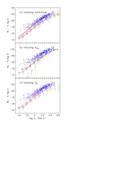
Figure 7: The dependence of the model I-band Tully-Fisher relation on a) the sample selection criteria, b) the feedback parameter, $\alpha_{\rm hot}$, and c) the baryon density, $\Omega_{\rm b}$. In each case, the model curves trace the median magnitude as a function of circular velocity, and the errorbars show the 10 and 90 percentiles of the distribution. The magnitudes are face-on values, including the effects of dust. The points show the observed distribution for a subsample of Sb-Sd galaxies selected by de Jong & Lacey ([2000]) from the Mathewson, Ford & Buchhorn([1992]) catalogue and, again, all magnitudes have been corrected to face-on values. All the curves in the top panel are for the reference model, but for different galaxy selection criteria. The dotted line is for all spiral galaxies which are the central galaxies in their halos, the dashed line for all spiral galaxies (both central and satellite), and the solid line for all star-forming spiral galaxies with gas fractions of 10% or greater (this final selection is retained in b & c). The thick solid line shows, for central galaxies, the result of using the circular velocity at the virial radius of the halo in which the galaxy formed, rather than the disk circular velocity. In b), the solid line refers to the reference model (which has $\alpha_{\rm hot}=2$), while the dashed line is for $\alpha_{\rm hot}=1$ and the dotted line for $\alpha_{\rm hot}=5.5$. In c), the solid line refers, again, to the reference model (which has $\Omega_{\rm b}=0.02$), while the dashed line is for $\Omega_{\rm b}=0.01$ and the dotted line for $\Omega_{\rm b}=0.04$.

In Fig. 7, we compare our predicted I-band Tully-Fisher (TF) relation with the observed relation defined by the complete diameter-limited subset of spiral galaxies selected by de Jong & Lacey ([2000]) from the catalogue of Mathewson et al. ([1992]). The observed circular velocity plotted here is the maximum, $V_{\rm max}$, of the measured rotation curve. The observed I-band magnitudes have been corrected to face-on values. For the model, we use the dust-extincted I-band magnitude for galaxies seen face-on and the circular velocity, $V_{\rm disk}$, evaluated at the half-mass radius of the disk. $V_{\rm disk}$ includes the self-gravity of the disk, and is evaluated in the disk mid-plane, as discussed in Appendix C. The peak of the rotation curve may occur at a radius other than the half-mass radius, in which case the quantity, $V_{\rm disk}$, that we plot may be systematically low compared to the measured $V_{\rm max}$. However, we expect the difference to be small since our model galaxies typically have reasonably flat rotation curves, as indicated by the values of $V_{\rm disk}/V_{\rm halo}$ listed in Table 2, which are close to unity.

The upper-panel in Fig. 7a shows how the model TF relation depends on the sample selection criteria. In all cases, we have selected disk-dominated galaxies with dust-extincted I-band bulge-to-total light ratios in the range $0.02$ to $0.24$, to match approximately the range of galaxy types, Sb-Sd, selected in the Mathewson et al. ([1992]) catalogue. This makes use of the approximate conversion between Hubble T-type, (${\rm T}=3$–$7$ for Sb-Sd) and bulge-to-disk ratio, described in Baugh et al. ([1996b]) and based on the data of Simien & de Vaucoleurs ([1986]). The model TF relation for this complete galaxy sample is shown by the dashed line in Fig. 7a. The slope of the predicted TF relation is close to that of the data, and this remains true for the sub-samples discussed below. It has an offset of $1.2$ magnitudes relative to the zero-point of the observed relation and a spread between the 10 and 90 percentiles of the distribution at $V_{c}=160\,{\rm km\,s^{-1}}$ of $1.7$ magnitudes. This spread is significantly larger than that for the observational sample, which is $1.1$ magnitudes.

In Cole et al. ([1994]) the TF relation was plotted for galaxies at the centres of halos only. Here the result of selecting only central galaxies is shown by the dotted line. The exclusion of satellite galaxies removes some galaxies which have exhausted their reservoirs of cold gas and so have faded as their stellar populations have aged. This has the effect of producing a somewhat tighter TF correlation, with a spread of only $1.2$ magnitude, and of reducing the offset in the zero point to $1.0$ magnitudes (at $V_{\rm c}=160\,{\rm km\,s^{-1}}$). A more realistic selection is to consider only disk galaxies with a significant cold gas fraction, which we take to be $M_{\rm gas}/(M_{\rm gas}+M_{\rm stars})>10$%. This is reasonable, as without ongoing star formation, disk galaxies will not have prominent, recognizable spiral arm features. In addition, interstellar gas is required for the measurement of the rotation velocity in TF datasets, either to produce the emission lines from which optical rotation curves are measured, or to produce the HI emission used in HI rotation measurements. The TF relation for this subsample of star-forming spiral galaxies is shown by the solid curve in Fig. 7a, and is repeated as the solid curve in the lower two panels. It has a spread of $0.98$ magnitudes, which is slightly smaller than the observed spread of $1.1$ magnitudes. The offset in the zero point of the relation is $0.98$ magnitudes, which is equivalent to a factor of approximately $1.3$ in circular velocity. Since the effective mass-to-light ratio in our models is normalized (through $\Upsilon$) by reference to the bright end of the ${\rm b_{\rm J}}$-band luminosity function, we find that both the zero-point and the scatter in the model Tully-Fisher relation are insensitive to most changes in the galaxy formation model parameters.

The parameters that do have an effect are $\alpha_{\rm hot}$ and $\Omega_{\rm b}$. This is illustrated by the curves in Fig. 7b and 7c respectively. Increasing the feedback parameter, $\alpha_{\rm hot}$, makes it increasingly difficult to form stars in low-circular velocity galaxies. Consequently, the luminosity of low-$V_{\rm disk}$ galaxies is reduced, and the model Tully-Fisher relation bends away from the observed correlation at faint magnitudes. A value of $\alpha_{\rm hot}\approx 2$ is required to produce a correlation that runs parallel to the observed relation over the full range of magnitudes probed by the data. The effect of increasing $\Omega_{\rm b}$ (Fig. 7c) is to cause the model Tully-Fisher relation to bend away from the observations at bright magnitudes. The reason for this is that, in order to maintain a match to the bright end of the ${\rm b_{\rm J}}$-band luminosity function, larger $\Omega_{\rm b}$ requires a larger $\Upsilon$ and thus larger mass-to-light ratios for all the galaxies. The self-gravity of bright spiral disks then plays a larger role in determining the galaxy’s rotation curve. This is quantified by the ratio, $V_{\rm disk}/V_{\rm halo}$, listed in Table 2, which increases substantially as $\Omega_{\rm b}$ is increased. It is this effect that leads us to favour a relatively low value of $\Omega_{\rm b}$ as compared to the currently most favoured numbers derived from primordial nucleosynthesis considerations. Note that a very low value, $\Omega_{\rm b}=0.01$, results in a good match to the zero-point of the Tully-Fisher relation. However, this apparent success is at the cost of an unphysical value, $\Upsilon=0.49$, required to make galaxies bright enough to match the ${\rm b_{\rm J}}$-band luminosity function.

The failure of our model to produce a Tully-Fisher relation with a zero-point that matches the observations well is reminiscent of a similar shortcoming in the earlier $\Omega=1$ CDM model of Cole et al. ([1994]) and also, but to a lesser extent, the low-$\Omega_{0}$ CDM models of Heyl et al. ([1995]). However, this discrepancy hides a significant improvement in our new models. In our previous work we did not attempt to model the internal mass distribution within a galaxy, and simply took the circular velocity of the galaxy to be that at the virial radius in the halo in which it formed. If we followed this same procedure now, and plotted $V_{\rm halo}$ rather than $V_{\rm disk}$ as a function of I-band magnitude, we would find a near-perfect match to the observed Tully-Fisher relation, as indicated by the heavy solid line in Fig. 7a. The reason for this difference in the $V_{\rm halo}$–$M_{I}$ relation between our old and new models is largely the inclusion of dust in the new models, which helps in two different ways to simultaneously match the ${\rm b_{\rm J}}$-band luminosity function and the I-band Tully-Fisher relation. Firstly, dust makes galaxies dimmer in ${\rm b_{\rm J}}$, allowing a better match to the observed luminosity function with a smaller value of $\Upsilon$, but it also makes them redder in ${\rm b_{\rm J}}$–$I$. The net effect is that the I-band luminosities used in the TF relation are increased. Secondly, dust affects the calculation of the luminosity function and the Tully-Fisher relation in different ways, because observational estimates of the luminosity function use magnitudes uncorrected for dust, whereas observational estimates of the Tully-Fisher relation partially correct for the effects of dust through the correction to face-on magnitudes. Some of these effects are also discussed by Somerville & Primack ([1999]). Increasing the amount of dust beyond that present in our reference model by, for instance, increasing the assumed yield, can further improve the Tully-Fisher zero-point. However, this is achieved at the expense of making the galaxy population too red.

7.3 Disk Sizes

Figure 8: A comparison of predicted spiral galaxy disk sizes with observations. The two panels show the distribution of disk exponential scalelengths $h_{\rm D}$ (number density as a function of scalelength and absolute magnitude) in luminosity bins on either side of $L_{\star}$. The points with error bars and the triangles are, respectively, observational data and 95% confidence upper limits for Sb–Sd galaxies from the work of de Jong & Lacey ([2000]), allowing for the dependence of the observational selection function on galaxy size and luminosity. The lines are the model results for varying $V_{\rm hot}$, for galaxies with $(B/T)_{I}<0.24$. The dotted, solid and short-dashed curves are for $V_{\rm hot}=100$, $200$ and $300~{}{\rm km\,s^{-1}}$ respectively. The long-dashed curve is for a variant of the reference model in which unstable disks have been converted to bulges, as described in the text.

In our model, the sizes of galaxy disks are fundamentally determined by the angular momentum gained by the proto-disk material through the action of tidal torques, which are most effective when halos are turning around and collapsing, prior to becoming virialized. The distribution of halo spin parameters is well understood, and is reasonably accurately modelled by the distribution (equation 3.7) that we have adopted. The main sources of uncertainty are the distribution of angular momentum within a halo, which determines the angular momentum of that fraction of the gas that cools to form a disk, and whether the gas conserves its angular momentum during the collapse. The assumptions that we have discussed in Sections 3.2.3 & 4.1.3 are reasonable, but are not directly supported by simulations (see the discussion in Section 4.1.3) and warrant further investigation. Apart from this, the largest remaining influence on the distribution of galaxy disk sizes is the strength of stellar feedback. If feedback is weak, stars form efficiently in small, dense halos at high redshift, while if feedback is strong, star formation is suppressed until larger halos form at lower redshift. Thus, increasing the value of $V_{\rm hot}$ results in galaxies having larger disk scalelengths at a given luminosity. This dependence is shown explicitly in Fig. 8, and is weak for $L\ga L_{\star}$, but is significant at lower luminosities. A value of $V_{\rm hot}=200\,{\rm km\,s^{-1}}$ produces a model for which the position of the peak in the disk scalelength distribution of spiral galaxies at different luminosities is close to what is found observationally by de Jong & Lacey ([2000]). Moreover, the predicted width of the distribution is quite similar to that observed, although somewhat broader. Our model does not predict a large population of bright galaxies with either extremely large or small scalelengths.

The long-dashed line in Fig. 8 shows how the size distribution of disks in the reference model could be modified by the effects of disk instability. In this variant, we have checked the disk stability criterion, equation (4.27), at each timestep and have taken the material from unstable disks with $\epsilon_{\rm m}<1$ and added it to the spheroid or bulge component. Like Mo, Mao & White ([1998a]), we find that this depletes the small disk scalelength side of the distribution and produces a slightly better match to the observed distribution for $L\sim L_{\star}$ disks.

It is interesting to examine the effects of surface brightness selection on estimates of the galaxy luminosity function. For galaxies in the reference model, we computed the difference between the total magnitude and the magnitude within an isophote of 25 ${\rm mag}/{\rm arcsec}^{2}$ in ${\rm b_{\rm J}}$, for a galaxy seen face-on, assuming that the dust attenuation factors are constant with radius for the bulge and disk components. We then assumed that this aperture correction is independent of the actual inclination angle of the galaxy, and estimated the resulting galaxy luminosity function. Because of these approximations, and because in real galaxy surveys some attempt is made to extrapolate to total magnitudes, the resulting model luminosity function cannot be quantitatively compared to observations. Nevertheless, the difference between this estimate, shown by the dotted curve in Fig. 5, and that based on the true total magnitudes gives an indication of the sort of systematic errors that could be present in real surveys. The main effect of using isophotal magnitudes is to produce a small faintward shift at the bright end of the luminosity function, and a larger change in the faint-end slope. The dependence on the surface brightness limit suggests that the faint-end slope derived from surveys selected from photographic plates could be artificially shallow (see also McGaugh [1996]).

7.4 Morphology

In our model, bright elliptical galaxies form predominantly through galaxy mergers. When two galaxies of comparable mass coalesce ($M_{2}>f_{\rm ellip}M_{1}$, where $M_{1}>M_{2}$), a violent merger is assumed to occur, leaving an elliptical galaxy as the remnant. Spheroids can also be built-up by the repeated accretion of smaller, gas-poor galaxies, because accreted stars are assumed to add to the bulge component of the accreting galaxy. Thus, the parameters $f_{\rm df}$ and $f_{\rm ellip}$, which determine, respectively, the frequency of galaxy-galaxy mergers and the threshold above which a merger is deemed to be violent, are the primary parameters that influence the production of elliptical galaxies. The morphological mix depends also on the strength of stellar feedback. If feedback is weak, massive disks form at high redshift and have a long interval of time during which they can merge to form ellipticals. Conversely, if feedback is strong, the formation of massive stellar disks is delayed, they experience fewer mergers and fewer ellipticals are produced. We can therefore constrain these parameters by comparing the relative abundances of galaxies of different morphological types in the model with observations.

Table 3: The morphological mix of galaxies brighter than $M_{\rm B}-5\log h<-19.5$, for various values of the merger parameters $f_{\rm df}$ and $f_{\rm ellip}$ and the feedback parameter $V_{\rm hot}$. Also listed are two variants, which are described in the text. In the first,^† unstable disks are transformed to spheroids and in the second,^‡ accreted stars are added to the disk rather than the bulge.

$f_{\rm ellip}$	$f_{\rm df}$	$V_{\rm hot}/{\rm km\,s^{-1}}$	S : S0 : E
0.3	1	200	61:08:31
0.5	1	200	70:07:23
0.3	0.5	200	53:09:38
0.3	2.0	200	79:06:15
0.3	1	100	38:05:57
†0.3	1	200	46:09:45
‡0.3	1	200	66:08:26

Our models do not strictly predict galaxy morphology, but rather the relative masses and luminosities of the bulge and disk components. The bulge-to-disk luminosity ratio is known to correlate with morphology, albeit with quite a large scatter, and so we simply take cuts in this ratio in order to define morphological classes. Ellipticals are defined as galaxies for which the bulge contributes more than 60% of the B-band light, spirals as those whose bulge contributes less than 40% of the B-band light, and S0s as galaxies in the intermediate range. The B-band magnitudes used here include dust extinction for galaxies with random inclination angles.

Table 3 gives the predicted morphological mix of galaxies at the present day that results from these definitions, for various values of the parameters $f_{\rm df}$, $f_{\rm ellip}$ and $V_{\rm hot}$. These ratios apply to a volume-limited sample of galaxies with absolute magnitude brighter than $M_{\rm B}=-19.5+5\log h$, but the mix is very similar if one instead constructs an apparent magnitude-limited catalogue. For comparison, the morphological mix in the APM Bright Galaxy Catalogue (which is apparent magnitude limited) is ${\rm S+Irr:S0:E}=$ $67:20:13$ ([1996], table 10), when one groups together spirals and irregulars, and assumes that the 90% of the galaxies in this survey that were classified are representative. This agrees well with the estimate ${\rm S+Irr:S0+E}=$ $66:34$ for galaxies brighter than $M_{\rm B}=-19.0+5\log h$ in the SSRS2 redshift survey (Table 2 of [1998]). Comparing the model results with the observational values indicates that the morphological mix depends somewhat on the values of $V_{\rm hot}$, $f_{\rm ellip}$ and $f_{\rm df}$. Reasonable agreement with the observed mix can be obtained for a range of values of these parameters, indicated by the examples given in the first three rows of Table 3. For the reference model (cf. Table 1), the values of $f_{\rm ellip}$ and $f_{\rm df}$ are approximately the lowest that would seem reasonable, given the physical processes that these parameters are trying to describe. Considering the crude manner in which we have defined morphologies the agreement between model and data is satisfactory, and it does not seem warranted to fine-tune these parameter values any further.

The morphological mix may also be influenced by the disk instability discussed in Section 4.3.3. The penultimate row in Table 3 gives the mix found for the model with disk instability whose disk scalelength distribution was discussed in Section 7.3. Here, it has been assumed that gas and stars in unstable disks are transferred to the bulge component, with the gas being consumed in a burst. We see that this significantly reduces the spiral fraction and boosts the elliptical fraction, though the majority of ellipticals are still formed by mergers. In fact, the effect on the morphological mix is quite a strong function of luminosity. Brighter than $M_{\rm B}=-20.5+5\log h$ disk instability has very little effect, but it becomes increasingly important in low luminosity systems. We plan to discuss the effects of disk instability in detail in a subsequent paper.

One further assumption of our reference model is that stars that are accreted in minor mergers are added to the bulge of the resulting galaxies (see Secion 4.3.2). The last row in Table 3 shows how the morphological mix is modified if instead these accreted stars are added to the galaxy disks. Such a change only causes a modest increase in the spiral fraction. Also, we can see in Table 2 that this model (labelled “Accretion by disk”) differs little from the reference model.

7.5 Cold gas in Spiral Galaxies

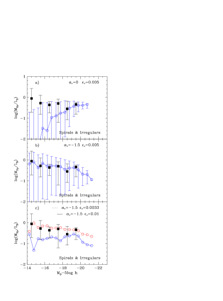
Figure 9: The cold gas content of spiral and irregular galaxies as a function of luminosity. In each panel, the filled squares and associated errorbars show observational estimates of the median, 10 and 90 percentile points respectively of the distribution of $M_{\rm Hy}/L_{\rm B}$ for Sa to Im galaxies. Here, $M_{\rm Hy}=M_{\rm HI}+M_{\rm H_{2}}$ is the mass of cold hydrogen which includes gas both in atomic and molecular forms. We have made these estimates using a combination of data from Huchtmeier & Richter ([1988]) and Sage ([1993]), as described in the text. The model results are shown by the open circles and their errorbars. For these, we select galaxies of comparable morphological type by requiring the B-band bulge-to-total luminosity ratios to be less than 0.4 . We express the model cold gas mass, $M_{\rm cold}$, in the observational units, $h^{-2}M_{\odot}$, and set $M_{\rm Hy}=0.7M_{\rm cold}$ to take account of the mass fraction of He. The upper panel shows the model with $\alpha_{\star}=0$. The middle panel shows the reference model, which has $\alpha_{\star}=-1.5$. The lower panel shows two models (the errorbars have been removed for clarity), each with $\alpha_{\star}=-1.5$, but with the parameter $\epsilon_{\star}$, which controls the star formation timescale, varied up and down from the value in the reference model.

In our model, there are two parameters, $\epsilon_{\star}$ and $\alpha_{\star}$, which determine the star formation timescale in galaxy disks (see equation 4.23). The first, $\epsilon_{\star}$, determines the star formation timescale for spiral galaxies with circular velocities comparable to those of $L_{\star}$ galaxies, while the second, $\alpha_{\star}$, determines how this timescale varies with circular velocity. The luminosity function (after rescaling by $\Upsilon$) is fairly insensitive to $\epsilon_{\star}$ and $\alpha_{\star}$, but they do strongly affect the cold gas content of galaxies.

Fig. 9 shows how the amount of cold gas present in spiral and irregular galaxies depends on galaxy luminosity. The observational data are taken from Sage ([1993]) and Huchtmeier & Richter ([1988]). The Sage ([1993]) data come from a complete sample of Sa-Sd galaxies with measurements of atomic HI and molecular $\rm H_{2}$, whereas the Huchtmeier & Richter ([1988]) data come from a complete sample of Sa-Im galaxies, but with only HI measurements. Brighter than $M_{\rm B}-5{\rm log}h<-16$, Sa-Sd galaxies dominate over Sdm-Im, and so we simply plot the Sage ([1993]) data. Fainter than $M_{\rm B}-5{\rm log}h>-16$, the mass fraction of molecular hydrogen appears to be small ($M_{\rm H_{2}}/M_{\rm HI}\la 0.2$), and so here we neglect the molecular $\rm H_{2}$ contribution and simply plot the data of Huchtmeier & Richter ([1988]). In each case, the luminosity is corrected to face-on.

The model plotted in Fig. 9a has $\alpha_{\star}=0$, corresponding to the standard Kennicutt law in which the star formation timescale is proportional to the disk dynamical time. In this case, the faint galaxies in the model typically contain less cold gas than is observed. In fact, the trend of $M_{\rm gas}/L_{\rm B}$ with $L_{\rm B}$ is in the opposite sense to that observed. The reference model plotted in Fig. 9b, has $\alpha_{\star}=-1.5$, implying longer star formation timescales for low circular velocity galaxies compared to $\alpha_{\star}=0$. This has a beneficial effect, and produces a correlation in $M_{\rm gas}/L_{\rm B}$ vs. $L_{\rm B}$ which is much closer to the data. Fig. 9c shows the effect of varying $\epsilon_{\star}$, and demonstrates how the observed gas fraction in bright spirals constrains this model parameter.

7.6 Galaxy Metallicities

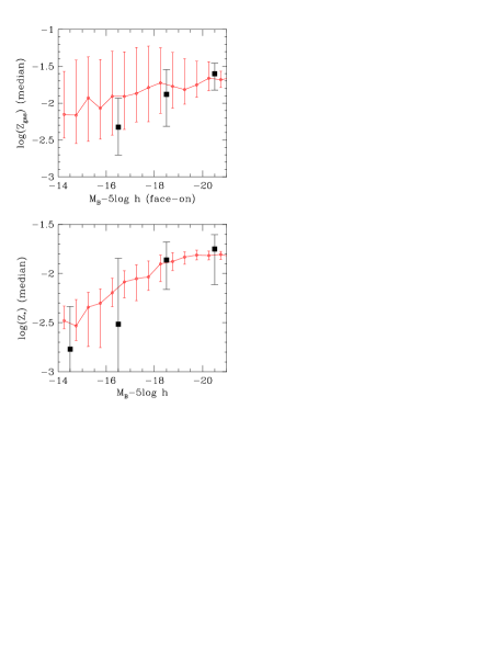
Figure 10: The dependence of metallicity on luminosity in our reference model, compared with observational data. In each panel, the lines show the median metallicity in the model and the error bars indicate the 10 and 90 percentiles of the distribution. The observational data, taken from the compilation by Zaritsky et al. ([1994]), are indicated by filled squares, where again the error bars show the 10 and 90 percentiles. The upper panel compares the metallicity of the cold star-forming gas in disk-dominated galaxies which in our model are galaxies selected to have B-band bulge-to-total ratios of less than 0.4, with observational data for spiral and irregular galaxies. The lower panel compares the stellar metallicity for bulge-dominated galaxies (B-band bulge-to-total ratios greater than 0.6) with observations for elliptical galaxies.

Our model predictions for galaxy metallicities all scale linearly with the yield $p$, aside from the effects of metallicity on the cooling of halo gas. We fix the value of $p$ in our reference model by requiring a good match to the mean stellar metallicity in $L_{\star}$ ellipticals.

In Fig. 10, we show what the reference model predicts for the metallicity-luminosity relation for spiral and elliptical galaxies, compared to observational data. Fig. 10a shows the gas metallicity vs. luminosity for spirals. The model points are derived from the metallicity of the cold, star-forming gas. The observational data in this case, from Zaritsky et al. ([1994]), are based on HII region gas metallicities measured at $r=0.4R_{25}$ in each galaxy (where $R_{25}$ is the isophotal radius at a B-band surface brightness of 25 ${\rm mag}/{\rm arcsec}^{2}$), rather than being averages over the whole galaxy. Fig. 10b shows the stellar metallicity vs. luminosity for ellipticals. The model points are obtained from mass-weighted mean stellar metallicities, but using V-band luminosity-weighted stellar metallicities would give nearly identical results. The observational data for the ellipticals are based on a compilation of estimates from line-strengths, which Zaritsky et al. have tried to put on a common metallicity scale. For both the spirals and ellipticals, we have converted the Zaritsky et al. observational data from relative to absolute metallicities assuming a solar metallicity $Z_{\odot}=0.02$.

For both the spirals and ellipticals, our models predict a metallicity-luminosity relation which is in the same sense as the observed one, but is not as steep. The origin of this correlation lies in our model of stellar feedback. Our treatment of chemical evolution differs from the traditional “closed-box” model because gas reheated by SNe is allowed to escape from the galaxy while cooling gas can flow into it. Consequently, the appropriate expression for the effective yield becomes $p_{\rm eff}=(1-e)p/(1-R+\beta)$ (equation 2.50), which depends on the strength of feedback via the quantity $\beta$ given in equation (4.24). Since $\beta$ is smaller for larger, more massive galaxies with deeper potential wells, their effective yield is large and this naturally results in more metal rich stellar populations in more luminous galaxies. We could obtain a steeper metallicity-luminosity relation, in better agreement with the observed one, by assuming stronger feedback, but this would have deleterious effects on our fits to other properties. This issue is discussed further in Section 8.3 in connection with the colour-magnitude relation.

7.7 Mass-to-Light Ratios

While the luminosities of galaxies are easily measured, the masses of the stellar populations they contain are less accurately determined, mainly because of the difficulties in separating the contributions to the mass from stars and dark matter in dynamical measurements. The mass-to-light ratios, $M/L$, for stellar populations in galaxies are correspondingly somewhat uncertain. For this reason, we do not use them as primary constraints in determining the model parameters. Nonetheless, they provide useful a consistency check, and can be used to exclude, for example, models which have very large brown dwarf fractions (i.e. large $\Upsilon$), which might otherwise be viable.

Table 2 lists the mass-to-light ratios of the stellar populations of both spiral and elliptical galaxies for each of our models. These mass-to-light ratios, which include the contribution of brown dwarfs, depend on the age and metallicity of the stellar populations, and also on the value of the parameter $\Upsilon$ which has been fixed by reference to the ${\rm b_{\rm J}}$-band luminosity function, as described in Section 7.1. Mass-to-light ratios are observed to depend on galaxy luminosity, so to make a fair comparison, we compare $M/L$ values for observed and model galaxies at the same luminosity. The model $M/L$ values given in the table are median values for $-20<M_{\rm B}-5\log h<19$. For each of the observational estimates described below, we have estimated the trend of $M/L$ with luminosity from the values given for the individual galaxies in the paper concerned, and used this to estimate the average $M/L$ for the galaxies at $M_{\rm B}-5\log h\approx-19.5$. For spiral galaxies, the observed values are dust-corrected to face-on values, and so the model $M/L$ values are also calculated from face-on luminosities including the effects of dust.

For spiral galaxies, most estimates of $M/L$ are based on fitting models to measured rotation curves. Buchhorn ([1992]) finds $M/L=3.4hM_{\odot}/L_{\odot}$ in the I-band, and Broeils ([1992]) $4.9hM_{\odot}/L_{\odot}$ in the B-band. These values are consistent with the mean colour, $B$–$I\approx 1.8$, found for spirals by de Jong ([1996]). Note, however, that these numbers are based on maximum disk fits to the observed rotation curves, and since a fraction of the rotation velocity may be produced by dark matter, they should be viewed as upper limits to the stellar mass-to-light ratios. (For $L_{\star}$ spiral galaxies in our reference model the mean contribution to the mass within the disk half-mass radius by non-baryonic dark matter is 62%.) Comparing with the model values, we see that only the model with the high value of the baryon density ($\Omega_{\rm b}=0.04$) comes close to violating these constraints. An alternative method for measuring the $M/L$ of disks, which avoids contamination by dark matter, is to combine measurements of the vertical scaleheights and velocity dispersions of galaxy disks. Using this method, Bottema ([1997]) finds an average $M/L=2.4hM_{\odot}/L_{\odot}$ in the B-band, which is about a factor of two lower than the maximum disk value. The median $M/L$ of our reference model and most of the variants are only slightly below this estimate, and so are quite compatible with observations.

The comparison for elliptical galaxies is similar. In the B-band, Mobasher et al. ([1999]) and van der Marel ([1991]) find $M/L=9.6hM_{\odot}/L_{\odot}$ and $8hM_{\odot}/L_{\odot}$ respectively, using stellar velocity dispersion measurements. Again, these values should be viewed as upper limits on the stellar mass-to-light ratios, as they include the effect of any dark matter within the effective radii of the galaxies. With the exception of the high baryon density model, all the models listed in Table 2 are consistent with these data.

7.8 Average Colours

Table 2 also lists the median $B$–$K$ colours of galaxies with $-24.5<M_{\rm K}-5\log h<-23.5$ for various parameter values. The observed median colour for this luminosity range, calculated from the data of Gardner et al. ([1996],[1997]) that are presented in Section 8.1, is $B$–$K=3.8$. The largest effects on the model colours result from varying the yield $p$, $\Omega_{\rm b}$, $\epsilon_{\star}$ and $V_{\rm hot}$. A higher yield leads both to intrinsically redder stellar populations and to greater amounts of dust, which redden the observed galaxy colours still further. Increasing $\Omega_{\rm b}$ increases the gas density in halos, and thus shortens the cooling time. This then results in a greater fraction of the gas cooling and forming stars at high redshift, producing an older, redder stellar population. Decreasing $V_{\rm hot}$ reduces the strength of feedback, allowing more stars to form in low-mass halos at high redshift, leading, again, to older, redder stellar populations by the present. Somewhat surprisingly, increasing the star formation efficiency, $\epsilon_{\star}$, (cf. equation 4.23) has little effect on the present star formation rate and galaxy colours. This happens because the shorter star formation timescale allows more star formation to occur at high redshift, and this leads to a reduction in the amount of cold star-forming gas at low redshift which compensates for the shortened star formation timescale.

The colours also depend on the choice of IMF. However, changing from the Kennicutt to the Salpeter form makes very little difference to the $B$–$K$ colours, which become bluer by just $0.015$ magnitudes. This is to be expected, as Fig. 4 demonstrates that the differences in the spectral properties of the stellar populations for these two IMFs are small. The metallicities of the stellar populations and the dust content of the galaxies are very similar in the two cases, as the adopted values of the yield are identical and of the recycled fraction almost identical.

7.9 Summary of Parameter Constraints

In this section we have demonstrated how the predictions of local galaxy properties depend on each of the model parameters. We now summarise the reasons for adopting the specific parameter values that define our standard or reference $\Lambda$CDM model.

The cosmological parameters, $\Omega_{0}=0.3$ and $\Lambda_{0}=0.7$, were chosen without reference to galaxy properties, and simply define the background cosmology in which we sought a viable model of galaxy formation. The Hubble parameter, $h=0.7$, was chosen to be in reasonable accord with recent estimates. The baryon density, $\Omega_{\rm b}$, was chosen as a compromise between constraints from primordial nucleosynthesis and the need to prevent the disks of bright galaxies becoming strongly self-gravitating and so distorting the bright end of the Tully-Fisher relation. This choice also prevents galaxies becoming too luminous, or equivalently, their $M/L$ ratios becoming too large once $\Upsilon$ has been adjusted. The shape, $\Gamma$, of the mass fluctuation power spectrum was chosen to be consistent with the above choices of $\Omega_{0}$, $\Omega_{\rm b}$ and $h$ (cf. eqn 7.36). The resulting value, $\Gamma=0.19$, is in accord with the shape of the power spectrum inferred from studies of large-scale galaxy clustering. The amplitude, $\sigma_{8}$, was chosen for consistency with the observed abundance of galaxy clusters ([1996]). For our chosen cosmology, this is consistent with the value of $\sigma_{8}$ preferred by the COBE measurements of microwave background anisotropies.

The stellar population parameters, we have essentially chosen to be consistent with models constructed to account for solar neighbourhood data. In particular, we have adopted the Kennicutt IMF. The fraction of gas recycled via stellar winds and SNe, we have taken to be $R=0.42/\Upsilon=0.31$, consistent with what is expected for this IMF. (Recall that $\Upsilon$ is defined as the total mass in stars, including brown dwarfs, divided by the mass in luminous stars. The value $\Upsilon=1.38$ was chosen by fitting the position of the bright end of the ${\rm b_{\rm J}}$-band luminosity function.) We have adopted a yield, $p=0.02$, which results in roughly the observed metallicity for galaxies similar to the Milky Way and for $L_{\star}$ ellipticals. This may be seen in Fig. 10, where we also examine the model prediction for the dependence of metallicity on galaxy luminosity. Our adopted yield implies $p_{1}\equiv p\Upsilon=0.028$, which is also roughly consistent with theoretical estimates for our assumed IMF. The yield also determines the metallicity and dust content of the cold gas disk. Our adopted value gives rise to an amount of reddening which is approximately that required to bring the model into good agreement with the observed galaxy $B$–$K$ colour distribution. Varying the IMF between the Kennicutt, Salpeter or Miller-Scalo forms has only a small effect on the galaxy colours and mass-to-light ratios at $z=0$, and so the IMF is therefore not well constrained by the data we have examined so far. However, the small differences in these IMFs can have a significant effect on model predictions at high redshift.

The dynamical friction parameter, $f_{\rm df}$, we simply set to its natural value, $f_{\rm df}=1$.

The parameter $f_{\rm ellip}$, which sets the threshold for violent galaxy mergers which produce ellipticals and bulges (cf. Section 4.3.2), was chosen so as to reproduce an acceptable mix of morphological types.

Finally, the model requires parameters for the star formation and feedback laws (cf § 4.2). The feedback parameters, $V_{\rm hot}$ and $\alpha_{\rm hot}$, we have constrained by the shape of the ${\rm b_{\rm J}}$-band luminosity function, the slope of the Tully-Fisher relation, and the distribution of spiral disk scalelengths. A low value of $\alpha_{\rm hot}$ is required to avoid curvature in the Tully-Fisher relation, while a large value helps to reduce the faint end slope of the galaxy luminosity function. Our adopted compromise, $\alpha_{\rm hot}=2$, results in a straight Tully-Fisher relation and a luminosity function with a faint end slope in good agreement with the ESP survey. This is steeper than in several other surveys, including those by Loveday et al. ([1992]) and Ratcliffe et al. ([1998]), but we have demonstrated that the slope is sensitive to surface brightness selection limits. The value of $V_{\rm hot}$ influences both the faint end of the luminosity function and the sizes of galaxies. Our adopted value of $V_{\rm hot}=200\,{\rm km\,s^{-1}}$ appears to be a good compromise. The parameter, $e$, which allows metals produced in SNe to escape directly to the surrounding hot halo gas rather than first being mixed with the cold gas in the galaxy disk, we have simply set to zero. Regarding the star formation law (equations 4.13 and 4.23), the overall scaling of the timescale, set by the efficiency $\epsilon_{\star}$, is constrained primarily by the cold gas masses in $L_{\star}$ spirals. The dependence of this timescale on galaxy circular velocity is determined by $\alpha_{\star}$. We adopted the value $\alpha_{\star}=-1.5$ in order to improve the correspondence between model and observed cold gas masses in low-luminosity disk galaxies.

8 Further properties of the reference model

In this section we compare further properties of our reference model with observational data that have not been used to set the model parameters. We defer comparisons with observations at high and moderate redshift to future papers.

Figure 11: A comparison of galaxy colours in the reference model with observations. The upper two panels compare rest-frame $B$–$K$ colour distributions in volume-limited samples for two different ranges of absolute $K$-band magnitude. The lower two panels compare the rest-frame $B$–$V$ colour distributions for the same two ranges of absolute $K$-band magnitude. In each case, the histograms with errorbars show the observational distributions, derived from the $K$-band redshift survey of Gardner et al. ([1996],[1997]) using the $1/V_{\rm max}$ method. These data have been k-corrected by matching each galaxy’s observed colours with one of a set of template spectra. If the more uncertain correction for evolution is also applied, then the observed distributions typically shift redwards by $0.15$ magnitudes. The dotted lines show the colour distribution of the reference model without including the effects of dust and the solid lines show the distributions including the effects of dust.

8.1 Colour Distributions

We have already considered the average $B$–$K$ colours of $L\sim L_{\star}$ galaxies in Section 7.8. In our reference model, the mean galaxy $B$–$K$ colour is quite strongly constrained by virtue of the requirement that the model give a reasonable fit to the bright end of both the ${\rm b_{\rm J}}$ and K-band luminosity functions. Nevertheless, it is still interesting to look at the full distribution of predicted colours, and to compare them to other observational data. In Fig. 11, the reference model is compared to the distributions of $B$–$K$ and $B$–$V$ colours in the K-selected redshift survey of Gardner et al. ([1996],[1997]). This contains more than 500 galaxies, covers 10 square degrees and was imaged in the B, V, I and K bands. The redshift and colour information allow accurate k-corrections to be derived by matching each galaxy’s observed colours with one of a set of template spectra. Thus, the histograms in Fig. 11 show rest-frame colours. If the more uncertain correction for evolution is also applied, then the observed distributions typically shift redwards by $0.15$ magnitudes. The model with dust matches both the median colours and the widths of the colour distributions quite well. If the effects of dust are not taken into account, then the resulting model median colours are too blue by approximately 0.3 magnitudes in $B$–$K$ and approximately 0.1 magnitudes in $B$–$V$. Thus, we see again how modelling the effects of dust is an important factor in producing acceptable galaxy colours.

8.2 The Colour-Morphology Relation

Figure 12: Average galaxy $B$–$V$ colour as a function of bulge-to-disk ratio, compared to observations. The open squares and error bars show the model mean $B$–$V$ colour and rms dispersion as a function of B-band bulge-to-total ratio for galaxies brighter than $M_{\rm V}-5\log h=-20.5$. Face-on colours are plotted, including the effects of extinction. The solid square shows the mean colour of model galaxies which have experienced a merger and the associated burst of star formation in the last 1 Gyr. The solid and dotted lines show the observed mean and rms dispersion of the colour from the data of Buta et al. (1994). Hubble T-type has been converted to bulge-to-total ratio using the data of Simien & de Vaucouleurs (1986), as described in Baugh et al. (1996b).

Fig. 12 shows the predicted correlation of galaxy $B$–$V$ colour, for face-on inclination, with bulge-to-disk ratio. A strong correlation is predicted, with bulge-dominated galaxies typically being much redder than disk-dominated galaxies. However, galaxies which have experienced a major merger and the associated burst of star formation within the last 1.0 Gyr have large bulge-to-disk ratios, but are much bluer than bulge-dominated galaxies that have not had a recent major merger. Observationally, “normal” galaxies show a similar trend in colour to the model galaxies which have not had recent bursts, as is illustrated by the observational data of Buta et al. ([1994]) which are also plotted, with the solid line showing the mean galaxy colour and the dotted lines showing the dispersion. Note that Buta et al. have removed from their sample some galaxies viewed as outliers or having strong emission lines. To plot these data on Fig. 12, we have converted the Hubble T-type given in Table 6 of Buta et al. to bulge-to-total ratio, using the fit given in equation (5) of Simien & de Vaucouleurs ([1986]). This fit represents an extrapolation from $T=-3$ (which corresponds to $B/T\approx 0.6$) to $T=-5$ (which corresponds to $B/T\approx 1.0$). Given the considerable scatter that exists between bulge-to-total ratio and T-type (e.g. see Figure 1. of Baugh et al. [1996b]), the level of agreement between the predictions of the model and the data is encouraging. It will be interesting to perform more quantitative comparisons of this prediction with observations when a suitable data set exists in which bulge-to-disk decompositions have been done for a complete survey.

8.3 The Elliptical Colour-Magnitude Relation

Figure 13: The colour-magnitude relation for cluster elliptical galaxies in the reference model, compared to observations. The points give the predicted distribution of V-K colour versus V-band magnitude for elliptical galaxies in clusters with circular velocity greater than $1000{\rm km\,s^{-1}}$. The heavy line and error bars indicate the median and the 20 and 80 percentiles of this distribution. The observed correlation and scatter, from Bower, Lucey & Ellis ([1992]), are indicated by the dotted line and associated error bars.

A second correlation that we have examined is the colour-magnitude relation of elliptical galaxies. This is closely related to the metallicity-luminosity relation for elliptical galaxies, already discussed in Section 7.6. Fig. 13 compares the distribution that we predict for cluster ellipticals with that determined observationally for the Coma cluster (Bower, Lucey & Ellis [1992]). The model predicts quite a small spread in the colours of bright ellipticals, consistent with the observed scatter, but it does not reproduce the strength of the observed correlation of colour with luminosity. This is the same problem that we found when we made this comparison in Baugh et al. ([1996b]), even though our new model includes chemical enrichment, which the earlier model did not.

In Kauffmann et al. ([1993]), Baugh et al. ([1996b]) and Kauffmann ([1996]), it was argued that the inclusion of chemical enrichment (which was neglected in the early models) might give rise to the desired correlation. This was explicitly demonstrated for certain models by Kauffmann & Charlot ([1998a]). In our present models, chemical enrichment does appear to have the desired effect at low luminosities, where the models produce a similar gradient in the colour-magnitude relation to the one observed. However, the correlation between metallicity and luminosity flattens at the brightest magnitudes (see Figure 10b), and this gives rise to a flattening in the predicted colour-magnitude relation for bright ellipticals. Our models are capable of producing a significant gradient in this diagram if we assume very strong feedback and a large yield $p$, just as Kauffmann & Charlot ([1998a]) did, but this is then at the expense of other successes of the model. In particular, strong feedback gives rise to excessively large disk scalelengths. This is clearly an issue that deserves further investigation.

8.4 The cosmic star formation history

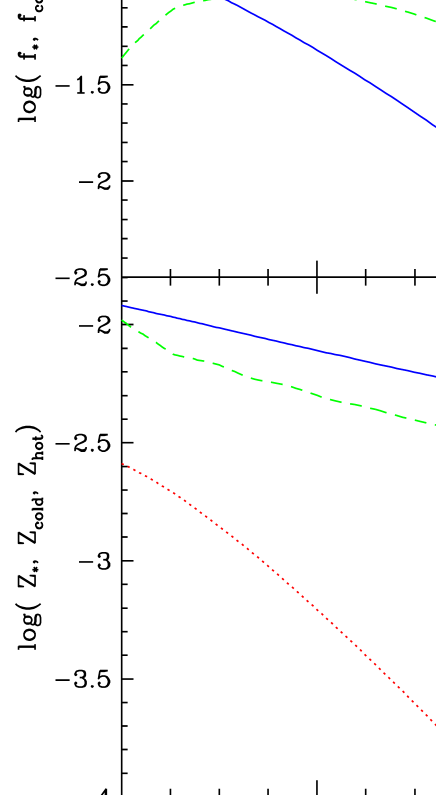
Figure 14: Evolution of baryonic mass fractions and average metallicities. The upper panel shows the fraction of baryons in stars, cold gas and hot gas as a function of redshift, and the lower panel shows their corresponding mean metallicities. The solid lines are for stars, the dashed lines for cold gas and the dotted lines for hot gas.

Figure 15: The luminous star formation rate (i.e. excluding brown dwarfs) per unit comoving volume as a function of redshift. The solid line shows the total star formation rate per unit volume in the reference model. The dashed line shows the contribution from quiescent star formation in galactic disks. The dotted line shows the contribution from bursts of star formation that occur during major mergers. The dot-dashed line is the star formation history in model G of Baugh et al. (1998) (for the same cosmological parameters as in our reference model). In the current reference model, the star formation rate per unit volume is higher at high redshift than in the old model, because of the weaker feedback in low mass halos and the shorter star formation timescale at high redshift that are assumed in the new model.

It is interesting to examine how the improvements in our modelling techniques affect our predictions for the global history of star formation, first presented in Cole et al. ([1994]). Fig. 14 shows the redshift evolution of the mass fractions of baryons in the forms of hot gas, cold gas and stars, and the mean metallicities of each of these components. Consistent with our feedback model, we have assumed that baryons contained in halos with mass below our resolution limit are in the hot, diffuse phase. We remind the reader that by “hot” gas we simply mean diffuse gas in halos, whatever its physical temperature, and by “cold” gas we mean all the gas that has cooled and collapsed into galaxies. The mass of stars increases steadily towards the present, with just over half of the present stellar mass having been formed since redshift $z<1.5$. This is similar to our earlier results in Cole et al. ([1994]) and Baugh et al. ([1998]), despite the various changes in model parameters that we discuss below. The evolution of the cold gas mass shows a broad peak between redshifts $1<z<2$. The fall-off at high redshift reflects the efficiency of stellar feedback, which keeps gas in low mass halos in the hot phase. At low redshift, the cold gas fraction begins to decline as cooling becomes increasingly less efficient in the large mass, high virial temperature groups and clusters that form at late times, while, at the same time, the reservoirs of cold gas are depleted by ongoing star formation. The mean metallicity of the hot gas grows at a rate which mirrors the growth in total stellar mass. In contrast, the mean metallicity of the stars and cold gas reaches $1/3$ of its present value even at very high redshift, and then increases only gradually between redshift $z=6$ and $z=0$.

Fig. 15 shows the star formation history in differential form. The solid line is the average formation rate of luminous stars per unit comoving volume (i.e. the total star formation rate divided by $\Upsilon$). The dashed and dotted lines show separately the contributions to the total rate from quiescent star formation in disks and from bursts of star formation induced by galaxy mergers. Approximately 10% of the stars formed at any redshift are formed in bursts.

The dot-dashed line in Fig. 15 shows our earlier result, presented as model G of Baugh et al. ([1998]). Model G had very similar cosmological parameters to the present reference model, but was calculated with a slightly earlier version of our code. The differences between the two results are easy to understand and provide a nice illustration of how various aspects of our galaxy formation modelling are closely interconnected. The main difference between the two model predictions is the lower star formation rate at high redshift obtained in model G compared to the present model. This difference mainly reflects the different values of the feedback parameters that we adopted in the two models. In our older model we set these parameters by the requirement that the faint-end of the present-day galaxy luminosity function reproduce as closely as possible that measured by Loveday et al. ([1992]). This led us in Baugh et al. (and in Cole et al. [1994]) to assume very strong feedback. Here, we have argued that the uncertainty in the faint end of the luminosity function as indicated by the wide range of observational esimates, including the very steep slope found by Zucca et al. ([1997]), suggests that this is not a robust constraint. We have instead adopted a weaker feedback that avoids introducing curvature in the faint end of the Tully-Fisher relation. Thus, in our models, the behaviour of the star formation rate at high redshift is intimately tied in with our assumptions about the strength of stellar feedback and the faint-end of the present-day galaxy luminosity function. A second difference between the present model and that of Baugh et al. ([1998]) is the assumed dependence of the star formation timescale on galaxy properties. We now incorporate a scaling with the galaxy dynamical time, which results in all star formation timescales at high redshift being smaller than in the older model. We must emphasize, however, that in spite of the uncertainties in the predicted star formation rate at high redshift, our prediction of a late epoch for the majority of star formation is robust (cf. Figure 21 of Cole et al. [1994] and Figure 14 of Baugh et al. [1998]). This is because in all the versions of our model, only a small fraction of stars form at $z>3$, and it remains the case that we expect half the stars in the universe to have formed at redshift $z\la 1.5$.

9 Discussion

In this paper, we have presented a new semi-analytic model of galaxy formation, based upon the one developed by Cole et al. ([1994]). Our new model contains a number of additions and improvements. For example, we have designed and implemented a new algorithm to generate halo merger trees with arbitrary mass resolution, and we have extended our modelling to include realistic descriptions of the density profiles of dark matter halos and their gas content, as well as calculations of chemical evolution, dust extinction, and galaxy sizes. We applied this model to a specific cosmology, the $\Lambda$CDM model, which has $\Omega_{0}=0.3$, $\Lambda_{0}=0.7$ and a primordial power spectrum whose amplitude is consistent with both the local abundance of galaxy clusters and with the COBE anisotropies in the microwave background radiation. We then compared the results with a range of observational data for the local galaxy population.

In principle, a model like ours can predict virtually any simple property of the galaxy population over a large range of redshift. However, not all predictions are equally reliable. For a given cosmological model (e.g. $\Lambda$CDM), the evolution of the population of dark matter halos is known with high accuracy and can be calculated without any free parameters. The initial internal structure of these halos is also completely specified if one adopts the results of recent high-resolution N-body simulations ([1997]). The process of gas cooling is more uncertain but can be calculated also without free parameters (other than the value of the gas metallicity), using a model based on simple assumptions about the geometry and initial configuration of the gas. We assume an initial spherically symmetric distribution of gas at the virial temperature of the halo in which it is contained, and a gas density profile given by the “$\beta$-model”. In practice, the dynamics of the cooling gas are likely to be subtantially more complex than this simple model implies. Nevertheless, as Benson et al. ([2000c]) have shown, the simple model does predict global fractions of hot and cold gas, and their distribution in halos of different mass, that are broadly in agreement with the results of gasdynamics simulations.

The formation of stars from the gas that has cooled and the associated feedback processes are the most uncertain components of the model. As in Cole et al. ([1994]), we have represented them using simple scaling laws, but we have adopted a more flexible treatment than we had done previously. In addition to specifying the IMF and the associated fraction of brown dwarfs, our model of star formation and feedback requires four free parameters. Our treatment of feedback is simplified and neglects potentially important sources of energy such as active galactic nuclei and quasars. It also neglects the dynamical response of the hot halo gas to the heating generated by the injection of feedback energy. In principle, this energy can modify the structure of the gaseous halo and hence its cooling rate. Thus, the detailed treatment of feedback impacts on all aspects of the galaxy formation model. For example, as we discussed in Section 7, our model only works well if we assume a value of the mean cosmic baryon density, $\Omega_{b}$, which is lower than recent determinations based on the deuterium abundance at high redshift by Schramm & Turner ([1998]) and Burles & Tytler ([1998]), although it is consistent with older determinations by Walker et al. ([1991]) and Copi et al. ([1995]). A larger value of $\Omega_{\rm b}$ causes too much gas to cool, leading to a poor match to the Tully-Fisher relation and to unacceptably large mass-to-light ratios. A successful model with larger values of $\Omega_{\rm b}$, however, is likely to be possible if feedback raises the entropy of the hot halo gas, thereby strongly suppressing cooling, as argued recently by Bower et al. ([2000]) in the context of X-ray clusters.

Intimately linked to the processes of star formation and feedback is the chemical evolution of the gas. Although the basic principles of chemical enrichment are well-understood, important aspects, such as the mixing of metals in the interstellar medium, remain uncertain. Our model of chemical evolution requires specifying 3 parameters, two of which, however, (the yield and the fraction of stellar mass ejected by stellar winds and SNe) are determined by the choice of IMF. The remaining parameter is related to the mixing of metals. Once the metallicity of the gas is obtained, the spectrophotometric properties of the stars are calculated using a population synthesis model which has no free parameters.

These five ingredients: gravitational evolution of halos, gas cooling, star formation and feedback, chemical evolution, and stellar population synthesis make up the core of our model of galaxy formation. To predict observable quantities, however, still requires a model for dust extinction. We assume that the mass of dust that forms is proportional to the mass in metals, and derive the extinction in any passband using a simple model for the distribution of dust in the disk. Our dust model has one free parameter (the ratio of the scaleheights of dust and stars), but our results are insensitive to its value. The core galaxy formation model can now be used to predict a wide range of visible galaxy properties including basic quantities such as the luminosity function in different passbands or the distribution of colours, as well as their evolution with redshift.

To go beyond estimates of luminosity requires the addition of more physical ingredients into the model. As the model becomes increasingly complex, it encompasses a fuller range of galaxy properties and this, inevitably, requires a growing number of physical assumptions and additional parameters. For example, it is possible to distinguish between disk and spheroidal stellar configurations by introducing simple but plausible assumptions. Here we have assumed that cooling gas settles into a centrifugally supported disk, that the distribution of halo and gas angular momentum has a particular form (consistent with results of N-body simulations), and that major mergers or disk instabilities produce spheroidal stellar systems. Our model requires one further free parameter to define what a major merger is. With these assumptions, the scalelengths of disks can be computed without further free parameters, as can the sizes of spheroids, assuming that energy is conserved in mergers.

In summary, a model of galaxy formation consists of a mixture of assumptions about the physical processes at work, together with adjustable parameters that reflect our lack of knowledge about certain complex astrophysical processes such as star formation. It is important to recognize that these parameters are not statistical variables describing a particular dataset (e.g. the faint-end slope of the luminosity function), but genuine physical quantities that describe a model for a specific physical process (e.g. the conversion of cold gas into stars). In many instances, the parameters can vary only over a relatively narrow range of physically sensible values. In our model, just as in models by other groups, we strive to make the simplest possible assumptions at every stage and to introduce the minimum number of adjustable parameters, the majority of which, in fact, are required to describe the poorly understood processes of star formation, feedback and the mixing of metals. Given the current theoretical and observational understanding of these processes, it is not possible to build a realistic model of galaxy formation which has substantially fewer parameters than ours.

Although the number of parameters is small, in any case, compared to the vast array of properties that the model can predict, it is important to adopt a well-defined, a priori methodology for fixing their values and for testing the validity of physical assumptions. In our case, this strategy is straightforward: we fix the values of all the parameters by attempting to match a small subset of the local galaxy data which we regard as the most fundamental. In order of the weight we give them, these are: the luminosity functions in the B- and K-bands; the relative fractions of ellipticals, S0s, and spirals; the slope of the Tully-Fisher relation at faint magnitudes; gas fractions in disks as a function of B-band luminosity; the distribution of disk sizes; and the metallicity of $L_{\star}$ ellipticals. Once the model parameters have been set by these comparisons, we test our model predictions against a wide range of other data, without any further adjustments.

The galaxy formation model presented here differs in several significant respects from that of Cole et al. ([1994]). That model was based on a cruder method for generating halo merger trees, but that alone makes little difference to the resulting galaxy properties. Similarly, the extensions we have included which allow us to predict more galaxy properties, such as sizes and mean metallicities, make little difference to the properties that we were able previously to predict. There are three differences which do lead to significant changes in our results. Firstly, the adoption of a cosmological model with a low value of $\Omega_{0}$ reduces the number of galaxy-sized halos, and this helps to reduce the offset in the Tully-Fisher relation for models normalized to the B-band luminosity function (see [1995]). Secondly, the inclusion of dust in the calculation of luminosities and colours makes a typical galaxy colour slightly redder and this helps to match the B and K-band luminosity functions simultaneously. Furthermore, since the luminosities that enter into the I-band Tully-Fisher relation are partially corrected for the effects of extinction, the inclusion of dust also helps reduce the offset between model and data seen in Cole et al. ([1994]). Thirdly, we have adopted a weaker feedback law for low circular velocity galaxies, since some recent determinations of the galaxy luminosity function indicate that the very flat faint-end which we strived hard to match in Cole et al. ([1994]) is not a robust observational constraint and may be affected by survey selection criteria. This, in turn, implies a higher star formation rate at redshifts $z\ga 3$.

Although in this paper we have focussed on the $\Lambda$CDM model, we have also investigated models with other values of the cosmological parameters. For reasons of space, we do not present our results in any detail here, but confine ourselves instead to a few general remarks, applicable to cluster-normalized models. A standard CDM model (SCDM, $\Omega_{0}=1$) still fails to match the Tully-Fisher relation (even using halo circular velocities) and the luminosity function simultaneously. An $\Omega_{0}=1$ model with the same power spectrum shape as $\Lambda$CDM (the $\tau$CDM model of Jenkins et al. [1998]) shares this problem and, in addition, the smaller amount of small-scale power compared to SCDM results in a later epoch for the onset of galaxy formation and, thus, in both a lower star formation rate density and a lower abundance of Lyman-break galaxies at high redshift. (This problem does not afflict the $\Lambda$CDM model because the effect due to the shape of the power spectrum is compensated for by the difference in the linear growth rate and the higher initial amplitude required by the cluster normalization.)

There are now in the literature a number of semi-analytic galaxy formation models of varying sophistication, based on similar principles to ours (e.g. Avila-Rees & Firmani [1998], Guiderdoni et al. [1998], Roukema [1998], Wu et al. [1998], Kauffmann et al. [1999a], Somerville & Primack [1999]). It is beyond the scope of this paper to carry out a detailed comparison of all these models, but we refer the reader to the recent paper by Somerville & Primack ([1999]) which has compared some of the different approaches, including those of the Durham, Munich, and Santa-Cruz groups. For the most part, results from different models tend to agree well when similar assumptions are made. In practice, however, it is not uncommon for different groups to make somewhat different assumptions and, most importantly, to include different physical effects in their models. This naturally leads to different results. An example of the former are the different strategies for constraining the star formation and feedback laws adopted by Kauffmann et al. ([1999a]) and ourselves. We give most weight to the local B-band luminosity function and do not make any further adjustments when calculating the zero-point of Tully-Fisher relation. By contrast, Kauffmann et al. ([1999a]) give most weight to the zero-point of the Tully-Fisher relation. Since the models do not match both these observables perfectly, there is a difference in the luminosity normalization of the two models that propagates to other observables. An example of different physical processes is the treatment of the structure and angular momentum transport of gas cooling onto galaxies adopted by Wu et al. ([1998]). Their model leads to a completely different mechanism for making ellipticals and spirals to the one operating in our own model or in that of Kauffmann et al. ([1999a]).

10 Conclusions

We have presented a new semi-analytic model of galaxy formation which contains several novel features. It employs a state-of-the art Monte-Carlo algorithm for calculating the merging evolution of dark matter halos and it incorporates, for the first time, detailed prescriptions for calculating the sizes of disks and spheroids. We used this model to calculate observable properties of galaxies in the $\Lambda$CDM cosmology ($\Omega_{0}=0.3$, $\Lambda_{0}=0.7$, $h=0.7$, and $\sigma_{8}=0.93$) and focussed primarily on galaxy properties at the current epoch, with the following main conclusions:

• A pleasing agreement can now be obtained between the model and observed galaxy luminosity functions in the B-band and the K-band, over at least 8 magnitudes. This is a non-trivial success. In the B-band, the model was tuned to fit the ESP luminosity function of Zucca et al. ([1997]), which has a steep faint-end. Unfortunately, there is still a large uncertainty in the observational estimate of the number of galaxies fainter than $L_{\star}$. This is disappointing because the faint-end slope of the luminosity function is extremely sensitive to feedback processes which are therefore only crudely constrained. A flatter faint-end, like that measured, for example, by Loveday et al. ([1992]) in the Stromlo-APM survey, could be obtained by increasing the strength of feedback. Our inability to constrain the feedback model better has a knock-on effect on our ability to predict the cosmic star formation rate at high redshift since this too is strongly influenced by feedback. Dust extinction has a relatively modest effect, dimming the bright end of the B-band luminosity function by about 0.5 mag. We showed that surface brightness effects can be important for faint galaxies, and this could help explain some of the discordant estimates of the faint end of the luminosity function.

• Our model reproduces both the observed mean galaxy colours and the spread in colour over a large range of galaxy luminosity. The stellar mass-to-light ratios of both stellar disks and ellipticals match the observational values well. Inclusion of reddening is important for this comparison, which does not involve adjusting any model parameters. The mean and scatter in the colours of galaxies of different morphological types, as measured by blue bulge-to-total light ratio, are also reproduced well.

• The current cold gas content of galaxies of different luminosity is related to the efficiency of past and current star formation. Our adopted star formation model (which is consistent with the observations analysed by Kennicutt [1998]) leads to excellent agreement with the observed ratio of cold gas mass to blue luminosity over 7 magnitudes.

• The predicted distribution of disk sizes is sensitive to the strength of feedback. Our model agrees well with the data, particularly for bright galaxies.

• The more realistic treatment of various properties and processes (e.g. dark halo and gas density profiles, dust, etc) leads to a better match to the I-band Tully-Fisher relation than was possible with our earlier, simpler model. If, as in most previous work of this kind, the circular velocity of a galaxy is identified with the circular velocity at the virial radius of the halo in which it formed, then our model gives an excellent fit to the zero-point, slope and scatter of the Tully-Fisher relation. However, in the model, the rotation velocities of galaxy disks at their half-mass radii are typically 30% higher than the circular velocities of the halos at the virial radius. This results in an offset of $+30$% in the velocity zero-point of the Tully-Fisher relation when the calculated disk velocities are used. It remains unclear whether this disagreement reflects a fundamental shortcoming of the cold dark matter theory or whether it is simply a reflection of various physical uncertainties in the calculation. For example, the derived disk rotation velocity depends on the assumptions of angular momentum conservation and adiabatic invariance during the collapse and formation of a galactic disk. If the collapse were, in fact, clumpy, then angular momentum would be transferred from the disk to the halo (Frenk et al. [1985], Navarro & White [1994], Navarro & Steinmetz [1997]). In this case our calculation may have overestimated the amount by which the inner part of the halo contracts. This would help reduce the Tully-Fisher offset, but at the same time the loss of angular momentum from the disk would make the disks physically smaller and could act in the opposite direction, compressing the halo more strongly. These issues are worthy of further investigation, but they are best addressed using numerical simulations (see e.g. [1999]).

• Our model calculates chemical evolution, taking into account the effects of gas loss due to winds and gas accretion due to cooling in a self-consistent way. The model predicts a trend of increasing metallicity with luminosity, similar to that observed, for star-forming gas in disk-dominated galaxies and for stars in bulge-dominated galaxies. However, the colour-magnitude relation for ellipticals in clusters is significantly flatter than observed at bright magnitudes, although the scatter is about right. Kauffmann & Charlot ([1998a]) have shown that a steeper slope for the colour-magnitude relation can be obtained by simultaneously increasing the strength of the feedback and the value of the yield. However, in our $\Lambda$CDM model, a much stronger feedback than we have assumed would result in disk sizes that are much too large (because the accretion of gas onto galaxies is delayed), and would degrade the fit to the Tully-Fisher relation. We intend to carry out a more thorough investigation of this conflict in a later paper.

• Our more sophisticated modelling techniques do not change our earlier conclusion (Cole et al. [1994], Baugh et al. [1998]) that half of the stars in the universe formed since $z\la 1.5$. However, the relaxation of the requirement for strong feedback (arising from the fact that we now fit the steep faint-end slope of the ESP luminosity function rather than the flat slope of the Stromlo-APM survey) allows a somewhat higher star formation rate at $z\ga 3$ than we had predicted previously. The fraction of baryons in cold gas has a broad peak at $1<z<2$. The evolution of the mean metallicity of the hot gas mirrors the growth of stellar mass but, as noted also by Kauffmann ([1996]), the mean metallicity of the stars and cold gas builds up very rapidly: it is already about one third of the present value at $z=5$.

In summary, the model we have presented is broadly successful in matching a large range of galaxy properties. There remain, however, some interesting discrepancies, for example, the Tully-Fisher relation and the colour-magnitude relation for cluster ellipticals. Although the discrepancies are relatively small, further work is required to assess whether they point to incorrect assumptions or to the neglect of important physical processes in our modelling procedure.

Appendix A Halo Rotation Velocity

In this appendix we relate the halo rotation velocity, $V_{\rm rot}$, (assumed constant) to its spin parameter $\lambda_{\rm H}$.

The total angular momentum of the halo is given by

$$J_{\rm H}({r_{\rm vir}})=\int_{0}^{r_{\rm vir}}\frac{\pi}{4}V_{\rm rot}\,r^{\prime}\,\rho(r^{\prime})\,4\pi r^{\prime 2}dr^{\prime}.$$ (1.37)

The total energy of the halo within the virial radius is the sum, $E_{\rm H}=W_{\rm H}+T_{\rm H}$, of the potential and kinetic energies. The self-binding energy of the material within the virial radius, ${r_{\rm vir}}$, is

$$W_{\rm H}({r_{\rm vir}}) = \frac{1}{2}\int_{0}^{r_{\rm vir}}\phi(r^{\prime})\,\rho(r^{\prime})\,4\pi r^{\prime 2}\,dr^{\prime}$$ (1.38)

$$= -\frac{1}{2{\rm G}}\int_{0}^{\infty}|\nabla\phi(r^{\prime})|^{2}r^{\prime 2}\,dr^{\prime}$$

$$= -\frac{{\rm G}}{2}\left[\int_{0}^{r_{\rm vir}}\frac{M(r^{\prime})^{2}}{r^{\prime 2}}\,dr^{\prime}+\frac{M^{2}({r_{\rm vir}})}{{r_{\rm vir}}}\right],$$

where $\phi(r)$ is the gravitational potential. Assuming hydrostatic equilibrium with an isotropic velocity dispersion $\sigma(r)$, the corresponding kinetic energy of material inside the virial radius can be expressed as

$$T_{\rm H}({r_{\rm vir}})=\int_{0}^{r_{\rm vir}}\frac{3}{2}\sigma^{2}(r^{\prime})\,\rho(r^{\prime})\,4\pi r^{\prime 2}\,dr^{\prime}.$$ (1.39)

With the same assumptions, the velocity dispersion obeys the Jeans equation $d(\rho\sigma^{2})/dr=-\rho\,GM(r)/r^{2}$. Provided that $r^{3}\rho(r)\sigma^{2}(r)$ vanishes as $r\to 0$ we obtain,

$$T_{\rm H}({r_{\rm vir}}) = 2\pi\Big{[}r_{\rm vir}^{3}\,\rho({r_{\rm vir}})\,\sigma^{2}({{r_{\rm vir}}})$$ (1.40)

$$+ \int_{0}^{r_{\rm vir}}{\rm G}M(r^{\prime})\,\rho(r^{\prime})\,r^{\prime}\,dr^{\prime}\Big{]}.$$

For our standard case of halos with the NFW density profile, equation (3.8), we simply integrate the Jeans equation out to $r=\infty$ to derive $\sigma(r)$, assuming that the NFW profile and hydrostatic equilibrium apply at all radii (Cole & Lacey ([1996]), equation (2.14)). This is an approximation, since in principle we should not expect the NFW halo model to be valid beyond the virial radius, where material is still infalling. However, the velocity dispersion within the halo derived in this way using the NFW model has been found to be in good agreement with numerical simulations (e.g. figures 4, 5 and 6 of Cole & Lacey [1996]). Note also that truncating the NFW profile at the virial radius implies that $2T_{\rm H}({r_{\rm vir}})+W_{\rm H}({r_{\rm vir}})\neq 0$. If the integrals in equations (1.38) and (1.40) were extended to $r=\infty$ then the NFW halo model would exactly satisfy the virial theorem, but for the truncated model $2T({r_{\rm vir}})/|W({r_{\rm vir}})|$ is slightly greater than unity and varies slowly with the NFW scalelength, $a_{\rm NFW}$. This behaviour was also found for the N-body halos in Cole & Lacey ([1996]) and our definitions are fully consistent with the way in which they defined the spin parameter $\lambda_{\rm H}$.

Inserting the above definitions of $J_{\rm H}({r_{\rm vir}})$ and $E_{\rm H}({r_{\rm vir}})$ into equation (3.6) for $\lambda_{\rm H}$ defines the coefficient $A(a_{\rm NFW})$ in the relation

$$V_{\rm rot}=A(a_{\rm NFW})\lambda_{\rm H}V_{\rm H},$$ (1.41)

where $V_{\rm H}\equiv(GM/{r_{\rm vir}})^{1/2}$ is the circular velocity of the halo at the virial radius. For the limited range $0.03<a_{\rm NFW}<0.4$ the result is well fit by $A(a_{\rm NFW})\approx 4.1+1.8\,a_{\rm NFW}^{5/4}$.

For the non-standard case of an isothermal density profile for the halo (with or without a core radius), we follow a slightly different approach. If, as above, the kinetic energy, $T_{\rm H}({r_{\rm vir}})$, is calculated by integrating the Jeans equation to derive $\sigma(r)$, then $2T_{\rm H}({r_{\rm vir}})/|W_{\rm H}({r_{\rm vir}})|$ is found to be considerably greater than unity. The discrepancy is large because we have extrapolated the halo density profile beyond the virial radius with a model whose mass does not rapidly converge. Thus, for these profiles, we prefer to define the coefficient, $A$, in equation (1.41) by evaluating the binding energy, expression (1.38), with the appropriate density profile but then assuming the virial theorem, $2T_{\rm H}({r_{\rm vir}})/|W_{\rm H}({r_{\rm vir}})|=1$, to estimate the kinetic energy and hence the total energy $E_{\rm H}({r_{\rm vir}})$. This is then identical to the assumption made in Mo et al. ([1998a]) to define the energy and spin parameter. In the range $0.01<a<0.4$ the resulting dependence is well fit by $A\approx 3.66-0.83\,a$.

Appendix B Star Formation

The set of coupled differential equations,(4.15-4.20), describing an episode of star formation has the following analytic solutions. The mass of gas that has cooled and been accreted in a time $t$ since the start of the timestep is

$$\Delta M_{\rm acc}=\dot{M}_{\rm cool}\ t.$$ (2.42)

The increase in the mass of long lived stars

$$\Delta M_{\star}=M^{0}_{\rm cold}\frac{1-R}{1-R+\beta}\ \left[1-\exp(-t/\tau_{\rm eff})\right]$$

$$-\dot{M}_{\rm cool}\tau_{\rm eff}\frac{1-R}{1-R+\beta}\ \left[1-t/\tau_{\rm eff}-\exp(-t/\tau_{\rm eff})\right]$$ (2.43)

where $\tau_{\rm eff}=\tau_{\star}/(1-R+\beta)$ . In terms of these quantities the changes in the masses of cold and hot gas are

$$\Delta M_{\rm cold}=\Delta M_{\rm acc}-\frac{1-R+\beta}{1-R}\Delta M_{\star}$$ (2.44)

and

$$\Delta M_{\rm hot}=-\Delta M_{\rm acc}+\frac{\beta}{1-R}\Delta M_{\star}.$$ (2.45)

The corresponding changes in the masses of metals are

$$\Delta M^{Z}_{\rm cold}=\Delta M^{Z}_{\rm acc}+\frac{(1-e)p}{1-R}\Delta M_{\star}-\frac{1-R+\beta}{1-R}\Delta M^{Z}_{\star}$$ (2.46)

$$\Delta M^{Z}_{\rm hot}=-\Delta M^{Z}_{\rm acc}+\frac{ep}{1-R}\Delta M_{\star}+\frac{\beta}{1-R}\Delta M^{Z}_{\star},$$ (2.47)

where

$$\Delta M^{Z}_{\rm acc}=\dot{M}_{\rm cool}Z_{\rm hot}\ t$$ (2.48)

and

$$\Delta M^{Z}_{\star}=\frac{1-R}{1-R+\beta}\Big{(}M^{Z0}_{\rm cold}\left[1-\exp(-t/\tau_{\rm eff})\right]$$

$$-\dot{M}_{\rm cool}\tau_{\rm eff}Z_{\rm hot}\left[1-t/\tau_{\rm eff}-\exp(-t/\tau_{\rm eff})\right]$$

$$+\frac{(1-e)p}{1-R+\beta}\Big{[}M^{0}_{\rm cold}\left[1-(1+t/\tau_{\rm eff})\exp(-t/\tau_{\rm eff})\right]$$

$$-\dot{M}_{\rm cool}\tau_{\rm eff}\left[2\negthinspace-\negthinspace t/\tau_{\rm eff}\negthinspace-\negthinspace(2\negthinspace+\negthinspace t/\tau_{\rm eff})\exp(-t/\tau_{\rm eff})\right]\Big{]}\Big{)}$$ (2.49)

For the case where there is no supply of cooling gas, $\dot{M}_{\rm cool}=0$, the above equations show that when $t\gg\tau_{\rm eff}$, the mean metallicity of the stars that have formed is

$$Z_{\star}=Z_{\rm cold}^{0}+\frac{(1-e)p}{1-R+\beta}.$$ (2.50)

Thus our model of star formation and feedback produces an effective yield $p_{\rm eff}=(1-e)p/(1-R+\beta)$ which, through $\beta$, and possibly also $e$, is a function of the potential well depth of the galaxy disk or bulge in which the star formation is occuring.

Appendix C Adiabatic Contraction of Halo, Disk and Spheroid

This appendix describes how we use the adiabatic contraction model to calculate the dynamical equilibrium of the disk, bulge and halo. The outputs from the calculation are the disk and bulge radii and the halo density profile after deformation by the gravity of the disk and spheroid.

C.1 Adiabatic Contraction of Halo

To model the effect on the halo density profile of a galaxy condensing at its centre, we start by assuming that baryons and dark matter have the same initial density distribution, with total mass profile, $M_{\rm H0}(r_{0})$ (e.g. given by the NFW profile). A fraction $1-f_{\rm H}$ of the total mass condenses to form a galaxy at the centre of the halo, leaving a fraction $f_{\rm H}$ of the mass still in the halo component. This fraction includes any baryons that have not yet cooled and also satellite galaxies. For simplicity, any baryons left in the hot component are assumed to be distributed like the dark matter. We now assume that in response to the gravity of the disk and the bulge, each shell of halo matter adjusts its radius to conserve its pseudo specific angular momentum $rV_{\rm c}(r)$, i.e. that $rV_{\rm c}(r)$ is an adiabatic invariant. Thus,

$$r_{0}V_{\rm c0}(r_{0})=rV_{\rm c}(r)$$ (3.51)

where $V_{\rm c}(r)$ is the total circular velocity at radius $r$, $r_{0}$ is the radius of a shell before condensation of the galaxy, and $r$ is the final radius of the same shell after condensation of the galaxy. The initial and final halo masses interior to the shell are related by

$$M_{\rm H}(r)=f_{H}M_{\rm H0}(r_{0}),$$ (3.52)

where $M_{\rm H}(r)$ is the final mass halo profile. For the purpose of computing the circular velocity of the halo (averaged over spherical shells), we treat the mass distribution (including the disk) as spherical. This should be a better approximation for estimating the gravitational influence of the disk on the halo, than using the circular velocity due to the disk in the disk plane, which is somewhat larger. Thus,

$$V_{\rm c}^{2}(r)=G\left[M_{\rm H}(r)+M_{\rm D}(r)+M_{\rm B}(r)\right]/r,$$ (3.53)

where $M_{\rm D}(r)$ and $M_{\rm B}(r)$ are the disk and bulge masses interior to radius $r$. For consistency, the total masses should be related by $M_{\rm H0}=f_{\rm H}M_{\rm H0}+M_{\rm D}+M_{\rm B}$, so that the outer radius of the halo is unchanged. Combining (3.51), (3.52) and (3.53) we have,

$$r_{0}M_{H0}(r_{0})=r\left[f_{H}M_{\rm H0}(r_{0})+M_{D}(r)+M_{B}(r)\right],$$ (3.54)

which relates the final radius of any halo shell to its initial radius, once the galaxy disk and bulge profiles, $M_{\rm D}(r)$ and $M_{\rm B}(r)$, are known. The accuracy of this approach has recently been tested in Navarro & Steinmetz ([2000]).

C.2 Dynamical Equilibrium of Disk and Bulge

Application of the galaxy rules described in Section 4.1 give the total mass, $M_{\rm D}$, and specific angular momentum, $j_{\rm D}$, of a galaxy disk, but, in order to use (3.54), we require the complete mass profile, $M_{\rm D}(r)$. To obtain this we make the following simplifying assumptions. First, we assume that all disks are well-described by an exponential surface density profile,

$$\Sigma_{\rm D}(r)={M_{\rm D}\over 2\pi h_{\rm D}^{2}}\,\exp(-r/h_{\rm D}),$$ (3.55)

for which

$$M_{\rm D}(r)=M_{\rm D}\left[1-(1+r/h_{\rm D})\,\exp(-r/h_{\rm D})\right].$$ (3.56)

The half-mass radius, $r_{\rm D}$, is related to the scalelength, $h_{\rm D}$, by $r_{\rm D}=1.68h_{\rm D}$. We also assume that the specific angular momentum of the disk is given by

$$j_{\rm D}=k_{\rm D}r_{\rm D}V_{\rm cD}(r_{\rm D}),$$ (3.57)

where $V_{\rm cD}(r_{\rm D})$ is the circular velocity in the disk plane at the disk half-mass radius and $k_{\rm D}$ is a constant. We adopt $k_{\rm D}=1.19$ as is appropriate for a flat rotation curve. The value of $k_{\rm D}$ is only weakly dependent on the assumed rotation curve. For example, if $V_{\rm cD}(r)$ is taken to be the circular velocity of a self-gravitating exponential disk (Binney & Tremaine [1987] eq. 2-169), then $k_{\rm D}=1.09$, while if $V_{\rm cD}(r)\propto 1/r^{1/2}$, then $k_{\rm D}=1.03$.

The radius of the disk is then related to its angular momentum by

$$j_{\rm D}^{2} = k_{\rm D}^{2}r_{\rm D}^{2}V_{\rm cD}^{2}(r_{\rm D})$$ (3.58)

$$= k_{\rm D}^{2}Gr_{D}\left[f_{\rm H}M_{\rm H0}(r_{\rm D0})+\frac{1}{2}k_{\rm h}M_{\rm D}+M_{\rm B}(r_{\rm D})\right],$$

where $r_{\rm D0}$ is the initial radius of the shell whose final radius is $r_{\rm D}$. The factor $k_{\rm h}$ arises from the disk geometry; if the disk contribution to $V_{\rm cD}(r)$ is computed in the spherical approximation, $k_{\rm h}=1$, but here instead we calculate the circular velocity in the midplane of the exponential disk, using equation (2-169) from Binney & Tremaine ([1987]), giving $k_{\rm h}=1.25$.

The disk half-mass radius, $r_{\rm D}$, must satisfy this equation and also equation (3.54) evaluated at $r_{\rm D}$, i.e.

$$r_{\rm D0}M_{\rm H0}(r_{\rm D0}) =$$ (3.59)

$$r_{\rm D} \negthinspace\negthinspace\negthinspace\negthinspace\negthinspace\negthinspace\Big{[}f_{\rm H}M_{\rm H0}(r_{\rm D0})+\frac{1}{2}M_{\rm D}+M_{\rm B}(r_{\rm D})\Big{]}.$$

Using (3.58), this can be written as

$$r_{D0}M_{H0}(r_{D0})=\frac{j_{D}^{2}}{k_{D}^{2}G}-\frac{1}{2}(k_{h}-1)r_{D}M_{D}.$$ (3.60)

To derive the size of the spheroidal component of a galaxy, we assume that the projected density profile is well described by the de Vaucouleurs $r^{1/4}$-law (e.g. Binney & Tremaine [1987], (§1-13)). The effective radius, $r_{\rm e}$, of the $r^{1/4}$-law (the radius that contains half the mass in projection) is related to the half-mass radius, $r_{\rm B}$, by $r_{\rm B}=1.35r_{\rm e}$. We define a pseudo-specific angular momentum for the spheroid:

$$j_{\rm B}=r_{\rm B}V_{\rm c}(r_{\rm B}),$$ (3.61)

where $V_{\rm c}(r)$ is the circular velocity at $r$. This pseudo-specific angular momentum, $j_{\rm B}$, is assumed to be conserved, except during galaxy mergers, when its value is determined by the properties of the merger remnant (see Section 4.4.2).

This model leads to the following two equations for the bulge radius, in analogy to equations (3.58) and (3.60) for the disk radius,

$$j_{\rm B}^{2} = r_{\rm B}^{2}V_{\rm c}^{2}(r_{\rm B})$$ (3.62)

$$= Gr_{\rm B}\left[f_{\rm H}M_{\rm H0}(r_{\rm B0})+M_{\rm D}(r_{\rm B})+\frac{1}{2}M_{\rm B}\right]$$

and

$$r_{\rm B0}M_{\rm H0}(r_{\rm B0})=\frac{j_{\rm B}^{2}}{G}.$$ (3.63)

Comparing this last equation to the analogous equation for the disk, (3.60), we see that the 2nd term on the RHS has vanished. This results from assuming that the mean effect of the disk on a spherical shell of the spheroid can be estimated by spherically averaging the disk.

To compute the disk and bulge radii we must solve equations (3.58), (3.60), (3.62) and (3.63) given the disk and bulge masses, $M_{\rm D}$ and $M_{\rm B}$, the initial halo profile, $M_{\rm H0}(r_{0})$, and specific angular momenta, $j_{\rm D}$ and $j_{\rm B}$. The two pairs of equations are coupled, but with care they can be solved with a simple iterative scheme.

C.3 Adiabatic Adjustment following Mergers or Disk Instabilities

When a spheroid is formed by a galaxy merger, we first calculate the radius of the new spheroid $r_{\rm new}$ from (4.28). We then compute $j_{\rm B}=r_{\rm B}V_{\rm c}(r_{\rm B})$, with $r_{B}=r_{\rm new}$ and $V_{\rm c}^{2}(r_{\rm B})=G(M_{1}+M_{2})/2r_{\rm new}$. Then, using this value of $j_{\rm B}$, we calculate the value of $r_{\rm B}$ given by the adiabatic contraction model for the disk-bulge-halo equilibrium, and take this be the true value of $r_{\rm B}$. If a spheroid is formed via disk instability, we follow the same procedure, starting from $r_{\rm new}$ given by equation (4.31), and assuming that the dark matter mass involved in the initial calculation of $V_{\rm c}^{2}(r_{\rm B})$ is twice that within the initial half-mass radius of the galaxy.

References

- [1998] Adelberger, K.L., Steidel, C.C., Giavalisco, M., Dickinson, M., Pettini, M., Kellogg, M., 1998, ApJ, 505, 1
- [1998] Avila-Reese, V., Firmani, C., 1998, ApJ, 505, 37
- [2000] Balbi, E., et al. , 2000, ApJL, submitted. (astro-ph/0005124)
- [1992] Barnes, J. 1992, Ap.J. 393, 484
- [1987] Barnes, J.E., Efstathiou, G., 1987, ApJ, 319, 575
- [1984] Barnes, J.E., White, S.D.M., 1984, MNRAS 211,753
- [1998] Barnes, J.E., 1998, in Galaxies: Interactions and Induced Star Formation, Saas-Fee Advanced Course 26. Lecture Notes 1996. Swiss Society for Astrophysics and Astronomy, XIV, Edited by R. C. Kennicutt, Jr. F. Schweizer, J. E. Barnes, D. Friedli, L. Martinet, and D. Pfenniger. Springer-Verlag Berlin/Heidelberg, p.275,
- [1996a] Baugh, C.M., Cole, S., Frenk, C.S., 1996a, MNRAS, 282, L27
- [1996b] Baugh, C.M., Cole, S., Frenk, C.S., 1996b, MNRAS, 283, 1361
- [1998] Baugh, C.M., Cole, S., Frenk, C.S., Lacey, C.G., 1998, ApJ, 498, 504
- [1999] Baugh, C.M., Benson, A.J., Cole, S., Frenk, C.S., Lacey, C.G., 1999, MNRAS, 305, L21
- [2000a] Benson, A.J., Cole, S., Frenk, C.S., Baugh, C.M., Lacey, C.G., 2000a, MNRAS, 311, 793
- [2000b] Benson, A.J., Baugh, C.M., Cole, S., Frenk, C.S., Lacey, C.G., 2000b, MNRAS, in press. (astro-ph/9910488)
- [2000c] Benson, A.J., Pearce, F.R., Frenk, C.S., Baugh, C.M. Jenkins, A., 2000c, MNRAS, submitted (astro-ph/9912220).
- [2000] de Bernardis,P., et al. 2000, Nature, 404, 955
- [1987] Binney, J., Tremaine, S., 1987, “Galactic Dynamics”, Princeton University Press, Princeton, New Jersey
- [2000] Blanton, M., Cen, R., Ostriker, J.P., Strauss, M.A., Tegmark M., 2000, ApJ, 531, 1
- [1984] Blumenthal, G., Faber, S., Primack, J., Rees, M., 1984, Nature, 311, 517
- [1986] Blumenthal, G., Faber, S., Flores, R., Primack, J., 1986, ApJ, 301, 27
- [1991] Bond, J.R., Cole, S., Efstathiou, G., Kaiser, N., 1991, ApJ, 379, 440
- [1997] Bond, J.R., Efstathiou, G., Tegmark, M., 1997, MNRAS 291, 33
- [1999] van den Bosch, F., Lewis, G.F., Lake, G., Stadel, J., 1999, ApJ 515, 50
- [1997] Bottema, R., 1997, A&A, 328, 517
- [1991] Bower, R.J., 1991, MNRAS, 248, 332
- [1992] Bower, R.G., Lucey, J.R., Ellis, R.S., 1992, MNRAS, 254, 601
- [2000] Bower, R.G., Benson, A.J., Baugh, C.M., Cole, S., Frenk, C.S., Lacey, C.G., 2000, MNRAS, submitted. (astro-ph/0006109)
- [1994] Bressan, A., Chiosi, C., Fagotto, F., 1994, ApJS, 94, 63
- [1992] Broeils, A.H., 1992, PhD thesis, Groningen
- [2000, in preparation] Bruzual, A.G., Charlot, S., 2000, in preparation.
- [1993] Bruzual, A.G., Charlot, S., 1993, ApJ, 405, 538
- [1992] Buchhorn, M., 1992, PhD thesis, ANU
- [1999] Bullock, J.S., Kolatt T.S., Sigad Y., Somerville, R.S., Kravtsov A.V., Klypin A.A., Primack, J.R., Dekel, A., 1999, MNRAS, submitted (astro-ph/9908159)
- [1998] Burles S., Tytler, D., 1998, Sp. Sc. Rev., 84, 65
- [1994] Buta, R., Mitra S., de Vaucouleurs G., Corwin H.G., 1994, AJ, 107, 118
- [1976] Cavaliere, A., Fusco-Femiano R., 1976, A&A, 94, 137
- [1996] Charlot, S., Worthey, G., Bressan, A., 1996, ApJ, 57, 625
- [1995] Christodoulou, D.M., Shlosman, I., Tohline, J.E., 1995, ApJ, 443, 563
- [1991] Cole, S., 1991, ApJ, 367, 45
- [1994] Cole, S., Aragón-Salamanca, A., Frenk, C.S., Navarro, J.F., Zepf, S.E., 1994, MNRAS, 271, 781
- [1996] Cole, S., Lacey, C.G., 1996, MNRAS, 281, 716
- [1997] Cole, S., Weinberg D.H., Frenk C.S., Ratra B., 1997, MNRAS, 289, 37
- [1999] Colpi, M., Mayer, L., Governato, F., 1999, ApJ, 525, 720
- [1990] Combes, F., Debbusch, F., Friedli, D., Pfenniger, 1990, A&A, 233, 82
- [1999] Combes, F., 1999, in proceedings of Rencontres de Moriond, “Building Galaxies: from the Primordial Universe to the Present”, ed F. Hammer, T. X. Thuan, V. Cayatte, B. Guiderdoni and J. Tran Thanh Van (astro-ph/9904031)
- [1995] Copi, C. J., Schramm, D. N. & Turner, M. S., 1995, ApJL, 455, L95
- [1999] Croft, R.A.C, Weinberg, D.H., Pettini, M., Hernquist, L., Katz, N., 1999, ApJ, 520, 1
- [1985] Davis, M., Efstathiou, G., Frenk, C.S., White, S.D.M., 1985, ApJ., 292, 371
- [1982] Efstathiou, G., Lake, G., Negroponte, J., 1982, MNRAS, 199, 1069
- [1988] Efstathiou, G., Frenk C.S., White S.D.M., Davis M., 1988, MNRAS, 235, 715
- [1996] Eke, V. R., Cole, S., Frenk, C.S., 1996, MNRAS, 282, 263
- [1998] Eke, V.R., Cole, S., Frenk, C.S. & Henry, J.P., 1998, MNRAS, 298, 1145
- [1998] Eke, V.R., Navarro, J.F., Frenk, C.S., 1998, ApJ, 503, 569
- [1999] Eke, V. R., Efstathiou, G.P., Wright, L, 1999, MNRAS, submitted (astro-ph/9908294)
- [1996] Ellis, R.S., Colless, M., Broadhurst, T., Heyl, J., Glazebrook, K., 1996, MNRAS, 285, 613
- [1991] Evrard, A.E. Henry, P., 1991, ApJ, 383, 95
- [1994] Evrard, A.E. Summers, F., Davis, M., 1994, ApJ, 422, 11
- [1983] Fall, S.M., 1983, in “Internal kinematics and dynamics of galaxies”; Proceedings of the IAU Symposium 100, Besancon, France, Dordrecht, D. Reidel, p391
- [1999] Ferrara, A., Bianchi, S., Cimatti, A., Giovanardi C., 1999, ApJS, 123, 423
- [1998] Freedman, W.L., Mould, J.R., Kennicutt, R.C., Madore, B.F., 1998, IAU Symposium 183, “Cosmological Parameters and the evolution of the universe” (astro-ph/9801080)
- [1985] Frenk, C.S., White, S.D.M., Efstathiou, G., Davis, M., 1985, Nature, 317, 595
- [1988] Frenk, C.S., White, S.D.M., Davis, M., Efstathiou, G., 1988, ApJ, 327, 507
- [1996] Frenk, C.S., Evrard, A.E., White, S.D.M., Summers, F.J., 1996, ApJ., 472, 460
- [1999] Frenk, C.S., et al. 1999, ApJ, 525, 554.
- [1996] Gardner, J.P., Sharples, R.M., Carrasco, B.E., Frenk, C.S., 1996, MNRAS, 282, 1P
- [1997] Gardner, J.P., Sharples, R.M., Frenk, C.S., Carrasco, B.E., 1997, ApJL, 480, L99
- [1998] Garnavich, P.M. et al. 1998, ApJ, 509, 74
- [1995] Glazebrook, K., Peacock, J.A., Miller, L., Collins, C.A., 1995, MNRAS, 275, 169
- [1998] Governato, F., Baugh, C.M., Frenk, C.S., Cole, S., Lacey, C.G., Quinn, T., Stadel, J., 1998, Nature, 392, 359
- [1999] Governato, F., Babul, A., Quinn, T., Tozzi, P., Baugh, C. M., Katz, N., Lake, G., 1999, MNRAS, 307, 949
- [2000] Granato, G.L., Lacey, C.G., Silva, L. Bressan, A., Baugh, C.M., Cole, S., Frenk, C.S., 2000, ApJ., in press (astro-ph/0001308)
- [1987] Guiderdoni, B., Rocca-Volmerange, B., 1987, A&A, 186, 1
- [1998] Guiderdoni, B., Hivon, E. Bouchet, F.R., Maffei, B., 1998, MNRAS, 295, 877
- [2000] Hannay et al. , 2000, ApJL, submitted. (astro-ph/0005123)
- [1995] Heyl, J.S., Cole, S., Frenk, C.S., Navarro, J.F., 1995, MNRAS, 274, 755
- [1988] Huchtmeier, W.K., Richter, O.-G., 1988, A&A, 203, 237
- [1998] Ivison, R.J., Smail, I., Le Borgne, J.-F., Blain, A.W., Kneib, J.-P., Bezecourt, J., Kerr, T.H., Davies, J.K., 1998, MNRAS, 298, 583
- [1983] Jaffe, W., 1983, MNRAS, 202, 995
- [1998] Jenkins, A., Frenk, C.S., Pearce, F.R., Thomas, P., Colberg, J.M., White, S.D.M., Couchman H,.M.P., Peacock J.A., Efsathiou, G.P, Nelson A.H., 1998, ApJ, 499, 20
- [2000] Jenkins, A., Frenk, C.S., White, S.D.M., Colberg, J.M., Cole, S., Evrard, A.E., Yoshida, N., 2000, MNRAS, submitted (astro-ph/0005260)
- [2000] Jing, Y.P., 2000, ApJ., 535, 30.
- [2000] de Jong, R.S., Lacey, C.G., 2000, ApJ, submitted.
- [ 1996] de Jong, R.S., 1996, A&A, 313, 377
- [1999] van Kampen E., Jimenez, J., Peacock, J.A., 1999, MNRAS, 310, 43
- [1992] Katz, N., Hernquist, L., Weinberg D.H., 1992, ApJL, 399, L109
- [1996] Katz, N., Weinberg D.H., Hernquist, L., 1996, ApJS, 105, 19
- [1993] Kauffmann, G., White, S.D.M., 1993, MNRAS, 261, 921
- [1993] Kauffmann, G., White, S.D.M., Guiderdoni, B., 1993, MNRAS 264,201
- [1995a] Kauffmann, G., 1995a, MNRAS, 274, 153
- [1995b] Kauffmann, G., 1995b, MNRAS, 274, 161
- [1994] Kauffmann, G., Guiderdoni, B., White, S.D.M., 1994, MNRAS, 267, 981
- [1994] Kauffmann, G., Charlot, S., 1994, ApJL, 430, L97
- [1996] Kauffmann, G., 1996, MNRAS 281, 475
- [1997] Kauffmann, G., Nusser, A., Steinmetz, M., 1997, MNRAS 286, 795
- [1998a] Kauffmann, G., Charlot, S., 1998a, MNRAS, 294, 705
- [1998b] Kauffmann, G., Charlot, S., 1998b, MNRAS, 297, 23
- [1999a] Kauffmann, G., Colberg, J.M., Diaferio, A., White, S.D.M., 1999a, MNRAS, 303, 188
- [1999b] Kauffmann, G., Colberg, J.M., Diaferio, A. White, S.D.M., 1999b, MNRAS, 307, 529
- [1999] Kay, S.T., Bower, R.G., 1999, MNRAS, 308, 664
- [1983] Kennicutt, R.C., 1983, ApJ., 272, 54
- [1998] Kennicutt, R.C., 1998, ApJ, 498, 541
- [1998] Kravtsov, A.V., Klypin, A.A., Bullock, J.S., Primack, J.R., 1998, ApJ, 502, 48
- [1991] Lacey, C.G., Silk, J., 1991, ApJ, 381, 14
- [1993] Lacey, C.G., Guiderdoni, B., Rocca-Volmerange, B., Silk, J., 1993, ApJ, 402, 15
- [1993] Lacey, C.G., Cole, S., 1993, MNRAS, 262, 627
- [1994] Lacey, C.G., Cole, S., 1994, MNRAS, 271, 676
- [2000a] Lacey, C.G., Granato, G.L., Silva, L. Bressan, A., Baugh, C.M., Cole, S., Frenk, C.S., 2000a, in preparation
- [2000b] Lacey, C.G., Poggianti, B.M., Baugh, C.M., Cole, S., Frenk, C.S., 2000b, in preparation.
- [2000] Lange, A. E., et al. , 2000 (astro-ph/0005004)
- [1999] Lemson, G., Kauffmann, G., 1999, MNRAS, 302, 111
- [1996] Lilly, S.J., Le Fevre, O., Hammer, F. Crampton, D., 1996, ApJ, 460, 1
- [1992] Loveday, J., Peterson, B. A., Efstathiou, G., Maddox, S.J., 1992, ApJ, 90,338
- [1996] Loveday, J., 1996 MNRAS, 278, 1025
- [1995] Madau, P., 1995, ApJ, 441, 18
- [1996] Madau, P., Ferguson, H.C., Dickinson, M, Giavalisco, M., Steidel, C.C., Fruchter, A., 1996, MNRAS, 283, 1388
- [1998] Madau, P., Pozzetti, L., Dickinson, M, 1998, ApJ, 498,106
- [1990] Maddox, S.J., Efstathiou, G.P., Sutherland, W., Loveday, J. 1990, MNRAS, 242, 43P
- [1998] Maddox S.J., et al. 1998, in Large Scale Structure: Tracks and Traces. Proceedings of the 12th Potsdam Cosmology Workshop, held in Potsdam, September 15th to 19th, 1997. Eds. V. Mueller, S. Gottloeber, J.P. Muecket, J. Wambsganss World Scientific, p. 91-96 (astro-ph/9711015)
- [1998] Madore, D.F. et al. 1998, Nature, 395, 47
- [1996] McGaugh, S.S., 1996, MNRAS, 280, 337
- [1991] van der Marel., R.P., MNRAS, 253, 710
- [1996] Marigo, P., Bressan, A.G., Chiosi, C., 1996, A&A, 315, 545
- [1998] Marzke, R.O., da Costa, L.N., Pellegrini, P.S., Willmer, C.N.A, Geller, M.J., 1998, ApJ., 503, 617
- [1992] Mathewson, D.S., Ford, V.L., Buchhorn, M. 1992, ApJS, 81, 413
- [1979] Miller, G.E., Scalo, J.M., 1979, ApJS, 41, 513
- [1998a] Mo, H.J., Mao, S., White, S.D.M., 1998a, MNRAS, 295, 319
- [1998b] Mo, H.J., Mao, S., White, S.D.M., 1998b, MNRAS, 297, 71
- [1999] Mo, H.J., Mao, S., White, S.D.M., 1999, MNRAS, 304, 175
- [1993] Mobasher, B., Sharples, R.M., Ellis, R.S., 1993, MNRAS, 263, 560
- [1999] Mobasher, B., Guzman, R., Aragon-Salamanca, A., Zepf, S., 1999, MNRAS, 304, 225
- [1997] Mohr, J.J., Evrard, A.E., 1997, ApJ, 491, 38
- [1998] Moore, B., Governato, F., Quinn, T., Stadel, J., Lake, G., 1998, ApJL, 499, L5
- [1999a] Moore, B., Quinn, T., Governato, F., Stadel, J., Lake, G., 1999a, MNRAS, 310, 1147
- [1999b] Moore, B., Ghigna, S., Governato, F., Lake, G., Quinn, T., Stadel, J., Tozzi, P., 1999b, ApJL, 524, 19
- [1993] Navarro, J.F., White, S.D.M., 1993, MNRAS, 265, 271
- [1994] Navarro, J.F., White, S.D.M., 1994, MNRAS, 267, 401
- [1995a] Navarro, J.F., Frenk, C.S., White, S.D.M., 1995a, MNRAS, 275, 720
- [1995b] Navarro, J.F., Frenk, C.S., White, S.D.M., 1995b, MNRAS, 275 56
- [1996] Navarro, J.F., Frenk, C.S., White, S.D.M., 1996, ApJ., 462, 563
- [1997] Navarro, J.F., Frenk, C.S., White, S.D.M., 1997, ApJ, 490, 493
- [1997] Navarro, J.F., Steinmetz, M., 1997, ApJ, 478, 13
- [1999] Navarro, J.F., Steinmetz, M., 1999, ApJ, 513, 555
- [2000] Navarro, J.F., Steinmetz, M., 2000, ApJ, 528, 607
- [1999] Pearce, F.R., Jenkins, A., Frenk, C.S., Colberg, J.M., White, S.D.M., Thomas, P.A., Couchman, H.M.P, Peacock, J.A., Efstathiou, G., 1999, ApJL, 521, 99
- [1998] Perlmutter, S. et al. 1998, Nature, 391, 51
- [1998] Portinari, L., Chiosi, C., Bressan, A., 1998, A&A, 334, 50
- [1974] Press, W.H., Schechter, P., 1974, ApJ, 187, 425
- [1998] Ratcliffe, A., Shanks, T., Parker, Q.A., Fong, R., 1998, MNRAS, 294, 147
- [Rauch et al. 1997] Rauch, M., Miralda-Escudé, J., Sargent, W. L. W., Barlow, T. A., Weinberg, D. H., Hernquist, L., Katz, N., Cen, R., & Ostriker, J. P., 1997, ApJ, 489, 7
- [1981] Renzini, A., Voli, M., 1981, A&A, 94, 175
- [1998] Riess, A.G., et al. , 1998 AJ, 116, 1009
- [1997] Roukema, B.F., Peterson, B.A. Quinn, P.J., Rocca-Volmerange, B., 1997, MNRAS, 292, 835
- [1998] Roukema, B.F., 1998, in Wide Field Surveys in Cosmology, ed. S. Colombi, Y. Mellier, B. Raban, p416
- [1987] Ryden, B.S., Gunn, J.E., 1987, ApJ, 318, 15
- [1993] Sage, L.J., 1993, A&A, 272, 123
- [1955] Salpeter, E.E., 1955, ApJ, 121, 61
- [1979] Savage, B.D., Mathis, J.S., 1979, ARA&A, 17, 73
- [1999] Sellwood, J.A. in Astrophysical Discs - An EC Summer School, Astronomical Society of the Pacific, Conference series Vol 160, Edited by J. A. Sellwood and Jeremy Goodman, 1999, p. 327.
- [1986] Scalo, J.M., 1986, Fundam. Cosmic Phys., 11, 1
- [1998] Scalo, J., in “The Stellar Initial Mass Function”, ASP conference Series Vol 142, eds. G. Gilmore & D. Howell, p.201. (ASP: San Francisco)
- [1998] Schramm, D.N., Turner, M.S., 1998, Rev. Mod. Phys. 70, 303
- [2000] Sheth, R.K., Mo, H.J., Tormen, G., 2000, MNRAS, submitted. (astro-ph/9907024)
- [1998] Silva, L., Granato, G.L., Bressan, A., Danese, L., 1998, ApJ, 509, 103
- [1986] Simien, F., de Vaucouleurs, G., 1986, ApJ, 302, 564
- [1997] Somerville, R.S., 1997, Ph.D. thesis, University of California, Santa Cruz
- [1999] Somerville, R.S., Primack, J.R., 1999, MNRAS, 310, 1087
- [1999] Somerville, R.S., Kolatt, T.S., 1999, MNRAS, 305, 1
- [2000] Somerville, R.S., Lemson, G., Kolatt, T.S., Dekel, A., 2000, MNRAS, submitted (astro-ph/9807277)
- [1999] Sommer-Larsen, J., Gelato, S., & Vedel, H., 1999, ApJ 519, 501
- [1996] Steidel, C.C., Giavalisco, M., Pettini, M., Dickinson, M., Adelberger, K.L., 1996, ApJ, 462, 17
- [1999] Steidel, C.C., Adelberger, K.L., Giavalisco, M., Dickinson, M., Pettini, M., 1999, ApJ, 519, 1
- [1995] Sugiyama, N, 1995, ApJS, 100, 281
- [1993] Sutherland, R., Dopita, M., 1993, ApJS, 88, 253
- [1999] Syer, D., Mao, S., Mo, H.J., 1999, MNRAS, 305, 357
- [2000] Thacker, R.J. Tittley, E.R., Pearce, F.R., Couchman, H.M.P., Thomas, P.A. 2000, MNRAS submitted (astro-ph/9809221)
- [1972] Tinsley B.M., 1972, A&A, 20, 383
- [1980] Tinsley B.M., 1980, Fundam. Cosmic Phys., 5,287
- [1997] Tormen, G., 1997, MNRAS, 290, 411
- [1991] Walker, T.P., Steigman, G., Kang H., Schramm, D.M., Olive, K.A., 1991, ApJ, 376, 51
- [1996] Walker, I., Mihos, J.C., Hernquist, L., 1996, ApJ, 460, 121
- [1992] Warren, M.S., Quinn, P.J., Salmon, J.K., Zurek, W.H., 1992, ApJ, 399, 405
- [1998] Weil, M.L., Eke, V. R., Efstathiou, G.P., 1998, MNRAS, 300, 773
- [Weinberg et al. 1997] Weinberg, D.H., Miralda-Escudé, J., Hernquist, L., & Katz, N., 1997, ApJ, 490, 564
- [1999] Weinberg, D.H., Croft, R.A.C., Hernquist, L., Katz N., Pettini, M., 1999, ApJ, 522, 563
- [1978] White, S.D.M., Rees, M.J., 1978, MNRAS, 183, 341
- [1991] White, S.D.M., Frenk, C.S., 1991, ApJ, 379, 25
- [1993] White, S.D.M., Evrard, A.E., Navarro, J.F. & Frenk, C.S., 1993, Nature, 366, 429
- [1993] White, S.D.M, Navarro, J.F., 1993, MNRAS, 265, 271
- [1995] White, D.A., Fabian, A.C., 1995, MNRAS, 273, 72
- [1995] Woosley, S.E., Weaver, T.A., 1995, ApJS, 101, 181
- [1998] Wu, K.K.S., Fabian, A.C., Nulsen, P.E.J., 1998, MNRAS, 301, L20
- [2000] Wu, K.K.S., Fabian, A.C., Nulsen, P.E.J., 2000, MNRAS, submitted (astro-ph/9907112)
- [1994] Zaritsky, D., Kennicutt, R.C., Huchra, J.P., 1994, ApJ, 420, 87
- [1997] Zucca, E., et al. 1997, A&A, 326, 477