Internal Motions in Globular Clusters

Abstract

Observations of internal motions in globular clusters offer unique insights into the dynamics of the clusters. We have recently developed methods of high-precision astrometry with HST’s WFPC2 camera, which allow us to measure internal proper motions of individual stars. These new data open up many new avenues for study of the clusters. Comparison of the dispersion of proper motion with that of radial velocity offers what is potentially the best method of measuring cluster distances, but reliable results will require dynamical modeling of each cluster. Proper motions are much better able to measure anisotropy of stellar motions than are radial velocities. In 47 Tucanae we have measured thousands of proper motions near the center; their velocity distribution is remarkably Gaussian. In two outer fields we have begun to study anisotropy, which appears in the high velocities but not in the lower ones, contrary to the spheroidal velocity distributions that have commonly been assumed.

Astronomy Department, University of California,
Berkeley, CA 94720-3411

1. Introduction

The dynamics of globular clusters is a venerable field, but new advances continue to be made. In this brief review we will deal with vistas that have opened up as a result of work in which we are currently engaged. Although we will deal with some theory, our discussion will be mainly observational.

2. HST astrometry

We began trying to measure proper motions with the Hubble Space Telescope (HST) in order to separate cluster stars from field stars in NGC 6397, where the cluster main sequence gets lost among the field stars a magnitude and a half above our faint limit. With WFPC2 images spanning less than 3 years we found that we were able to effect an excellent separation, and thereby detect the lowest part of the main sequence (King et al. 1998).

Figure 1.: Individual measurements and mean positions for stars in 47 Tuc. Triangles are 1st epoch, crosses 2nd epoch. Circles have radii equal to the single-coordinate sigma, solid-line for the mean and dotted for the scatter of individual measurements around the mean. Unit is 1 pixel in each camera.

But the real turning point came when Georges Meylan asked us to measure his WFPC2 images of the center of 47 Tucanae, taken two years apart. His original aim was merely to detect which stars had the largest internal proper motions in the cluster, but we quickly found that our techniques could produce a motion for each individual star. After two more years of work on our methods, we have gained an improvement of nearly an order of magnitude in our accuracy, by identifying and removing the sources of systematic error that arise in the severely undersampled WFPC2 camera. The most important step, we have found, is to derive an extremely accurate point-spread function (Anderson & King 2000).

In 47 Tuc, where the dispersion of proper motions is about 0.6 milli-arcsec/yr in each coordinate, we are now in process of using 1995, 1997, and now 1999 images, to measure proper motions of individual stars at about an $8\sigma$ level of accuracy or better. At the time of this conference we have derived proper motions only from the 1995 and 1997 images; they are at about the $4\sigma$ level. Figure 1 shows examples of our measurements and their scatter about the mean positions that we derive from them.

The ability to measure proper motions of individual stars in globular clusters opens up many new avenues of research, several of which we will be discussing here. We will examine the shape of the (isotropic) velocity distribution at the cluster center, point out the value of proper motions in measuring cluster distances, and, from another data set, examine the anisotropy of the velocity distribution away from the center.

2.1. Velocity distribution in the cluster center

At the center of the cluster there is no anisotropy in the distribution of stellar velocities; as we shall indicate below, anisotropy manifests itself only in the outer parts of a cluster. What we can study quite well here is the form of the velocity distribution. We have motions for enough stars to make a good comparison with the distribution that should be expected. We show such a comparison in Figure 2. Most cluster models have used a “lowered Gaussian”, i.e., a Gaussian minus a constant, where the constant is chosen so as to place the cutoff at the proper escape velocity for the cluster center; we have made such a choice here. The only free parameter in the fit is the velocity dispersion of the Gaussian. Because even the 490 stars used here would give rather noisy numbers if binned into a probability-distribution histogram, we have chosen instead to exhibit a cumulative-distribution step-function, which rises to the left because we have accumulated from high velocities toward low.

The quantity that we have chosen to compare is the magnitude of the proper motion. The fit is strikingly good; the deviations near the high-velocity end are probably due to small-number statistics.

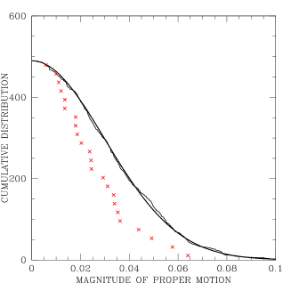
Figure 2.: Cumulative velocity distributions, accumulated from high velocity toward low. In each figure the solid line comes from a lowered Gaussian that corresponds to the potential well at the center of 47 Tuc, while the irregular line is accumulated from the magnitudes of the proper motions of 490 RGB and AGB stars (down to $V$ magnitude 17.0). The left-hand graph shows the whole distribution, while the right-hand graph is a blowup of the region of the cutoff. The crosses in the left-hand graph show the distribution of the motions of blue stragglers, which clearly have a lower velocity dispersion.

Interestingly, we have also been able to examine the “cannonball stars” (Meylan, Dubath, & Mayor 1991) whose existence was part of the original motivation for measuring proper motions in 47 Tucanae. They turn out to have nearly zero proper motions, so that their radial velocities are the whole of their motions, which do not appear to be above the escape velocity at the center of the cluster.

Another distribution that we can examine is that of the blue stragglers. They are known to be more concentrated to the cluster center than are the red giants; they should therefore have a lower velocity dispersion. Their distribution in Fig. 2 confirms this quite well.

2.2. Cluster distances

Although it is outside the immediate focus of this conference, we should mention that the most valuable product of such proper motions will be fundamental distances of globular clusters, found by comparing the dispersion of proper motions, an angular quantity, with that of radial velocities, a linear quantity. With 10,000–20,000 proper motions in a cluster and at least 2500 radial velocities measured by our collaborators (see, e.g., Gebhardt et al. 1997), the only completely unavoidable error will be that due to statistical sample size, which is between 1 and 2%. Our aim, then, will be to avoid all other sources of error. The errors of measurement are not a problem per se; what counts is that their size be accurately known, so that they can be correctly subtracted in quadrature in order to derive the true dispersions.

A serious concern will be the effect of orbital motion in binaries; it must be corrected for statistically, and will be different for the radial velocities and the proper motions, because of the different distribution of the observations in time. To make it worse, the binary fraction in globular clusters is poorly known.

Another problem of consequence takes us back to dynamics: the radial velocities of 47 Tuc stars show a quite prominent rotation of the cluster (Meylan & Mayor 1986). We can in fact see rotation clearly in the proper motions too; at the cluster center they show a slightly greater dispersion in the equatorial than in the polar direction. It is obviously essential that we have a good dynamical model for the cluster. (It should also go without saying that the model should have the correct mass function for this cluster, a precept that has not always been followed. Fortunately our HST observations of the cluster provide a good mass function down to quite low masses.) For the modeling itself we intend to generalize the rotating models of Wilson (1975) to the multi-mass case.

3. The theory of anisotropy in globular clusters

3.1. The origin of anisotropy

The most simple-minded dynamical models of clusters, such as the original “King models” (King 1966), have isotropic velocity distributions, but this is a serious oversimplification for real clusters. Whether a cluster is born by the collapse of a larger configuration or by expansion of a smaller one, the initial motions are largely radial; and conservation of angular momentum in each stellar orbit will then constrain the motions to remain largely radial. This initial anisotropy should be removed gradually as relaxation moves the velocity distribution toward isotropy, and this trend should spread gradually outward from the dense center to the lower-density envelope.

Intuition suggests that the velocity distribution in a cluster should have retained its anisotropy outside the radius where the local relaxation time equals the cluster age (i.e., about a Hubble time), and this is approximately what is observed.

3.2. The nature of anisotropy

In a spherically symmetric globular cluster, the three phase-space variables on which the velocity distribution can depend are the radial distance $r$, the radial component of velocity $v_{{\rm r}}$, and the tangential component of velocity $v_{{\rm t}}$. It has been customary to represent anisotropy in a globular cluster by writing the velocity distribution as

$$f(r,v_{{\rm r}},v_{{\rm t}})=F(E+cJ^{2}),$$ (1)

where

$$E={\textstyle{1\over 2}}\left(v_{{\rm r}}^{2}+v_{{\rm t}}^{2}\right)+U(r)$$ (2)

is the energy per unit mass ($U$ being, of course, the gravitational potential function), and

$$J=rv_{{\rm t}}$$ (3)

is the magnitude of the angular momentum per unit mass. The reasons for this representation are that (1) Jeans’ theorem says that in a time-independent state (which is a very good approximation in a slowly evolving system) the velocity distribution must be a function of these two integrals of the orbital motion of a star, and (2) this simple form is easily shown to lead to a velocity spheroid whose radial elongation increases with increasing $r$.

It is this kind of velocity distribution that Gunn and Griffin (1979) and Meylan (1987, 1988) used in their studies of anisotropy, and a modified form of this distribution that Lupton, Gunn, & Griffin (1987) used in their treatment of anisotropy in a rotating cluster. We will show below, however, that observed anisotropic velocity distributions unfortunately do not have this form.

3.3. Dependence of anisotropy on stellar mass

Nothing is known about how anisotropy differs from one stellar mass to another. We are not aware of any theoretical prediction, nor is there observational information, since existing studies, through radial velocities, have been confined to stars above the main-sequence turnoff, all of which have practically the same mass. We expect to derive such information from observations that will be described below, but for the time being one can only make a rough theoretical estimate.

Anisotropy is removed by relaxation, whose rate goes as $v^{-3}$, where $v$ is a characteristic velocity for the stars in question. Since in the condition of equipartition that seems to exist in nearly all globular clusters $v\propto 1/m$, the time to remove anisotropy would at first appear to go as $m^{-3/2}$. But the dependence on mass should be even stronger, since the stars of lower mass inhabit regions of lower density, on account of their higher velocities, and this makes their relaxation even slower. A quantitative study, however, promises to be rather complicated, and we will not pursue it here.

4. Methods of observing anisotropy

Until now, anisotropy of stellar motions in globular clusters has been studied only indirectly, by comparing the radial drop-off that is observed in the dispersion of radial velocities with the drop-off that is predicted by theoretical models with differing amounts of anisotropy. Not only is this method indirect; it is also too vulnerable to inadequacies in the dynamical modeling. By contrast, proper-motion measurements measure anisotropy directly, and are nearly independent of any modeling.

The analysis of the radial-velocity observations depends on our different geometrical perspective at the center and at the edge of the cluster. The velocities that we observe along the line of sight at the cluster center are clearly values of $v_{{\rm r}}$ only, whereas at points away from the center the observed dispersion has an increasing admixture of $v_{{\rm t}}$, so that the drop-off of ${\langle v^{2}\rangle}_{{\rm los}}$ gives us information about the anisotropy. Unfortunately that information is only indirect. The problem is that there is a natural drop-off of ${\langle v^{2}\rangle}_{{\rm los}}$ even in a cluster whose velocity distribution is isotropic; because the velocity distribution has a cutoff at the escape velocity, the decrease of the latter with increasing radius causes ${\langle v^{2}\rangle}_{{\rm los}}$ to fall. Thus the observed quantity that is needed becomes in effect a higher-order one—the difference between the actual fall-off of ${\langle v^{2}\rangle}_{{\rm los}}$ and the fall-off that would occur in a cluster model that has isotropic velocities. This weakness gives radial velocities only a poor grip on anisotropy. One should note further that such a measurement of anisotropy is very sensitive to the cluster model adopted. The results will suffer badly from any errors either in the assumed mass function or in the functional form that is used for the representation of anisotropy in the velocity distribution. In the latter respect, we will show below that the functional form that has commonly been used is contradicted by our new observations.

The proper motions play a quite different role. At a point away from the cluster center one can directly compare the dispersion in the radial direction with that in the transverse direction. There are, to be sure, projection problems along the line of sight (as there are equally in the interpretation of the radial velocities), but the proper motions give us our only really direct measure of anisotropy.

A caution to note, however, is that rotation of the cluster will distort the apparent anisotropy. Along a given line of sight, components of the rotational motion will be included in the part of the proper motions that is parallel to the cluster equator. (This is similar to the small rotation-induced anisotropy that we have already noted at the cluster center.) Interpretation of the proper motions thus has a small dependence on modeling of the cluster, but far less than in the case of the radial velocities.

5. Our new observations: anisotropy in 47 Tuc

In addition to our work on Meylan’s images at the center of 47 Tucanae, we have a program of our own, in which we have images of two fields on opposite sides of the center of 47 Tuc, each at about 10 core radii from the center. Meylan’s radial-velocity study (1988) suggests that anisotropy becomes strong at a radius somewhere between there and 40 core radii, so our fields should show a modest amount of anisotropy. Our time baselines are 4–5 years. As already indicated, we are able to examine anisotropy directly, by comparing proper-motion dispersions in the radial and transverse directions. We have so far made a preliminary reduction of one of these fields. Although our measurements are still only preliminary, their trend is clear.

The results are surprising. We do see anisotropy, but only among the stars of highest velocity. In other words, in our two-dimensional distribution of proper motions the lines of constant density are not ellipses of constant axial ratio. The contours near the center are circles, while only the largest contours show an elongation in the radial direction. These observations contradict the picture of similar-shaped ellipses that would follow from the sort of velocity distribution that is specified by Eq. (1).

This is a result that we had not foreseen, and as far as we know no one else had either; but it should not have been a surprise, because in clear hindsight it is exactly what we should have expected. To understand it we must keep in mind that anisotropy is removed only by relaxation, whose rate is proportional to the star density in the regions through which a star passes. In a region like the one that we have observed, the stars of low velocity have orbits that bring them into the denser inner regions, where they have seen enough relaxation to isotropize their orbits, whereas those of higher velocity have orbits in which they have spent most of their lives in the low-density outer regions, and with less exposure to the relaxing tendency they have retained some of their anisotropy.

Given the fact that anisotropic velocity distributions are not as we thought they were, how is the theory of cluster dynamics to react? Obviously we need to construct cluster models based on velocity distributions in which the roles of $E$ and $J$ differ from the simplistic ones in Eq. (1). Unfortunately it is not yet clear what sort of mathematical function will fill the bill. An important challenge to the building of realistic dynamical models of star clusters is to find a suitable function. Presumably, for the sake of providing a finite escape velocity it can then be cast in a form analogous to the

$$f(E,J^{2})=e^{-2j^{2}(E+aJ^{2})}-e^{-2j^{2}aJ^{2}},$$ (4)

which is the form used in the now-outmoded models.

We look forward to a better understanding of anisotropy after we have fully reduced the images of these two fields in 47 Tuc, and especially after measuring an outer field in $\omega$ Centauri, where from Meylan’s (1987) results we expect the anisotropy to be much greater.

The interpretation of anisotropy observations will also involve modeling of the cluster. In this case we will need models that include both anisotropy and rotation. Fortunately Lupton & Gunn (1987) have shown how to build such models.

6. Summary

Observations of internal motions in globular clusters are obviously essential for understanding the dynamics of these systems. Radial velocities have contributed some information, but the new ability to measure internal proper motions of individual stars, using the Hubble Space Telescope, opens new vistas for observational studies of dynamics.

Proper motions of large numbers of stars show that the velocity distribution is quite close to Gaussian, as dynamical models have supposed.

Proper motions are much more suitable than radial velocities for the study of anisotropy of velocity dispersions in the outer parts of clusters. Here preliminary results indicate that the anisotropy does not take the form that is customarily assumed in dynamical models; hindsight easily shows why this should be so. New mathematical forms for the velocity distribution need to be contrived.

The most important application of internal proper motions in globular clusters will be the derivation of fundamental distances, from a comparison of the dispersion of the proper motions with that of the radial velocities.

Finally, we note that in a later paper in this volume Ken Freeman reports results of a unique ground-based study that analyzes internal proper motions in $\omega$ Centauri.

Acknowledgments.

The research supported here was supported by grant GO-7503 from the Space Telescope Science Institute.

References

Anderson, J., & King, I. R. 2000, PASP, in press

Gebhardt, K., Pryor, C., Williams, T. B., Hesser, J. E., & Stetson, P. B. 1997, AJ, 113, 1026

Gunn, J. E., & Griffin, R. F. 1979, AJ, 84, 752

King, I. R. 1966, AJ, 71, 66

King, I. R., Anderson, J., Cool, A. M., & Piotto, G. 1998, ApJ, 492, L37

Lupton, R., & Gunn, J. 1987, AJ, 93, 1106

Lupton, R., Gunn, J., & Griffin, R. 1987, AJ, 93, 1114

Meylan, G. 1987, A&A, 184, 144

Meylan, G. 1988, A&A, 191, 215

Meylan, G., & Mayor, M. 1986, A&A, 166, 122

Meylan, G., Dubath, P., & Mayor, M. 1991, ApJ, 383, 587

Wilson, C. P. 1975, AJ, 80, 175