Empirical Determinations of Key Physical Parameters Related to Classical Double Radio Sources

Abstract

Multi-frequency radio observations of the radio bridge of a powerful classical double radio source can be used to determine: the beam power of the jets emanating from the AGN; the total time the source will actively produce jets that power large-scale radio emission; the thermal pressure of the medium in the vicinity of the radio source; and the total mass, including dark matter, of the galaxy or cluster of galaxies traced by the ambient gas that surrounds the radio source. The theoretical constructs that allow a determination of each of these quantities using radio observations are presented and discussed. Empirical determinations of each of these quantities are obtained and analyzed for 22 radio sources; Cygnus A is one of the sources in the sample, but it is NOT used, or needed, to normalize any of these quantities.

A sample of 14 radio galaxies and 8 radio loud quasars with redshifts between zero and two was studied in detail; each source has enough radio information to be able to determine each of the physical parameters listed above. The beam power was determined for each beam of each AGN (so there are two numbers for each source); these AGN are highly symmetric in terms of beam powers. Typical beam powers are about $10^{45}\,\mbox{erg s}^{-1}$. No strong correlation is seen between the beam power and the core - hot spot separation, which suggests that the beam power is roughly constant over the lifetime of a source. The beam power increases with redshift, which is significant after excluding correlations between the radio power and redshift. The relationship between beam power and radio power is not well constrained by the current data.

The characteristic or total time the AGN will actively produce a collimated outflow is estimated. Typical total lifetimes are $\sim(10^{7}$ to $10^{8}$) years. Total source lifetimes decrease with redshift. This decrease in total lifetime with increasing redshift can explain the decrease in the average source size (hot spot - hot spot separation) with redshift. Thus, high-redshift sources are smaller because they have shorter lifetimes; note that higher redshift sources grow more rapidly than low redshift sources.

A new method of estimating the thermal pressure of the ambient gas in the vicinity of a powerful classical double radio source is presented. This new estimate is independent of synchrotron and inverse Compton aging arguments, and depends only upon the properties of the radio lobe and the shape of the radio bridge. A detailed radio map of the radio bridge at a single radio frequency can be used to estimate the thermal pressure of the ambient gas. Thermal pressures on the order of $10^{-10}\,\mbox{dyne cm}^{-2}$, typical of gas in low-redshift clusters of galaxies, are found for the environments of the sources studied here. It is shown that appreciable amounts of cosmic microwave background diminution (the Sunyaev-Zel’dovich effect) are expected from many of these clusters. This could be detected at high frequency where the emission from the radio sources is weak.

The total gravitational mass of the host cluster of galaxies is estimated using the composite pressure profile and the equation of hydrostatic equilibrium for cluster gas. Total masses, and mass-density profiles, similar to those of low-redshift clusters of galaxies are obtained. Thus, some clusters of galaxies, or cores of clusters, exist at redshifts of one to two. The redshift evolution of the cluster mass is not well determined at present. The current data do not indicate any negative evolution of the cluster mass, which may have implications for models of evolution of structure in the universe.

1 Introduction

Classical double radio sources, also known as FRII radio sources (Fanaroff & Riley, 1974), have been extensively studied. Numerous surveys of radio sources as well as detailed studies of individual sources have provided a wealth of radio data on many sources. Theoretical models for the sources developed and discussed by various authors (e.g. Blandford & Rees, 1974; Scheuer, 1974, 1982; Begelman, Blandford, & Rees, 1984; Begelman & Cioffi, 1989; Eilek & Shore 1989; Gopal-Krishna & Wiita 1991; Daly 1990, 2000) lend much understanding to the physics of the sources. It is believed that FRII sources are powered by highly collimated outflows from an active galactic nucleus (AGN), and that the radio emission from these sources is the result of an interaction between the beam, or jet, and the ambient medium. As a result, careful study of FRII sources can yield very useful information about the FRII sources, their environments, and their central engines (e.g. Daly 2000).

Daly (1994, 1995) presents a model for powerful extended FRII sources and showed how key parameters of an FRII source and its environment, such as the beam power and the ambient gas density, can be estimated using multi-frequency radio data. Results for a sample of powerful 3CR radio sources are also presented by the same author (Daly 1994, 1995). A larger sample was compiled and studied in detail; results from these studies have been presented in a series of papers (Wellman & Daly 1996a,b; Wellman 1997; Wellman, Daly, & Wan 1997a, b [hereafter WDW97a,b]; Wan & Daly 1998a,b; Guerra & Daly 1996, 1998; Guerra 1997; Daly, Guerra, & Wan 1998; Guerra, Wan, & Daly 1998; Wan 1998; Daly 2000). For example, detailed results on the density and temperature of the ambient medium of the FRII sources are presented by WDW97a,b, and the redshift evolution of the characteristic size of an FRII source and its application for cosmology are presented by Guerra & Daly (1996, 1998), and Guerra, Daly, & Wan (2000).

This paper presents results on several key parameters of the FRII sources and their environments that were not presented and discussed in previous papers. These parameters include the luminosity in directed kinetic energy of the jet, also known as the beam power, $L_{j}$, the total time the AGN will produce the collimated outflow, $t_{*}$, the thermal pressure of the ambient medium, $P_{th}$, the effect of the hot gas on the microwave background radiation, and the total gravitational mass of the host cluster (we find that the radio sources lie at the centers of gas rich clusters of galaxies). The way that these parameters can be estimated from radio data, and the empirical results for the sample, are presented here.

The paper is structured as follows. A brief description of the sample and data for the sample are presented in §2. Discussions on the jet luminosity and timescale of jet activity are given in §3, the thermal pressure of the ambient medium and estimates of the effect of the hot gas on the microwave background radiation are presented in §4, and estimating the total gravitational mass of the the host cluster of the radio source is discussed in §5. Each of these sections are divided into two subsections, with the first subsection presenting theory and the second one presenting empirical results for the sample. Further discussions of the results and a summary of the paper are presented in §6.

Values of Hubble’s constant $H_{o}=100~{}h~{}\hbox{km s}^{-1}\hbox{Mpc}^{-1}$ and the de/acceleration parameter $q_{o}$=0 (an open empty universe with zero cosmological constant) are used to estimate all the parameters in this study. Different choices of cosmological parameters, within reasonable limits, give results that are very similar to, and consistent with, those presented here.

2 Sample Description and Data

The sample used in this study has been described in detail in several previous papers (e.g. WDW97a,b; Guerra & Daly 1998). The readers are referred to these papers for a full description of the sample; a brief description of it follows. All the FRII sources in this sample are very powerful 3CR sources, having 178 MHz radio power greater than $3\times 10^{26}\hbox{ }h^{-2}\hbox{ W Hz}^{-1}\hbox{sr}^{-1}$; such powerful FRII sources are referred to as FRIIb sources (Daly 2000), or Type 1 FRII sources (Leahy & Williams 1984). They are drawn from the samples of Leahy, Muxlow, & Stephens (1989; hereafter LMS89), which contains sources with large angular sizes, and Liu, Pooley, & Riley (1992; hereafter LPR92), which contains sources with smaller angular extent. The final sample contains 27 radio lobes from 14 FRIIb radio galaxies, and 14 lobes from 8 FRIIb radio loud quasars. These sources have redshifts ranging from zero to 2, and projected core-hot spot separations between $25h^{-1}$ kpc and $200h^{-1}$ kpc. Note that the questions of projection effects and radio power selection effects have been addressed in great detail by Wan & Daly (1998a,b).

WDW97a,b used the radio maps from LMS89 and LPR92 to estimate the width of the radio bridge behind the radio hot spot, $a_{L}$, the non-thermal pressure of the radio lobe that drives the forward shock front, $P_{L}$, and the rate at which the bridge is lengthening, referred to as the lobe propagation velocity $v_{L}$. The radio information may also be used to estimate the beam power and total time the source will be active, as described in §3.

In order to estimate the Mach number of lobe advance, high quality radio maps which image large portions of the radio bridge are required; the radio bridge is defined as the radio emitting region that lies between the radio hot spot and the origin of the host galaxy or quasar. There are 16 bridges in the sample for which we have a detection of the Mach number of lobe advance, which includes 13 radio galaxy bridges and 3 radio loud quasar bridges. The Mach number may be combined with the lobe propagation velocity $v_{L}$ to estimate the temperature of the ambient gas (WDW97a). Thus, the ambient gas temperature and pressure may be estimated for these sources. Lower bounds on the Mach number, and hence upper bounds on the ambient gas temperature and pressure, are available for the 14 other bridges, including 8 galaxy bridges and 6 quasar bridges, as described in WDW97a,b. The maps of the sources do not have sufficient dynamic range to allow detailed analyses of their bridge structure, and thus do not have estimates on the Mach number of lobe advance, nor on the ambient gas pressure and cluster mass. As a result, the sample of sources with estimates of the ambient gas pressure and cluster mass is rather small.

Results for radio-loud quasars and radio galaxies are analyzed separately when there are enough data points, as is the case in the study of the beam power. As noted above, the number of sources with thermal pressure and cluster mass estimates is rather small (16 lobes with detections and 14 with bounds). Thus it is not practical to separate quasars and galaxies in the study of these parameters.

Cygnus A (3C 405) is the only source with a redshift $\sim 0$ in our sample, and in some cases, results seem to depend on whether or not this source is included. Thus, subsamples both with and without Cygnus A are analyzed, and the results included here. Note that Cygnus A is not used to normalize any of the quantities studied here, with the exception of the total source lifetime. Note, however, that an identical normalization of the total source lifetime is obtained when Cygnus A is excluded from the analysis (see the companion paper by Guerra, Daly, & Wan 2000). Thus, Cygnus A is not needed to normalize any of the quantities studied here.

3 Luminosity in Directed Kinetic Energy of the Jet

3.1 Theory

The jet or beam of an FRII radio source refers to the collimated outflow which carries energy from the AGN. When the jet impinges upon the external medium, a strong shock is formed and the kinetic energy of the jet is deposited in the vicinity of the shock front, which is marked by the radio hot spot. In principle, one can calculate the beam power, $dE/dt$, carried by the jet by studying the propagation of the hot spots. However, in practice it is difficult to use hot spot properties to estimate the beam power, since the hot spot is generally not resolved, and the position and properties of radio hot spots vary on short time scales (Laing 1989; Carilli, Perley, and Dreher 1988; Black et al. 1992.).

The model presented and discussed by (Daly 1994, 1995) bypasses these difficulties by using properties of the more stable radio lobes to estimate the luminosity in directed kinetic energy, or the beam power, $L_{j}$. This model is a natural progression following the work of Blandford & Rees (1974), Scheuer (1974), Eilek & Shore (1989), Gopal-Krishna & Wiita (1991), Rawlings & Saunders (1991), and many others. The method and results presented here are complementary to those of Eilek & Shore (1989) in the sense that Eilek & Shore (1989) considered the case of a non-supersonic expansion of the radio emitting region, while we consider the supersonic expansion of this region, and the shape of the radio emitting region considered here is different from that considered by Eilek & Shore. The results presented here are also complementary to those of Gopal-Krishna & Wiita (1991), who consider likely explanations for the decrease in FRII radio source size with redshift, and who present a consistent picture in which the increase in radio luminosity and decrease in radio source size with redshift can be understood. The work presented here differs from that of Gopal-Krishna & Wiita (1991) in that neither an efficiency nor an evolution of the ambient gas density with redshift are adopted. Instead, we use the radio properties of a source to solve directly for the beam power of the source, as well as several other parameters, including the ambient gas density. The work presented here on the beam power is similar in spirit to that of Rawlings & Saunders (1991). The key difference is that here the radio bridge is assumed to be cylindrically symmetric, and thus has a volume that depends on the length of the bridge times the cross-sectional area of the bridge, while Rawlings & Saunders (1991) seem to take a bridge volume that is proportional to the cube of the bridge length.

Observations and numerical simulations indicate that radio lobes of powerful extended radio sources propagate supersonically relative to the ambient medium (Alexander & Leahy 1987; Prestage & Peacock 1988; Cox, Gull, & Scheuer 1991; Daly 1994; WDW97a,b). Leahy (1990) shows that the properties of the radio lobe can be used to estimate the rate of energy input. In §3.4.4.3, Leahy (1990) shows that the jet power may be written $(3P+P)V/\tau$, since the energy density of a relativistic plasma is 3 times the pressure P; note that the time rate of change of the volume may be written: $V/\tau=\pi a_{L}^{2}~{}v_{L}$ since the forward region of the source grows with a velocity $v_{L}$ and has cross-sectional area $\pi a_{L}^{2}$. His equation may be rewritten as:

$$L_{j}=4\pi a_{L}^{2}v_{L}P_{L}.$$ (1)

Here $a_{L}$ is the cross-sectional radius of the radio lobe, $v_{L}$ is the lobe propagation velocity, and the FRII source is assumed to be cylindrically symmetric about the radio axis. Using typical units, $L_{j}$ can be expressed as

$$L_{j}=3.6\times 10^{44}\mbox{erg s}^{-1}\left({a_{L}\over\mbox{kpc}}\right)^{2}\left({v_{L}\over c}\right)\left({P_{L}\over 10^{-10}\,\mbox{dyne cm}^{-2}}\right),$$ (2)

All three parameters used to estimate $L_{j}$ in eq. (2) can be estimated from radio data (see, for example, Daly 1995, or WDW97a,b). The lobe radius $a_{L}$ can be measured from the radio map (see WDW97a,b for detail). The lobe propagation velocity $v_{L}$ can be estimated using multi-frequency observations of radio lobes and bridges, by modeling the spectral aging of relativistic electrons due to synchrotron and inverse Compton losses (cf. WDW97a,b; Wan & Daly 1998a,b; Myers & Spangler 1985; Alexander & Leahy 1987; LMS89; LPR92; Carilli et al. 1991; Perley & Taylor 1991). The lobe pressure $P_{L}$ is given by

$$P_{L}=\left(\frac{4}{3}b^{-1.5}+b^{2}\right){B_{min}^{2}\over 24\pi},$$ (3)

where $B_{min}$ is the magnetic field strength in the radio lobe under the minimum-energy condition (cf. Miley 1980; Pacholczyk 1970), $b$ is the ratio of the true magnetic field strength $B$ to the minimum-energy magnetic field strength: $B=bB_{min}$, and the equation is in cgs units. WDW97b estimate $b$ to be about 0.25, with a source-to-source dispersion less than about $15\%$. This value of $b$ is consistent with values obtained by other authors (cf. Carilli et al. 1991; Perley & Taylor 1991; Feigelson et al. 1995), and is used throughout this study.

The radio spectral index of an FRII source is used in the spectral aging analysis to estimate the lobe propagation velocity $v_{L}$. It is shown in WDW97b that there is a clear correlation between the radio spectral indices of the sources in this sample and redshift. The spectral index $\alpha$ can be expressed as $\alpha\propto(1+z)^{s}$. The best fitted value of $s$ is $0.8\pm 0.2$ with a reduced $\chi^{2}$ of 1.7. Such a correlation could be caused by intrinsic curvature in the initial electron energy spectrum or effects of inverse Compton cooling on the hot spot spectral index (see WDW97b). Thus, the observed spectral index may not be the appropriate index to used in spectral aging analysis. This lead WDW97b to also consider correcting the observed spectral indices to zero redshift using the empirical correlation between $\alpha$ and $(1+z)$ for the sample. Results obtained with and without this correction are included here.

The beam power $L_{j}$ can be used to estimate the total time that the AGN will be active, and will produce highly collimated outflows. Following Daly (1994, 1995) and Guerra & Daly (1996, 1998), the total lifetime of an outflow, defined as $t_{\star}$, is related to the energy extraction rate $L_{j}$ by a power law:

$$t_{\star}=CL_{j}^{-\beta_{\star}/3},$$ (4)

where $\beta_{\star}$ is a parameter that has implications for models of energy extraction from the central engine. As described in detail in a companion paper (see Guerra, Daly, & Wan 2000), eq. (4) is equivalent to assuming that the source will have an average size close to the average size of the full population located at a similar redshift, and that the average rate of growth of the source will be close to the current rate of growth of the source. Thus, we could have written $t_{*}\simeq<D>/v_{L}$ where $<D>$ is the average size of the full population of FRIIb sources at similar redshift, and $v_{L}$ is the rate of growth of the source under consideration. Since this is precisely the manner in which the value of $\beta_{*}$ is obtained, it is an equivalent approach. Note that the value of $\beta_{*}$ is, fortuitously, independent of choice of cosmological parameters, and it is independent of the way the relation is normalized (see the companion paper of Guerra, Daly, & Wan 2000).

The current best estimate of $\beta_{\star}$ is $1.75\pm 0.25$ (see the compansion paper of Guerra, Daly, & Wan 2000). (Note that the $\beta_{\star}$ used here is not related to $\beta_{0}$ used in §4 and §5 for the King density profile.) The characteristic size of an FRII source is related to its lifetime as $D_{\star}=v_{L}t_{\star}=Cv_{L}L_{j}^{-\beta_{*}/3}$, where $C$ is the normalization in eq. (4). This normalization factor is chosen so that at $z\approx 0$, the characteristic size of Cygnus A matches the observed average lobe-lobe size for sources at this redshift. That is, $(v_{L})CL_{j}^{-\beta_{*}/3}$ for one side of Cygnus A is added to $(v_{L})CL_{j}^{-\beta_{*}/3}$ on the other side of Cygnus A, and this is set equal to $2(<D>_{z=0})$ = $2\times(68\pm 14)$ kpc. This equation is then solved for the normalization factor $C$; the uncertainty on $C$ is indicated in Table 1. This normalization is then used in equation (4) to obtain an estimate of the total time that the AGN will be producing large-scale jets. Note that a nearly identical normalization is obtained when Cygnus A is excluded from the data analysis, as shown in a compansion paper (Guerra, Daly, & Wan 2000). Note also that the constraints on $\beta$ and on cosmological parameters are independent of this normalization, as described in Guerra, Daly, & Wan (2000). The value for $t_{*}$ estimated using independent information from each side of the source should of course be equal, and are generally very close in value. The value adopted for the beam power, $L_{j}$, of Cygnus A used above is listed in Table 1, $v_{L}$ for Cygnus A is obtained from Table 1 from WDW97b, and a value of $<D>_{z=0}$ = $(68\pm 14)$ kpc is adopted from Table 3 of Guerra, Daly, & Wan (2000).

The results on $t_{*}$ do not depend on the normalization adopted here; as shown in a companion paper, nearly identical results obtain when Cygnus A is excluded from the analysis. And, Cygnus A is not used to normalize any other quantity. Thus, none of the results presented in this paper rely upon a normalization based on Cygnus A.

3.2 Empirical Results

The beam power, $L_{j}$, has been estimated using eq. (2) for the lobe propagation velocity estimated using the observed radio spectral index, and the redshift-corrected radio spectral index; both are listed in Table 1. Typical values of $L_{j}$ are $10^{45}\,\mbox{$h^{-2}$ erg s}^{-1}$.

No strong correlation is found between the beam power $L_{j}$ and the linear size of the source, represented by the core-hot spot separation $r$. Figure 1 is a log-log plot of $L_{j}$ vs. $r$, where the observed radio spectral index $\alpha$ is used. The figure of $L_{j}$ vs. $r$ after applying the redshift-correction on $\alpha$ is almost identical to Figure 1, and is thus not shown here.

For radio-loud quasars, the best-fitted line in Fig. 1 has a slope of about zero. A Spearman rank correlation analysis shows that the correlation coefficient between $L_{j}$ and $r$ is $-0.03(7.72\%)$ when no redshift-correction on the spectral index is applied, and $-0.01(1.78\%)$ when the spectral index correction is applied. Here the number in parentheses is the significance of the correlation. These results suggest that the correlation between $L_{j}$ and $r$ for radio-loud quasars is insignificant, either with or without the $\alpha\!-\!z$ correction. That is, $L_{j}$ is independent of $r$ for the radio-loud quasars.

For radio galaxies, $L_{j}$ appears to increase slightly with $r$ in Fig. 1, and results from the Spearman rank correlation analysis hint a marginally significant correlation between $L_{j}$ and $r$. The correlation coefficient is about 0.3, with a significance level of about $90\%$, which holds with or without the $\alpha\!-\!z$ correction. However, note that the best-fitted line for radio galaxies in Fig. 1 has a slope only $2\sigma$ away from zero, and that a correlation coefficient of about 0.3 is rather weak. Thus it appears that $L_{j}$ is at most weakly dependent on $r$ for radio galaxies. These results for radio-loud quasars and radio galaxies are consistent with the assumption that $L_{j}$ is roughly constant over a source’s lifetime.

The relationship between $L_{j}$ and redshift and radio power ($P_{r}$) has been studied in detail in Wan & Daly (1998a). Increases of $L_{j}$ with $z$ and with $P_{r}$ are observed (see Figures 2 and 3). However, the radio power of the sources in the sample also increases with redshift since the sources used in this study all come from the flux-limited 3CR survey. As a result, which of the $L_{j}-z$ and $L_{j}-P_{r}$ correlations is more significant, and the role of radio power selection effects, needs to be considered carefully. Wan & Daly (1998a) used two parameter fitting and partial rank analysis to investigate this. The two parameter fit $L_{j}\propto P_{178}^{n_{p}}(1+z)^{n_{z}}$ yields the following $n_{z}$ values: $n_{z}=1.45\pm 0.32(0.60)$ for all galaxies, $n_{z}=3.83\pm 0.93(1.73)$ for all galaxies except for Cygnus A, and $n_{z}=9.56\pm 1.37(3.91)$ for all radio-loud quasars.

The number in parenthesis is the uncertainty on $n_{z}$ times $\sqrt{\chi_{r}^{2}}$, which includes the effect of a reduced $\chi^{2}$ $(\chi_{r}^{2})$ that is greater than one for the fit. This notation will be used throughout this paper.

The values of $n_{z}$ are more that $2\sigma$ away from zero, for both radio galaxies and radio-loud quasars. This means that the $L_{j}-z$ correlation is unlikely to be caused purely by radio power selection effects. That is, a real increase of $L_{j}$ with redshift exists, though the magnitude of this redshift evolution is not well determined.

The $L_{j}-P_{r}$ correlation, on the other hand, is rather poorly constrained. Results from the one parameter fit suggest $L_{j}$ goes roughly proportional to $P_{178}$ (Figure 3). The two parameter fit $L_{j}\propto P_{178}^{n_{p}}(1+z)^{n_{z}}$, which takes into account the redshift dependence of radio power, gives values of $n_{p}$ with large uncertainties: $n_{p}=0.76\pm 0.11(0.20)$ for all galaxies, $n_{p}=0.25\pm 0.22(0.41)$ for all galaxies except for Cygnus A, and $n_{p}=-0.54\pm 0.29(0.82)$ for all radio-loud quasars. Thus, the exact relationship between $L_{j}$ and radio power is not clear at the present time. Note, however, large amounts of scatter are seen in the $L_{j}$ vs. $P_{178}$ plot (see Figure 3), which is also reflected in the large reduced $\chi^{2}$ of the one parameter fit. For the same beam power, the radio power can vary by about a factor of ten. This suggests that radio power is not an accurate measure of the beam power, and that the apparent correlation between $L_{j}$ and $P_{r}$ may result from the fact that both increase with redshift.

The properties of FRIIb radio sources suggest that the total lifetime of a source decreases systematically with redshift. This follows because the average size of FRIIb sources decreases with redshift, while the rate of growth of the sources increases with redshift. Another way to state this is: as $L_{j}$ increases with redshift, the total lifetime of an outflow, $t_{\star}$, estimated using eq. (4), decreases with redshift. The values of the full lifetime of the source $t_{\star}$ are listed in Table 1. Typical values of $t_{\star}$ range from about $10^{7}$ to $10^{8}$ years. Figure 4 plots $t_{\star}$ as a function of redshift. It is clear that $t_{\star}$ decreases with $z$, which can explain the fact that the average size of powerful extended 3CR sources decreases with redshift for $z>0.3$ (see Guerra & Daly 1998), while the lobe propagation velocity $v_{L}$ increases with redshift. Clearly if $v_{L}$ increases with redshift, and the mean source size $D_{*}$ decreases with redshift, then $t_{*}$ must decrease with redshift since $D_{*}\simeq v_{L}t_{*}$. The sources at high redshift produces more powerful jets (with larger $L_{j}$) for a shorter period of time (with smaller $t_{*}$), which results in smaller average sizes than low-redshift sources.

4 Thermal Pressure of the Ambient Gas

4.1 Theory

The studies of WDW97a and b show that both the ambient gas density and temperature of an FRIIb source can be estimated from radio data. The thermal pressure of the ambient gas $P_{th}$ is obviously proportional to the product of the density $n_{a}$ and the temperature $T$. Interestingly, as shown below, although the lobe propagation velocity enters into $n_{a}$ and $T$, it cancels out in the product, so the thermal pressure of the ambient gas can be estimated using single frequency radio data if the radio emission from the bridge is mapped over a large enough region of the bridge. This offers a completely new method to estimate the thermal pressure of the ambient gas surrounding high-redshift radio sources using only single frequency radio data.

It can be complicated and time consuming to estimate the ambient gas density in the vicinity of classical double radio sources using X-ray observations, especially for sources at high redshift. An attractive alternative method of estimating $n_{a}$ in the vicinity of a radio source is to use the radio data. Given that the radio lobe represents a strong shock front, the lobe pressure $P_{L}$, the ambient gas density $\rho_{a}$, and the lobe propagation velocity are related: the strong shock jump conditions imply that $P_{L}\approx 0.75\rho_{a}v_{L}^{2}$ holds, where $P_{L}$ is the non-thermal pressure inside the radio lobe, and $\rho_{a}$ is the mass density of the ambient gas. The electron number density of the ambient gas $n_{a}$ can be estimated using

$$n_{a}\simeq{P_{L}\over 1.4\mu m_{p}v_{L}^{2}},$$ (5)

where $\mu$ is the mean molecular weight of the gas in AMU, with a value of 0.63 when solar abundances are assumed, and $m_{p}$ is the proton mass.

The ambient gas temperature can be estimated by careful studies of the radio bridge, as discussed in detail in WDW97a. A brief description of the theory is as follows. When the non-thermal pressure of the radio bridge is much greater than the ambient gas pressure, the bridge undergoes supersonic expansion. This lateral expansion can be treated as a blast wave and the expansion velocity is determined by ram pressure confinement. This causes the width of the bridge, $a$, to vary with time approximately as $t^{1/2}$ (e.g. Begelman & Cioffi 1989; Daly 1990; WDW97a). Since the lobe propagation velocity $v_{L}$ is roughly constant during a given source’s lifetime (e.g. LPR92; WDW97a,b), the lobe front will advance a distance of $v_{L}t$ during $t$ as the bridge expands. This means that at a distance $x$ from the hot spot, the bridge expansion time is $t=x/v_{L}$. Thus the shape of the radio bridge roughly follows a square root law, with the bridge width $a(x)\propto x^{1/2}$. This behavior was in fact found by WDW97a. As the bridge expands, the pressure inside decreases until it becomes comparable to the ambient gas pressure. When this occurs, the lateral expansion velocity becomes sonic, causing a break in the functional form of $a(x)$. The width of the bridge starts to deviate from the square root law and becomes roughly constant as equilibrium is being reached. At the point where such a break occurs, the lateral expansion velocity is approximately sonic. Thus the sound speed of the ambient gas ($c_{s}$) can be estimated using

$$c_{s}\approx\left.v_{s}\right|_{b}=\left.{da\over dt}\right|_{b}=\left.{da\over dx}\right|_{b}{dx\over dt}=\left.{da\over dx}\right|_{b}\cdot v_{L},$$ (6)

where $\left.v_{s}\right|_{b}$ denotes the lateral expansion velocity at the break.

The Mach number of lobe propagation is defined as $M\equiv v_{L}/c_{s}$. Given the expression for $c_{s}$ in eq. (6), the Mach number of lobe propagation is:

$$M\equiv{v_{L}\over c_{s}}\approx\left(\left.{da\over dx}\right|_{b}\right)^{-1}={2x_{b}\over a_{b}},$$ (7)

where $a_{b}$ is the width of the bridge at the break, and $x_{b}$ is the position of the break relative to the hot spot (see WDW97a). It can be seen from eq. (7) that $M$ depends only on the geometrical shape of the radio bridge.

The ambient gas temperature T can be expressed as:

$$T={\mu m_{p}\over\gamma k}c_{s}^{2}\propto\left(\left.{da\over dx}\right|_{b}\right)^{2}\cdot v_{L}^{2}\propto v_{L}^{2}M^{-2},$$ (8)

where $\gamma$ is the ratio of specific heats of the ambient gas.

Multi-frequency radio maps are required in order to use eqs. (5) and (8) to estimate the ambient gas density and temperature of an FRII source, since both $n_{a}$ and $T$ depend on $v_{L}$. The product $n_{a}~{}T$ is independent of $v_{L}$, so $v_{L}$ is not needed to estimate the thermal pressure of the ambient gas. The ambient gas pressure in the vicinity of the radio lobe is simply

$$P_{th}=(n_{a}+n_{i})kT\propto\left({P_{L}\over v_{L}^{2}}\right)v_{L}^{2}M^{-2}\propto{P_{L}\over M^{2}},$$ (9)

with $P_{L}$ estimated using eq. (3) and $M$ estimated using eq. (7). Here $n_{i}$ is the number densities of ions, and for a gas with solar abundances, the electron density is $n_{a}=1.21n_{i}$. Substituting in the numerical constants in eqs. (5) and (8), the thermal pressure is given by

$$P_{th}=0.8{P_{L}\over M^{2}},$$ (10)

for a gas with a specific heat ratio $\gamma=5/3$.

The thermal pressure estimated using eq. (10) depends only on the lobe pressure $P_{L}$ and the geometrically determined Mach number $M$, both of which can be obtained from single frequency observations of the radio lobe and bridge. No spectral aging analysis is needed in order to estimate $P_{th}$, since the dependences of $n_{a}$ and $T$ on $v_{L}$ cancel. As a result, $P_{th}$ is also independent of whether or not the redshift-correction on the radio spectral index is applied.

At low-redshift, X-ray data can often be used to estimate $n_{a}$ and $T$, and hence $P_{th}$. However, high-resolution X-ray data are often difficult to obtain for sources at high redshift. This new method of estimating $P_{th}$, using single frequency radio data, offers an attractive alternative. It provides a powerful tool to study the environments of powerful classical double radio sources, especially those at high-redshift. Since it has been shown that these sources are in cluster-like gaseous environments, the sources may be used to study evolution of gas in clusters of galaxies (as discussed by Daly 1995; WDW97a,b; Daly 2000).

4.2 Empirical Results

The value of $P_{th}$, the thermal pressure of the ambient gas in the vicinity of the radio lobe, is listed in Table 1. Most sources in the sample have $P_{th}$ on the order of ($10^{-11}$ to $10^{-10})\,h^{4/7}\,\mbox{dyne cm}^{-2}$, which is typical of gas in low-redshift clusters of galaxies. This is consistent with results obtained by WDW97(a,b), who find cluster-like density and temperature for the ambient gas of the FRII sources in the sample. Note that the thermal pressures obtained here do not depend on a spectral aging analysis, whereas density and temperature estimates do.

The X-cluster around Cygnus has been observed by Arnaud et. al. (1984) and Carilli, Perley, & Harris (1994). The thermal pressure of the ambient gas near its radio lobe is estimated to be about $10^{-10}\,\mbox{dyne cm}^{-2}$ (see Carilli, Perley, & Harris 1994). This estimate from X-ray data is consistent with the thermal pressure estimated here for Cygnus A (3C 405) using the new method just described (see Table 1).

The composite pressure profile, $P_{th}$ as a function of the core-hot spot separation $r$, is shown in Figure 5. It can be seen that $P_{th}$ decreases with $r$. A negative pressure gradient is expected for an isothermal gas distribution that follows the King density profile, which is suggested to be the ambient gas distribution for sources in our sample (WDW97a,b). For this gas distribution, the thermal pressure decreases with $r$ as

$$P_{th}(r)=P_{th,\,c}\left[1+\left({r\over r_{c}}\right)^{2}\right]^{-{3\over 2}\beta_{0}},$$ (11)

where $P_{th,\,c}$ is the thermal pressure at the center of the cluster, and $r_{c}$ is cluster core radius.

The pressure gradient seen Figure 5 appears to be consistent with that expected for an cluster gas distribution that is isothermal and follows a King density profile, with a cluster core radius $r_{c}$ of $\sim(50\mbox{ to }150)\,h^{-1}$ kpc. The sources in our sample have values of $r$ ranging from (25 to 250) $h^{-1}$ kpc. Within this radius range, the pressure profile given by eq. (11) has an average slope of ($\sim\!-1.4\mbox{ to }-0.7$), for $r_{c}$ values of (50 to $150\,h^{-1}$ kpc), assuming $\beta_{0}=2/3$. These expected slopes are consistent with the best-fit slopes of $\sim\!-1.0\pm 0.3$ in Figure 5.

There is some hint of a redshift evolution of the cluster core radius from the data. Figure 6 plots $P_{th}$ vs. $r$ in two redshift bins, $z\!<\!0.9$ and $z\!>\!0.9$. The division at $z=0.9$ is chosen so that the two redshift bins cover about the same range in redshift and contain about the same number of data points. It appears that $P_{th}$ decreases less rapidly with $r$ at high redshift than at low redshift, suggesting a larger $r_{c}$ at high redshift. The best-fit slope of $\sim\!-1.4$ in the low-redshift bin is consistent with $r_{c}\sim 50\,h^{-1}$ kpc for the pressure profile given by eq. (11), whereas the best-fit slope of about $-0.4$ in the high-redshift bin is consistent with $r_{c}\sim 250\,h^{-1}$ kpc. This result is still preliminary since only sources with detections of $P_{th}$ are included in the fits. Better estimates of $P_{th}$ for sources currently with only upper bounds on $P_{th}$ will help to better determine whether $r_{c}$ is evolving with redshift.

The results obtained above are consistent with results obtained by WDW97b. They study the ambient gas density profile and find that $r_{c}\sim 50\,h^{-1}$ kpc when high- and low-redshift source are considered together. They also find that that data are consistent with a constant core gas mass model where $r_{c}$ increases with redshift roughly as $r_{c}\propto(1+z)^{1.6}$. Note that results from the study of $P_{th}$ do not depend on spectral aging analysis, whereas those from the study of $n_{a}$ do. It is thus encouraging that consistent results are obtained from the two studies.

For the following analysis, we use both a non-evolving core radius of $50\,h^{-1}$ kpc, and an evolving core radius of $50\,(1+z)^{1.6}h^{-1}$ kpc, with a focus on the latter.

The thermal pressure at the center of the cluster ($P_{th,\,c}$) can be estimated by scaling the pressure in the vicinity of the radio lobe ($P_{th}$) to the cluster center. This follows because the studies of Daly (1995) and WDW97a,b indicate that these radio sources are located at the centers of clusters of galaxies, so the core-hot spot separation can be used as an estimate of distance from the cluster center. The current data on $T$, $n_{a}$, and $P_{th}$ are all consistent with the gas distribution being isothermal and following a King profile. Thus we use the pressure profile for such a gas distribution, as given by eq. (11), to estimate the central thermal pressure. The central pressure is simply

$$P_{th,\,c}=P_{th}(r)\left[1+\left({r\over r_{c}}\right)^{2}\right]^{{3\over 2}\beta_{0}},$$ (12)

The values of $P_{th,\,c}$ for the sources in our sample are listed in Table 1, where a value of $\beta_{0}=2/3$ has been assumed. Most sources have values of $P_{th,\,c}$ around $10^{-10}\,h^{4/7}\,\mbox{dyne cm}^{-2}$, which is rather typical of gas pressure in the core regions of low-redshift galaxies clusters.

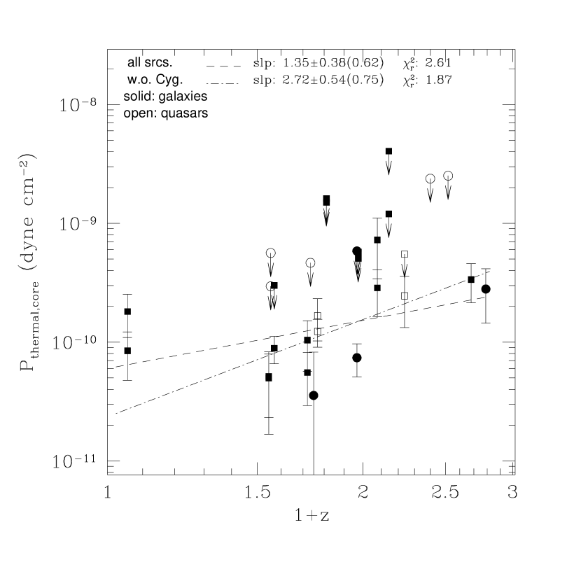
Figure 7: Thermal pressure of the ambient gas at the cluster center vs. redshift for an isothermal gas distribution that follows the King density profile. A non-evolving cluster radius of $50h^{-1}$ kpc, and $\beta_{0}=2/3$ are used. The same plots for an evolving core radius of $50(1+z)^{1.6}h^{-1}$ kpc are very similar to these and are not shown here. Bounds are not included in the fits.

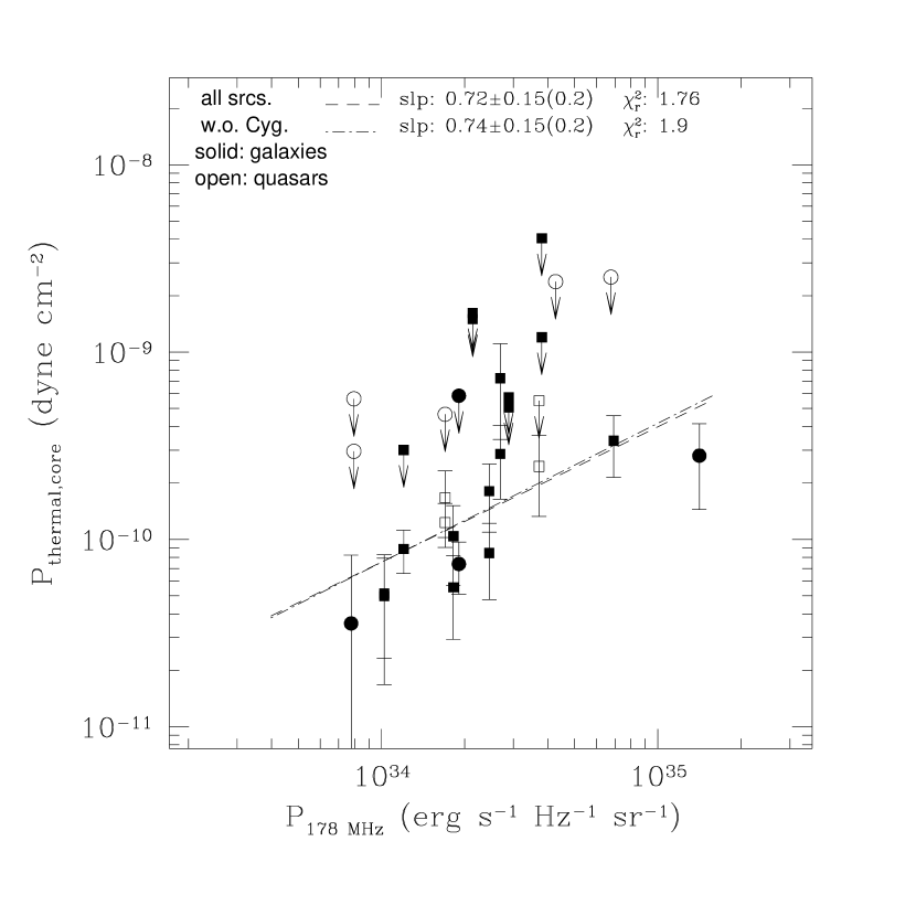
Figure 8: Thermal pressure of the ambient gas at the cluster center vs. the radio power at 178 MHz for an isothermal gas distribution that follows the King density profile. A non-evolving cluster radius of $50h^{-1}$ kpc, and $\beta_{0}=2/3$ are used. The same plots for an evolving core radius of $50(1+z)^{1.6}h^{-1}$ kpc are very similar to these and are not shown here. Bounds are not included in the fits.

Results on the redshift evolution of the central gas pressure $P_{th,\,c}$ are somewhat uncertain because $P_{th,\,c}$ seems to correlate with both redshift and radio power when either correlation is considered separately (see Figures 7 and 8), and it is not clear at present which correlation is more significant. For the non-evolving core radius model, a two-parameter fit of $P_{th,\,c}\propto(1+z)^{n_{z}}P_{178}^{n_{p}}$ yields $n_{z}=0.29\pm 0.49(0.67)$ and $n_{p}=0.66\pm 0.19(0.26)$ when all sources are included, and $n_{z}=1.51\pm 2.11(2.99)$ and $n_{p}=0.34\pm 0.58(0.82)$ when Cygnus A is not included. For the evolving core radius model, the two-parameter fit gives $n_{z}=-1.22\pm 0.49(0.65)$ and $n_{p}=0.88\pm 0.19(0.25)$ when all sources are included, and $n_{z}=1.56\pm 2.11(2.82)$ and $n_{p}=0.15\pm 0.58(0.78)$ when Cygnus A is not included. Note that Cygnus A appears to lie in a cooling-flow region while most of the other sources are not in cooling-flow regions (see WDW97a; §5). Thus fits with and without Cygnus A are both performed. In any case, the large uncertainties on $n_{z}$ and $n_{p}$ make it hard to determine the magnitude of the redshift evolution of $P_{th,\,c}$.

The thermal pressure can be used to predict the amount of cosmic microwave background (CMB) diminution, also known as the Sunyaev-Zel’dovich (S-Z) effect, that is expected from the cluster. The reduction in the cosmic radiation ($\Delta I_{\nu}$) in the direction of a cluster is given by (e.g. Sunyaev & Zel’dovich 1980; Sarazin 1988; Rephaeli 1995)

$$\Delta I_{\nu}/I_{\nu}=G(\omega)y.$$ (13)

Here $I_{\nu}$ is the specific intensity of the CMB at the observing frequency $\nu$, $y$ is the Comptonization parameter, and the function $G(\omega)$ is

$$G(\omega)={\omega e^{\omega}\over e^{\omega}-1}\left[\omega\left({e^{\omega}+1\over e^{\omega}-1}\right)-4\right],$$ (14)

where $\omega\equiv h\nu/kT_{r}$, and $T_{r}=2.73\,\mbox{K}$ is the CMB temperature (Mather et al. 1990).

The Compton $y$ parameter is given by

$$y=\int{kT\over m_{e}c^{2}}\sigma_{T}n_{e}dl={\sigma_{T}\over m_{e}c^{2}}\left({n_{e}\over n_{e}+n_{i}}\right)\int P_{th}dl.$$ (15)

where $\sigma_{T}=(8\pi/3)[e^{2}/(m_{e}c^{2})]^{2}$ is the Thompson electron scattering cross section, $T$ is the cluster gas temperature, $n_{e}$ is the electron density, and $n_{i}$ is the ion density. Using the thermal pressure in a cluster with an isothermal-King gas distribution (eq. [11]), this gives

$$y\approx 6.3\times 10^{-5}\left({\mbox{\raisebox{4.0pt}{$P_{th,\,c}$} }\over\mbox{\raisebox{-4.0pt}{$10^{-10}$\,dyne cm${}^{-2}$} }}\right)\left({\mbox{\raisebox{4.0pt}{$r_{c}$ }}\over\mbox{\raisebox{-4.0pt}{0.25\,Mpc}}}\right){\mbox{\raisebox{4.0pt}{$\Gamma(3\beta_{0}/2-1/2)$ }}\over\mbox{\raisebox{-4.0pt}{$\Gamma(3\beta_{0}/2)$ }}}\,(1+x^{2})^{-3\beta_{0}/2+1/2},$$ (16a)

where $$x\equiv r/r_{c} n_{e}=1.21n_{i} \beta_{0}=2/3$$, and the gas is taken to have solar abundance so that . For a typical value of ,

$$y\approx 1.12\times 10^{-4}\left({P_{th,\,c}\over 10^{-10}\,\mbox{dyne cm}^{-2}}\right)\left({r_{c}\over 0.25\,\mbox{Mpc}}\right)(1+x^{2})^{-1/2}.$$ (16b)

At low frequency, clusters with strong radio sources are generally avoided for measurements of the Sunyaev-Zel’dovich effect because emission from the radio source masks the microwave diminution. Such contaminations from radio sources are reduced at high frequency since emission from steep-spectrum radio sources, such as the FRII sources studied here, decreases rapidly with increasing frequency. The Sunyaev-Zel’dovich Infrared Experiment (SuZIE) can measure the S-Z effect around 140 GHz, where the amount of CMB intensity diminution is near its peak. At this frequency, a cluster with an isothermal-King density profile will cause a CMB intensity diminution of about

$$\begin{array}[]{ll}\Delta I_{\nu}\approx 7.0\times 10^{-19}\mbox{erg s${}^{-1}$Hz${}^{-1}$cm${}^{-2}$sr${}^{-1}$ }\left({\mbox{\raisebox{4.0pt}{$P_{th,\,c}$} }\over\mbox{\raisebox{-4.0pt}{$10^{-10}$\,dyne cm${}^{-2}$} }}\right)\left({\mbox{\raisebox{4.0pt}{$r_{c}$ }}\over\mbox{\raisebox{-4.0pt}{0.25\,Mpc}}}\right)\\ \times{\mbox{\raisebox{4.0pt}{$\Gamma(3\beta_{0}/2-1/2)$ }}\over\mbox{\raisebox{-4.0pt}{$\Gamma(3\beta_{0}/2)$ }}}\,(1+x^{2})^{-3\beta_{0}/2+1/2},\end{array}$$ (17)

and for a typical value of $\beta_{0}=2/3$,

$$\Delta I_{\nu}\approx 1.24\times 10^{-18}\mbox{erg s${}^{-1}$Hz${}^{-1}$cm${}^{-2}$sr${}^{-1}$ }\left({P_{th,\,c}\over 10^{-10}\,\mbox{dyne cm}^{-2}}\right)\left({r_{c}\over 0.25\,\mbox{Mpc}}\right)(1+x^{2})^{-1/2}.$$ (18)

For a detector with a FWHM beam size $\theta_{b}$, the total amount of CMB diminution within the beam, defined as $\Delta F_{\nu}$, is roughly

$$\Delta F_{\nu}\approx f\cdot 24\,\mbox{mJy}\left({\theta_{b}\over\mbox{1.7 arcmin}}\right)^{2}\left({P_{th,\,c}\over 10^{-10}\,\mbox{dyne cm}^{-2}}\right)\left({r_{c}\over 0.25\,\mbox{Mpc}}\right),$$ (19)

where $f$ is the beam dilution factor, defined as the ratio of the average $\Delta I_{\nu}$ within the beam to the peak value at the cluster center; and the SuZIE FWHM beam size at 140 GHz of 1.7 arcmin (e.g. Holzapfel et al. 1997) is used to calculate the numerical value. For a Gaussian beam, when the HWHM beam size corresponds to 1$r_{c}$, $f\approx 0.7$, and when the HWHM beam size corresponds to 2$r_{c}$, $f\approx 0.5$ (see Rephaeli 1987). At $z<2$, the SuZIE beam radius is less than $\sim 320\,h^{-1}\mbox{kpc}$ for $q_{0}=0$ with no cosmological constant. Thus a cluster with $P_{th,\,c}\!\sim\!10^{-10}\,\mbox{dyne cm}^{-2}$ and $r_{c}\!\sim\,0.25\,\mbox{Mpc}$ will have a $\Delta F_{\nu}$ of about (15 to 20) mJy within the SuZIE beam. The clusters surrounding the FRII sources in our sample have $P_{th,\,c}$ on the order of $10^{-10}\,h^{4/7}\,\mbox{dyne cm}^{-2}$ and the data also suggest that $r_{c}$ increases with redshift, reaching about $300\,h^{-1}\,\mbox{kpc}$ at $z\!\sim\!2$. The expected CMB diminution within the SuZIE beam at 140 GHz for these clusters ranges from several to tens of mJy. These clusters make good candidates for SuZIE observations if the fluxes from the radio sources at 140 GHz or their uncertainties are small compared with the expected S-Z effect signals.

We are currently in the process of searching for high frequency data on the radio sources in our sample in oder to identify possible SuZIE observation candidates. One likely candidate that comes from a preliminary search in the published literature is 3C239. The expected CMB diminution for the cluster surrounding it is about $30\,h^{-3/7}$ mJy within the SuZIE beam at 140 GHz. In contrast, extrapolation of the observed spectrum of 3C239 as given by observations at 178 MHz, 10.7 GHz, and 14.9 GHz (Kellermann & Pauliny-Toth 1973; Genzel et al. 1976; Laing, Riley, and Longair 1983), gives a 140 GHz flux of only 6 mJy. This is likely to be an overestimate since synchrotron aging and inverse Compton cooling can both cause the high frequency spectral index to become steeper than that at low frequency. The effects of inverse Compton cooling can be especially important since this source is at high redshift ($z=1.79$), where the energy density of the microwave background is much higher than at low redshift. Thus it appears that emission from this radio source is weak compared with the expected CMB diminution. Observations of the radio source at more frequencies above 14.9 GHz can help to better constrain its 140 GHz flux.

5 Gravitational Mass of the Host Cluster

5.1 Theory

The powerful classical double radio sources studied here are in cluster-like gaseous environments (see WDW97a, b). The studies of these sources provide information on density and temperature of the ambient gas. Thus it is possible to estimate one of the most important parameters of the cluster, the total gravitational mass, including dark matter.

The total mass can be estimated using the density and temperature profile of the intracluster medium (ICM) if the gas is in hydrostatic equilibrium. The sound crossing time in the ICM is usually short compared to the age of a high-redshift cluster, and the morphology of the X-ray emission from many low-redshift clusters is often smooth. Thus it is generally believed that hydrostatic equilibrium is a good approximation of the state of the ICM for many clusters that are not cooling flow clusters. Assuming spherical symmetry, hydrostatic equilibrium requires

$${1\over\rho_{g}}{dP\over dr}=-{GM_{t}(r)\over r^{2}},$$ (20)

where $\rho_{g}$ is the gas density and $M_{t}(r)$ is the total gravitating mass within $r$. This means that

$$M_{t}(r)=-{kT(r)\over G\mu m_{p}}\cdot r\cdot\left[{d\log\rho_{g}(r)\over d\log r}+{d\log T(r)\over d\log r}\right],$$ (21)

where $k$ is the Boltzman constant, $\mu$ is the mean molecular weight of the gas in amu, $m_{p}$ is the proton mass, and $T(r)$ and $\rho_{g}(r)$ are the temperature and density profiles of the cluster gas.

The most commonly used hydrostatic model of the ICM is the isothermal $\beta$-model (Cavaliere & Fusco-Femiano, 1976,1978; Sarazin & Bahcall 1977), where the clusters gas is isothermal and the density profile follows a modified King model, i.e., $n_{a}=n_{c}[1+(r/r_{c})^{2}]^{-3/2\beta_{0}}$. Here $n_{c}$ is the core density and $r_{c}$ is core radius of the gas distribution. Using this model for the ICM, eq. (21) becomes

$$M_{t}(r)={3\beta_{0}k\over G\mu m_{p}}\cdot T\cdot r\cdot{(r/r_{c})^{2}\over 1+(r/r_{c})^{2}}.$$ (22)

Results from numerical simulations of cluster formation suggest that departures of the ICM from hydrostatic equilibrium are usually small, and the mass estimated using the standard $\beta$-model is rather accurate (e.g. Navarro, Frenk & White 1995; Schindler 1996; Evrard, Metzler, & Navarro 1996). Note however, significant temperature decline is observed to occur at outer regions of clusters (e.g. Markevitch et al. 1998). Thus, we only use eq. (22) to estimate the cluster mass within $r$ rather than extrapolating to large radii.

The mass estimated using eq. (22) is not accurate if the cluster is cooling at the point where the cluster temperature is measured. Inside a cooling flow region, the temperature measured does not indicate the gravitational potential, since hydrostatic equilibrium conditions do not apply. Considering cooling only by thermal bremsstrahlung, which dominates other mechanisms at typical cluster temperatures, the cooling time of the cluster gas can be estimated using

$$t_{cool}\approx 2.1\times 10^{-2}\left({T\over 10^{7}\,\mbox{K}}\right)^{1/2}\left({n_{a}\over\mbox{cm}^{-3}}\right)^{-1}\mbox{Gyr},$$ (23)

where $T$ and $n_{a}$ are the ambient gas temperature and electron density, respectively (see WDW97a). Note this equation does not depend on the Hubble’s constant, provided that the estimates of $n_{a}$ and $T$ do not depend on Hubble’s constant.

Given the ambient gas temperature and density estimates, the cooling time for the sources in our sample can be estimated (see WDW97a). A cooling time less than the age of the universe at that redshift means that the FRII source is in a cooling flow region. To estimate the age of the universe at a given redshift, an open empty universe is assumed, with a current age of 14 Gyr, which corresponds to $h\approx 0.7$ for $q_{0}=0$ with zero cosmological constant.

Most sources in our sample do not appear to be cooling at the position where the temperature is measured. Thus their mass estimates are likely to be reliable. A few sources, including the low-redshift source Cygnus A, appear to lie in cooling flow regions.

Figure 9 shows the total cluster mass, including dark matter, within radius $r$, $M_{t}(r)$, as a function of the core-hot spot separation $r$. Since the sources appear to lie at the centers of clusters of galaxies (Daly 1995; WDW97a,b), the core-hot spot separation is used to estimate the distance from the cluster center. The radio spectral index is redshift-corrected, and the cluster core radius is taken to be $r_{c}=50(1+z)^{1.6}\,h^{-1}$ kpc (see §4.2). Clusters that are cooling at the position where the temperature is measured are marked with pentagons. The plots of $M_{t}(r)$ vs. $r$ for other models, either with or without an $\alpha\!-\!z$ correction and/or different core radius evolution, are presented in Figures 10 through 12.

The cluster mass increases with $r$ for all models. The increase is more rapid for models with an evolving core radius than models with a fixed core radius. This merely reflects the fact that with an increasing $r_{c}$, more sources lie within the core region, where the increase of mass with radius is rapid, and varies roughly as $M\propto r^{3}$.

To determine the redshift evolution of the cluster mass, a three parameter fit of $M_{t}(r)\propto r^{n_{1}}(1+z)^{n_{2}}P_{178}^{n_{3}}$ is performed since the cluster mass within $r$, $M_{t}(r)$, is a function of $r$, and may also be affected by radio power selection effects. Results are listed in Table 2 for all models considered. A two parameter fit of $M_{t}(r)\propto r^{n_{1}}(1+z)^{n_{2}}$ is also performed, and results are listed in Table 3. For completeness, fits including all sources, all sources except Cygnus A, and all sources that are not in cooling flow regions, are all listed in the table. Note that Cygnus A appears to be in a cooling flow region for all the models considered. Results obtained excluding cooling flow clusters are probably the correct ones to consider.

The sample of clusters with mass estimates is rather small, especially when only non-cooling flow clusters are considered. Thus it is not surprising to see that the best-fit values of $n_{2}$ have rather large uncertainties, which makes it hard to draw definitive conclusions about the redshift evolution of the cluster mass. Note though, the current data do not indicate any negative evolution of the cluster mass out to a redshift of about two. This is consistent with results obtained by this group (Daly 1994; Guerra & Daly 1996, 1998; Guerra, Daly, & Wan 2000; and Daly, Guerra, & Wan 1998), who study the characteristic size of powerful classical double radio sources and find the data suggest a low value of $\Omega_{m}$; a universe with $\Omega_{m}=1$ is ruled out at 99 % confidence (see Guerra, Daly, & Wan 2000).

There are some indications from the data that the redshift evolution of the cluster core radius, and the redshift-correction on the radio spectral index are favored. The gas mass within $r$, defined as $M_{g}(r)$, can be estimated using

$$M_{g}(r)=4\pi\rho_{c}r_{c}^{3}[x-\mbox{tan}^{-1}(x)],$$ (24)

where $\rho_{c}$ is the central gas density, $r_{c}$ is the core radius, $x\equiv r/r_{c}$, and a typical value of $\beta_{0}=2/3$ is used for the King density profile. Knowing the gas mass and the total mass within $r$, the gas mass fraction within $r$ can be estimated. The gas mass fraction within radius $r$ as a function of redshift is shown in Figure 13, where the radio spectral index is redshift-corrected and the core radius is taken to be $r_{c}=50(1+z)^{1.6}\,h^{-1}$ kpc.

The values of gas fraction shown in the figure are consistent with observed values for inner regions of many clusters (e.g. Donahue 1996), whereas those for models without a redshift-correction on the radio spectral index, and without a core radius evolution seem to be low compared with observed values.

Several factors may contribute to the slow decrease of gas fraction with redshift that is seen in Figure 13. First, the increase of cluster core radius with redshift means that the gas fraction estimated for the high-redshift clusters is over a larger fraction of the cluster core than for the low-redshift clusters. The gas fraction estimated at high redshift mainly represents the gas fraction inside the cluster core, and it is known that gas fraction increases with increasing radius in clusters (e.g. David, Jones, & Forman 1995). Second, the mass contribution from galaxies is higher at the cluster center than at large radii (e.g. Loewenstein & Mushotzky 1996). Thus by sampling a larger fraction of the cluster core at higher redshift, a larger fraction of the total baryon mass is not taken into account at higher redshift. Further, the decrease in gas fraction with redshift could be due to the stripping of gas from galaxies in the cluster core over time. Finally, the cluster gas becomes more concentrated toward the cluster center as it cools, which also causes the gas fraction in the cluster center to increase with time.

These results on cluster mass and gas fraction obtained above are still preliminary due to the small size of the sample. More sources with estimates on the ambient gas temperature, and hence cluster mass, will help to test these results.

6 Summary and Discussion

Several key parameters of an FRII source and its gaseous environment are studied in this paper.

Direct estimates of the beam power, which measures the energy extraction rate from the AGN by the jet, are obtained. Typical beam powers of about $10^{45}\,h^{-2}\,\mbox{erg s}^{-1}$ are found for the sources in the sample. No strong correlation is seen between the beam power and the linear size of the source, which is consistent with the beam power being roughly constant throughout the lifetime of a source.

There is a trend for the beam power to increase with redshift, which is significant even after excluding radio power selection effects. The magnitude of this redshift evolution, however, is not well determined by the current data. It is well known that the quasar luminosity function undergoes strong evolution between $z\!\sim\!0$ and $z\!\sim\!2$, with the high-redshift quasars being more luminous than their low-redshift counterparts (e.g. Schmidt & Green 1983; Yee & Ellingson 1993; La Franca & Cristiani 1997). This suggests that high-redshift AGNs are more powerful than low redshift ones. Thus it is perhaps not surprising to find that the beam power, or energy per unit time channeled into the jet by the AGN, is also higher at high redshift.

The relationship between the beam power and the radio power is not well constrained after their correlations with redshift are taken into account. The two parameter fit of $L_{j}\propto(1+z)^{n_{z}}P_{178}^{n_{p}}$ yields values of $n_{p}$ with large uncertainties. Thus it is not clear at present how the beam power and the radio power are related. However, the large amount of scatter seen in the beam power-radio power relation suggests that radio power is not an accurate measure of beam power.

The beam power $L_{j}$ can be used to estimate the total lifetime of an outflow produced by an AGN. Following Daly (1994) and Guerra & Daly (1996, 1998), the total time for which the outflow will occur, $t_{\star}$, is related to $L_{j}$: $t_{\star}\propto L_{j}^{-\beta_{\star}/3}$, where $\beta_{\star}$ is estimated to be about $1.75\pm 0.25$ (Guerra, Daly, & Wan 2000). Typical lifetimes of about $10^{7}$ to $10^{8}$ years are obtained for the sources studied here. This would is almost precisely the same lifetime as would be obtained by dividing the average size of all FRIIb sources at similar redshift by the rate of growth of the source under consideration. The lifetime of the outflow decreases with redshift, which explains the decrease of the average size of powerful extended 3CR sources with redshift. The sources at high redshift produces more powerful jets for a shorter period of time, which results in smaller average sizes than low-redshift sources.

A new method of estimating the thermal pressure of the ambient gas in the vicinity of powerful classical double radio source using only single frequency radio data is presented. The pressure is given by the product of the ambient gas density, estimated using ram pressure confinement of the radio lobe, and the ambient gas temperature, estimated using the Mach number for the source and the lobe advance speed. It turns out that the lobe propagation velocity cancels out of the product $n_{a}T$, and the ambient gas pressure can be estimated by studying the shape of the radio bridge, and the non-thermal pressure of the radio lobe (see §4). Thus, the thermal pressure, the product of the ambient gas density and temperature, depends only on the non-thermal pressure in the radio lobe and the geometrically determined Mach number of lobe advance, both of which can be estimated using single frequency radio data. This new method to estimate the thermal pressure does not require a spectral aging analysis, and provides a powerful tool to probe the environments of FRII sources. The thermal pressure estimated for Cygnus A using this new method agrees with that obtained using X-ray data (see §4.2.).

Thermal pressures on the order of $10^{-10}\,h^{4/7}\,\mbox{dyne cm}^{-2}$, typical of gas in low-redshift clusters of galaxies, are found for the gaseous environments of the FRII sources studied here. There are hints from the current data that the gradient of the composite pressure profile is less steep at high redshift than at low redshift, which can be explained by an increase of the cluster core radius with redshift. The current data are consistent with a core radius evolution from $\sim\!50\,h^{-1}\,\mbox{kpc}$ at $z\!\sim\!0$ to $\sim\!250\,h^{-1}\,\mbox{kpc}$ at $z\!\sim\!2$, which agrees with results obtained from studies of the ambient gas density (WDW97b). WDW97b find that the data can be described by a model where the core gas density decreases and the core radius increases so that the core gas mass remains roughly constant.

The thermal pressures obtained here can be used to estimate the amount of CMB diminution expected from the clusters surrounding the FRII sources in the sample. Contaminations from the radio sources can be reduced by observing at high frequency, such as 140 GHz, since emission from the radio sources decreases rapidly with increasing frequency. The cluster surrounding a source in our sample can be detected by SuZIE observations at 140 GHz if the flux from the radio source at this frequency or its uncertainty is small compared with the expected S-Z effect signal. A search for high-frequency data of the sources in our sample is ongoing in oder to identify possible SuZIE observation candidates. Preliminary results suggest that 3C239 is a good candidate.

The gravitational or total mass of the surrounding cluster is estimated for the sources in the sample, assuming hydrostatic equilibrium conditions for the gas. Masses of up to $10^{14}M_{\odot}$ are found for the central regions ($r\lesssim 250\,h^{-1}\,\mbox{kpc}$) of the clusters, consistent with typical values for low-redshift clusters. The redshift evolution of the cluster mass is not well determined. Current data do not indicate negative evolution of the cluster mass. This is consistent with results obtained by members of this group (Guerra & Daly 1996, 1998; Guerra, Daly, & Wan 2000; Daly, Guerra, & Wan 1998), who study the characteristic size of FRII sources and find the data strongly favor a low value for the density parameter $\Omega_{m}$; a universe with $\Omega_{m}=1$ is ruled out at 99 % confidence. Note, however, that with the study presented here, we only study the central regions of clusters.

The values of gas mass fraction obtained for the clusters surrounding the FRII sources studied here are consistent with observed values for central regions of clusters, after the correlation between the radio spectral index and redshift is taken into account, and a redshift evolution of the cluster core radius is considered. This suggests that the cluster core radius evolution and the effects of the radio spectral index-redshift correlation are important.

The gas mass fraction seems to decrease slowly with redshift. The increase of cluster core radius with redshift can be one cause. Another possible explanation is that a large fraction of the gas is still in the galaxies at high redshift, and is later stripped from the galaxies into the cluster at low redshift. Cooling of the cluster gas also tends to cause the gas mass fraction in the cluster center to increase with time.

The results on mass and gas fraction should be taken as preliminary because of the small size of the sample.

Table 1: Source Properties

Source		z	Log$L_{j}$(I)	Log$L_{j}$(II)	Log$P_{th}$	Log$P_{th,c}(A)$	Log$P_{th,c}(B)$	$t_{\star}$(I)	$t_{\star}$(II)
3C 55	G	0.72	$45.55\pm 0.15$	$45.39\pm 0.15$	$-11.34\pm 0.19$	$-10.26\pm 0.19$	$-10.87\pm 0.19$	$1.8\pm 0.3$	$2.2\pm 0.4$
			$45.49\pm 0.18$	$45.33\pm 0.18$	$-11.08\pm 0.19$	$-9.98\pm 0.19$	$-10.60\pm 0.19$	$1.9\pm 0.5$	$2.3\pm 0.6$
3C 68.1	Q	1.238	$46.11\pm 0.12$	$45.88\pm 0.12$	$-10.50\pm 0.19$	$-9.61\pm 0.19$	$-10.32\pm 0.19$	$0.8\pm 0.1$	$1.1\pm 0.2$
			$45.53\pm 0.15$	$45.28\pm 0.14$	$<-10.25$	$<-9.26$	$<-10.03$	$1.8\pm 0.3$	$2.5\pm 0.4$
3C 68.2	G	1.575	$45.53\pm 0.30$	$45.25\pm 0.29$	$\cdots$	$\cdots$	$\cdots$	$1.8\pm 0.7$	$2.6\pm 1.0$
			$45.73\pm 0.17$	$45.48\pm 0.17$	$\cdots$	$\cdots$	$\cdots$	$1.4\pm 0.3$	$1.9\pm 0.4$
3C 154	Q	0.58	$44.30\pm 0.12$	$44.17\pm 0.12$	$\cdots$	$\cdots$	$\cdots$	$9.4\pm 1.3$	$11.1\pm 1.5$
			$44.65\pm 0.12$	$44.51\pm 0.12$	$\cdots$	$\cdots$	$\cdots$	$5.9\pm 0.9$	$7.0\pm 1.0$
3C 175	Q	0.768	$45.18\pm 0.11$	$45.02\pm 0.11$	$-10.50\pm 0.15$	$-9.78\pm 0.15$	$-10.27\pm 0.15$	$2.9\pm 0.4$	$3.5\pm 0.4$
			$45.57\pm 0.11$	$45.41\pm 0.11$	$-10.85\pm 0.09$	$-9.91\pm 0.09$	$-10.50\pm 0.09$	$1.7\pm 0.2$	$2.1\pm 0.3$
3C 239	G	1.79	$46.16\pm 0.13$	$45.87\pm 0.12$	$-9.80\pm 0.20$	$-9.55\pm 0.20$	$-9.79\pm 0.20$	$0.8\pm 0.1$	$1.1\pm 0.2$
3C 247	G	0.749	$44.99\pm 0.15$	$44.83\pm 0.15$	$-10.54\pm 0.57$	$-10.45\pm 0.57$	$-10.53\pm 0.57$	$3.7\pm 0.8$	$4.6\pm 0.9$
			$44.69\pm 0.16$	$44.54\pm 0.16$	$\cdots$	$\cdots$	$\cdots$	$5.5\pm 1.2$	$6.8\pm 1.4$
3C 254	Q	0.734	$44.97\pm 0.13$	$44.80\pm 0.12$	$<-9.54$	$<-9.33$	$<-9.50$	$3.8\pm 0.6$	$4.8\pm 0.7$
3C 265	G	0.811	$44.97\pm 0.19$	$44.80\pm 0.19$	$<-9.97$	$<-8.79$	$<-9.48$	$3.8\pm 1.0$	$4.7\pm 1.2$
			$45.26\pm 0.19$	$45.10\pm 0.19$	$<-9.86$	$<-8.82$	$<-9.47$	$2.6\pm 0.6$	$3.2\pm 0.8$
3C 267	G	1.144	$45.58\pm 0.19$	$45.36\pm 0.19$	$<-9.16$	$<-8.39$	$<-9.01$	$1.7\pm 0.4$	$2.2\pm 0.6$
			$45.58\pm 0.14$	$45.38\pm 0.14$	$<-9.64$	$<-8.92$	$<-9.51$	$1.7\pm 0.3$	$2.2\pm 0.4$
3C 268.1	G	0.974	$45.32\pm 0.13$	$45.18\pm 0.13$	$<-10.17$	$<-9.30$	$<-9.93$	$2.4\pm 0.4$	$2.9\pm 0.5$
			$45.66\pm 0.12$	$45.55\pm 0.12$	$<-10.00$	$<-9.24$	$<-9.81$	$1.5\pm 0.2$	$1.7\pm 0.3$
3C 268.4	Q	1.4	$45.99\pm 0.22$	$45.72\pm 0.21$	$<-8.79$	$<-8.62$	$<-8.77$	$1.0\pm 0.3$	$1.4\pm 0.4$
3C 270.1	Q	1.519	$45.96\pm 0.19$	$45.64\pm 0.18$	$\cdots$	$\cdots$	$\cdots$	$1.0\pm 0.3$	$1.5\pm 0.4$
			$45.96\pm 0.14$	$45.71\pm 0.14$	$<-8.76$	$<-8.60$	$<-8.75$	$1.0\pm 0.2$	$1.4\pm 0.3$
3C 275.1	Q	0.557	$43.95\pm 0.17$	$43.80\pm 0.17$	$<-9.75$	$<-9.53$	$<-9.69$	$15.0\pm 3.4$	$18.1\pm 4.0$
			$44.61\pm 0.14$	$44.47\pm 0.14$	$<-9.36$	$<-9.25$	$<-9.33$	$6.2\pm 1.2$	$7.4\pm 1.4$
3C 280	G	0.996	$45.29\pm 0.13$	$45.11\pm 0.13$	$\cdots$	$\cdots$	$\cdots$	$2.5\pm 0.4$	$3.1\pm 0.5$
			$44.98\pm 0.11$	$44.79\pm 0.11$	$\cdots$	$\cdots$	$\cdots$	$3.8\pm 0.5$	$4.8\pm 0.6$
3C 289	G	0.967	$45.15\pm 0.11$	$44.96\pm 0.11$	$-10.25\pm 0.12$	$-10.13\pm 0.12$	$-10.24\pm 0.12$	$3.0\pm 0.4$	$3.8\pm 0.5$
			$45.18\pm 0.12$	$45.00\pm 0.12$	$<-9.35$	$<-9.23$	$<-9.33$	$2.9\pm 0.4$	$3.6\pm 0.5$
3C 322	G	1.681	$46.11\pm 0.20$	$45.79\pm 0.19$	$\cdots$	$\cdots$	$\cdots$	$0.8\pm 0.2$	$1.3\pm 0.3$
			$46.14\pm 0.12$	$45.88\pm 0.12$	$-10.08\pm 0.14$	$-9.47\pm 0.14$	$-10.03\pm 0.14$	$0.8\pm 0.1$	$1.1\pm 0.2$
3C 330	G	0.549	$45.24\pm 0.18$	$45.16\pm 0.18$	$-11.19\pm 0.23$	$-10.29\pm 0.23$	$-10.76\pm 0.23$	$2.7\pm 0.6$	$2.9\pm 0.7$
			$45.15\pm 0.15$	$45.02\pm 0.14$	$-11.18\pm 0.28$	$-10.30\pm 0.28$	$-10.76\pm 0.28$	$3.0\pm 0.6$	$3.5\pm 0.7$
3C 334	Q	0.555	$44.94\pm 0.12$	$44.81\pm 0.12$	$\cdots$	$\cdots$	$\cdots$	$4.0\pm 0.5$	$4.7\pm 0.6$
			$45.05\pm 0.22$	$44.89\pm 0.20$	$\cdots$	$\cdots$	$\cdots$	$3.4\pm 0.9$	$4.2\pm 1.1$
3C 356	G	1.079	$45.62\pm 0.21$	$45.41\pm 0.21$	$-10.51\pm 0.22$	$-9.14\pm 0.22$	$-10.01\pm 0.22$	$1.6\pm 0.4$	$2.1\pm 0.6$
			$45.88\pm 0.21$	$45.69\pm 0.21$	$-10.59\pm 0.17$	$-9.54\pm 0.17$	$-10.29\pm 0.17$	$1.1\pm 0.3$	$1.4\pm 0.4$
3C 405	G	0.056	$45.07\pm 0.13$	$45.06\pm 0.13$	$-10.31\pm 0.19$	$-10.07\pm 0.19$	$-10.10\pm 0.19$	$3.3\pm 0.6$	$3.4\pm 0.6$
			$44.99\pm 0.12$	$44.97\pm 0.12$	$-10.04\pm 0.17$	$-9.74\pm 0.17$	$-9.78\pm 0.17$	$3.7\pm 0.6$	$3.8\pm 0.6$
3C 427.1	G	0.572	$44.72\pm 0.13$	$44.60\pm 0.13$	$<-9.81$	$<-9.52$	$<-9.72$	$5.3\pm 0.9$	$6.2\pm 1.0$
			$44.83\pm 0.11$	$44.71\pm 0.11$	$-10.37\pm 0.09$	$-10.05\pm 0.09$	$-10.27\pm 0.09$	$4.6\pm 0.6$	$5.4\pm 0.7$

Table 2: Results Obtained by Fitting $M_{t}(r)\propto r^{n_{1}}(1+z)^{n_{2}}P_{178}^{n_{3}}$

type	No.	$\alpha$-$z$?	$r_{c}$-$z$?	$n_{1}$	$n_{2}$	$n_{3}$	$\chi_{r}^{2}$
N.C.Cl.	11	Yes	Yes	2.38 $\pm$ 0.70(0.52)	6.86 $\pm$ 5.48(4.1)	-1.31 $\pm$ 1.57(1.17)	0.56
G+Q-C	14	Yes	Yes	2.95 $\pm$ 0.31(0.23)	2.72 $\pm$ 3.80(2.84)	-0.08 $\pm$ 1.01(0.76)	0.56
G+Q	16	Yes	Yes	2.88 $\pm$ 0.30(0.23)	-0.73 $\pm$ 0.96(0.73)	0.80 $\pm$ 0.37(0.28)	0.58
N.C.Cl.	13	No	Yes	3.05 $\pm$ 0.36(0.28)	4.46 $\pm$ 4.11(3.18)	-0.13 $\pm$ 1.06(0.82)	0.60
G+Q-C	14	No	Yes	2.95 $\pm$ 0.31(0.23)	3.66 $\pm$ 3.82(2.88)	0.02 $\pm$ 1.02(0.77)	0.57
G+Q	16	No	Yes	2.89 $\pm$ 0.30(0.23)	0.49 $\pm$ 0.96(0.73)	0.83 $\pm$ 0.37(0.28)	0.58
N.C.Cl.	11	Yes	No	1.36 $\pm$ 0.63(0.52)	7.40 $\pm$ 4.55(3.72)	-0.93 $\pm$ 1.33(1.09)	0.67
G+Q-C	14	Yes	No	2.12 $\pm$ 0.27(0.23)	3.18 $\pm$ 3.33(2.85)	0.44 $\pm$ 0.90(0.77)	0.73
G+Q	16	Yes	No	2.11 $\pm$ 0.26(0.21)	1.63 $\pm$ 0.91(0.75)	0.84 $\pm$ 0.33(0.27)	0.68
N.C.Cl.	13	No	No	2.17 $\pm$ 0.31(0.28)	4.45 $\pm$ 3.40(3.10)	0.47 $\pm$ 0.88(0.80)	0.83
G+Q-C	14	No	No	2.12 $\pm$ 0.27(0.23)	4.09 $\pm$ 3.20(2.77)	0.53 $\pm$ 0.86(0.74)	0.75
G+Q	16	No	No	2.11 $\pm$ 0.27(0.22)	2.84 $\pm$ 0.91(0.76)	0.86 $\pm$ 0.33(0.27)	0.69

Table 3: Results Obtained by Fitting $M_{t}(r)\propto r^{n_{1}}(1+z)^{n_{2}}$

type	No.	$\alpha$-$z$?	$r_{c}$-$z$?	$n_{1}$	$n_{2}$	$\chi_{r}^{2}$
N.C.Cl.	11	Yes	Yes	2.70 $\pm$ 0.59(0.45)	2.39 $\pm$ 1.24(0.94)	0.58
G+Q-C	14	Yes	Yes	2.95 $\pm$ 0.31(0.22)	2.43 $\pm$ 1.05(0.75)	0.51
G+Q	16	Yes	Yes	2.67 $\pm$ 0.29(0.28)	0.63 $\pm$ 0.73(0.69)	0.90
N.C.Cl.	13	No	Yes	3.04 $\pm$ 0.35(0.26)	3.99 $\pm$ 1.16(0.86)	0.55
G+Q-C	14	No	Yes	2.95 $\pm$ 0.31(0.22)	3.74 $\pm$ 1.06(0.76)	0.52
G+Q	16	No	Yes	2.67 $\pm$ 0.29(0.28)	1.90 $\pm$ 0.73(0.70)	0.93
N.C.Cl.	11	Yes	No	1.60 $\pm$ 0.52(0.42)	4.30 $\pm$ 1.04(0.84)	0.65
G+Q-C	14	Yes	No	2.13 $\pm$ 0.27(0.22)	4.75 $\pm$ 0.83(0.68)	0.68
G+Q	16	Yes	No	1.88 $\pm$ 0.25(0.27)	3.34 $\pm$ 0.62(0.66)	1.13
N.C.Cl.	13	No	No	2.20 $\pm$ 0.31(0.27)	6.19 $\pm$ 0.94(0.82)	0.77
G+Q-C	14	No	No	2.13 $\pm$ 0.27(0.23)	6.00 $\pm$ 0.83(0.70)	0.72
G+Q	16	No	No	1.88 $\pm$ 0.25(0.27)	4.57 $\pm$ 0.62(0.67)	1.16

Figure 1: The luminosity in directed kinetic energy of the jet vs. the core-hot spot separation. The best-fitted lines for all galaxies, all galaxies except Cygnus A, and all radio-loud quasars, are shown with a solid line, a dashed line and a dotted line, respectively. Slopes of the best-fitted lines are labeled. The number in parenthesis is the uncertainty on the slope times $\sqrt{\chi_{r}^{2}}$, which includes the effect of a reduced $\chi^{2}$, defined as $\chi_{r}^{2}$, greater than one for the fit.

Figure 2: The luminosity in directed kinetic energy of the jet vs. redshift.

Figure 3: The luminosity in directed kinetic energy of the jet vs. the radio power at 178 MHz.

Figure 4: Total lifetime of the collimated outflows vs. redshift.

Figure 5: Thermal pressure of the ambient gas in the vicinity of the radio lobe vs. the core-hot spot separation. The best-fitted lines for all sources, including galaxies and quasars, and all sources except Cygnus A are shown with a dashed line and a dash-dot line, respectively. Only sources with detections of the Mach number $M$, and hence $P_{th}$, are included in the fit.

Figure 6: Thermal pressure of the ambient gas in the vicinity of the radio lobe vs. the core-hot spot separation for two redshift bins ($z<0.9$, $z>0.9$). In the low-redshift bin, slopes of the best-fitted lines are $-1.43\pm 0.21(0.27)$ with a reduced $\chi^{2}$ of 1.58 for all sources, and $-1.35\pm 0.25(0.32)$ with a reduced $\chi^{2}$ of 1.65 for all sources except Cygnus A. In the high redshift bin, the slope of the best-fitted line is $-0.41\pm 0.20(0.30)$ with a reduced $\chi^{2}$ of 2.29. Only sources with detections of $P_{th}$ are included in the fit.

Figure 9: Cluster mass within $r$ vs. the core-hot spot separation $r$. An isothermal gas distribution that follows the King density profile with an evolving cluster core radius of $50\,(1+z)^{1.6}h^{-1}$ kpc and $\beta_{0}=2/3$ is used. The radio spectral index is redshift-corrected. Sources that are cooling at the point where the cluster temperature $T$ is measured are marked with pentagons. The best-fitted lines for all sources, including both galaxies and quasars, all sources except Cygnus A, and all sources that are not cooling, are shown with a dashed line, a dot-dash line, and a solid line, respectively. Only sources with detections of $T$, hence mass, are included in the fit.

Figure 10: Cluster mass within $r$ vs. the core-hot spot separation $r$. An isothermal gas distribution that follows the King density profile with an evolving cluster core radius of $50\,(1+z)^{1.6}h^{-1}$ kpc and $\beta_{0}=2/3$ is used. The radio spectral index is not redshift-corrected.

Figure 11: Cluster mass within $r$ vs. the core-hot spot separation $r$. An isothermal gas distribution that follows the King density profile with a fixed cluster core radius of $50\,h^{-1}$ kpc and $\beta_{0}=2/3$ is used. The radio spectral index is redshift-corrected.

Figure 12: Cluster mass within $r$ vs. the core-hot spot separation $r$. An isothermal gas distribution that follows the King density profile with a fixed cluster core radius of $50\,h^{-1}$ kpc and $\beta_{0}=2/3$ is used. The radio spectral index is not redshift-corrected.

Figure 13: Gas fraction ($M_{gas}/M_{t}$) within radius $r$ vs. redshift. The radio spectral index is redshift-corrected, and an isothermal gas distribution that follows the King density profile with an evolving cluster core radius of $50\,(1+z)^{1.6}h^{-1}$ kpc and $\beta_{0}=2/3$ is used.

References

- Alexander & Leahy (1987) Alexander, P., & Leahy, J. P. 1987, 255, 1
- Arnaud et. al. (1984) Arnaud, K. A., Fabian, A. C., Eales, S. A., Jones, C., & Forman, W. 1984, MNRAS, 211, 981
- Begelman, Blandford, & Rees (1984) Begelman, M. C., Blandford, R. D., & Rees, M. J. 1984, Rev. Mod. Phys., 56, 255
- Begelman & Cioffi (1989) Begelman, M. C., & Cioffi, D. F., 1989, ApJ, 345, L21
- (5) Black, A. R. S., Baum, S. A., Leahy, J. P., Perley, R. A., Riley, J. M., & Scheuer, P. A. G. 1992, MNRAS, 256, 186
- Blandford & Rees (1974) Blandford, R. D., & Rees, M. J. 1974, MNRAS, 169, 395
- Carilli, Perley, & Dreher (1988) Carilli, C. L., Perley, R. A., & Dreher, J. H. 1988, ApJ, L73
- Carilli et al. (1991) Carilli, C. L., Perley, R. A., Dreher, J. W., & Leahy, J. P., 1991, ApJ, 383, 554
- Carilli, Perley, & Harris (1994) Carilli, C. L., Perley, R. A., & Harris, D. E. 1994, MNRAS, 270, 173
- Cavaliere & Fusco-Femiano (1976) Cavaliere, A., & Fusco-Femiano, R. 1976, A&A, 49, 137
- Cavaliere & Fusco-Femiano (1978) Cavaliere, A., & Fusco-Femiano, R. 1978, A&A, 70, 677
- Cox, Gull, & Scheuer (1991) Cox, C. I., Gull, S. F., & Scheuer, P. A. 1991, MNRAS, 252, 558
- (13) David, L. P., Jones, C., & Forman, W. 1995, ApJ, 445, 578
- Daly (1990) Daly, R. A. 1990, ApJ, 355, 416
- Daly (1994) Daly, R. A. 1994, ApJ, 426, 38
- Daly (1995) Daly, R. A. 1995, ApJ, 454, 580
- Daly (2000) Daly, R. A. 2000, in Lifecylcles of Radio Galaxies, in press.
- Daly, Gurra, & Wan (1998) Daly, R. A., Guerra, E. J., & Wan, L. 1998, in Fundamental Parameters in Cosmology: The proceedings of the XXXIIIrd Rencontres de Moriond, ed. J. Tran Thanh Van & Y. Giraud-Heraud (Paris: Editions Frontieres), in press.
- Donahue (1996) Donahue, M. 1996, ApJ, 468, 79
- Eilek & Shore (1989) Eilek, J. A. & Shore, S. N. 1989, ApJ, 342, 187
- Evrard, Metzler, & Navarro (1996) Evrard, A. E., Metzler, C. A., & Navarro, J. F. 1996, ApJ, 469, 494
- Fanaroff & Riley (1974) Fanaroff, B. L., & Riley, J. M. 1974, MNRAS, 167, 31
- Feigelson et al. (1995) Feigelson, E. D., Larent-Muehleisen, S. A., Kollgaard, R.I., & Fomalont, E. B. 1995, ApJ, 449, L149
- Genzel et al. (1976) Genzel, R., Pauliny-Toth, I. I. K., Preuss, E., & Witzel, A. 1976, AJ, 81, 1084
- Gopal-Krishna & Wiita (1991) Gopal-Krishna & Wiita, P. J. 1991, ApJ, 373, 325
- Guerra (1997) Guerra, E. J. 1997, PhD thesis, Princeton University
- Guerra & Daly (1996) Guerra, E. J., & Daly, R. A. 1996, in Cygnus A - Study of a Radio Galaxy, eds. C. L. Carilli, & D. E. Harris (Cambridge: Cambridge University Press), 252
- Guerra & Daly (1998) Guerra, E. J., & Daly, R. A., 1998, ApJ, 493, 536
- Gurra, Daly, & Wan (1998) Guerra, E. J., Daly, R. A., & Wan, L. 2000, ApJ, in press
- Holzapfel et al. (1997) Holzapfel, W. L., Wilbanks, T. M., Ade, P. A. R., Church, M. L., Mauskopf, P. D., Osgood, D. E., & Lange, A. E. 1997, ApJ, 479, 17
- Kellermann & Pauliny-Toth (1973) Kellermann, K. I., & Pauliney-Toth, I. I. K. 1973, AJ, 78, 828
- La Franca & Cristiani (1997) La Franca, F., & Cristiani, S. 1997, AJ, 113, 1517
- Laing (1989) Laing, R. A. 1989, in Hot Spots in Extragalactic Radio Sources, eds. K. Meisenheimer, & H.-J. Rser (Berlin:Springer), 27
- Laing, Riley, & Longair (1983) Laing, R. A., Riley, J. M., & Longair, M. S. 1983, MNRAS, 204, 151
- Leahy et al. (1989) Leahy, J. P., Muxlow, T. W. B., & Stephens, P. W. 1989, MNRAS, 239, 401 (LMS89)
- Leahy (1990) Leahy, J. P. 1990, in Beams and Jets in Astrophysics, ed. P. Hughes (Cambridge: Cambridge University Press), 100
- LPR (92) Liu, R., Pooley, G., & Riley, J. M. 1992, MNRAS, 257, 545 (LPR92)
- (38) Loewenstein, M., & Mushotzky, R. F. 1996, ApJ, 471, L83
- Markevitch et al. (1998) Markevitch, M., Forman, W. R., Sarazin, C. L. & Vikhlinin, A. 1998, ApJ, 503, 77
- (40) Mather, J. C., et al, 1990, ApJ 354, 37
- Myers & Spangler (1985) Myers, S. T., & Spangler, S. R. 1985, ApJ, 291, 52
- Navarro, Frenk & White (1995) Navarro, J. F., Frenk, C. S., & White, D. M. 1995, MNRAS, 1995, 275, 720
- Perley & Taylor (1991) Perley, R. A., & Taylor, G. B. 1991, AJ, 101,1623
- Prestage & Peacock (1988) Prestage, R. M., & Peacock, J. A. 1988, MNRAS, 230, 131
- Rawlings & Saunders (1991) Rawlings, S., & Saunders, R. 1991, Nature, 349, 138.
- Rephaeli (1987) Rephaeli, Y. 1987, MNRAS, 228, 29
- Rephaeli (1995) Rephaeli, Y. 1995, ARA&A, 33, 541
- Sarazin & Bahcall (1977) Sarazin, C. L., & Bahcall, J. N. 1977, ApJS, 34,451
- Sarazin (1988) Sarazin, C. L. 1988, X-ray Emissions from Clusters of Galaxies (Cambridge: Cambridge University Press)
- Scheuer (1974) Scheuer, P. A. G. 1974, MNRAS, 166, 513
- Scheuer (1982) Scheuer, P. A. G. 1982, in Extragalactic Radio Sources, eds. D. S. Heeschen, & C. M. Wade (Dordrecht:Reidel), 163
- Schindler (1996) Schindler, S. 1996, A&A, 305, 756
- Schmidt & Green (1983) Schmidt, M., & Green, R. F. 1983, ApJ, 269, 352
- Sunyaev & Zel’dovich (1980) Sunyaev, R. A., & Zel’dovich, Y. B. 1980, ARA&A, 18, 537
- Wan (1998) Wan, L. 1998, PhD thesis, Princeton University
- (56) Wan, L., & Daly, R. A., 1998a, ApJS, 115, 141
- (57) Wan, L., & Daly, R. A., 1998b, ApJ, 499, 614
- Wellman (1997) Wellman, G. F. 1997, PhD thesis, Princeton University
- (59) Wellman, G. F., & Daly, R. A. 1996a, in Cygnus A - Study of a Radio Galaxy, eds. C. L. Carilli, & D. E. Harris (Cambridge: Cambridge University Press), 215
- (60) Wellman, G. F., & Daly, R. A. 1996b, in Cygnus A - Study of a Radio Galaxy, eds. C. L. Carilli, & D. E. Harris (Cambridge: Cambridge University Press), 246
- (61) Wellman, G. F., Daly, R. A., & Wan, L., 1997a, ApJ, 480, 79 (WDW97a)
- (62) Wellman, G. F., Daly, R. A., & Wan, L., 1997b, ApJ, 480, 96 (WDW97b)
- Yee & Ellingson (1993) Yee, H. K. C., & Ellingson, E. 1993, ApJ, 411, 43