Global Cosmological Parameters Determined Using Classical Double Radio Galaxies

Abstract

A sample of 20 powerful extended radio galaxies with redshifts between zero and two were used to determine constraints on global cosmological parameters. Data for six radio sources were obtained from the VLA archive, analyzed, and combined with the sample of 14 radio galaxies used previously by Guerra & Daly to determine cosmological parameters. The new results are consistent with our previous results, and indicate that the current value of the mean mass density of the universe is significantly less than the critical value. A universe with $\Omega_{m}$ in matter of unity is ruled out at 99.0% confidence, and the best fitting values of $\Omega_{m}$ in matter are $0.10^{+0.25}_{-0.10}$ and $-0.25^{+0.35}_{-0.25}$ assuming zero space curvature and zero cosmological constant, respectively. Note that identical results obtain when the low redshift bin, which includes Cygnus A, is excluded; these results are independent of whether the radio source Cygnus A is included. The method does not rely on a zero-redshift normalization.

The radio properties of each source are also used to determine the density of the gas in the vicinity of the source, and the beam power of the source. The six new radio sources have physical characteristics similar to those found for the original 14 sources. The density of the gas around these radio sources is typical of gas in present day clusters of galaxies. The beam powers are typically about $10^{45}\hbox{ erg s}^{-1}$.

1 Introduction

The future and ultimate fate of the universe can be predicted given a knowledge of the recent expansion history of the universe (assuming the universe is homogeneous and isotropic on scales greater than the current horizon size). This recent expansion history can be probed by studying the coordinate distance to sources at redshifts of one or two; the coordinate distance is equivalent to the luminosity distance or angular size distance multiplied by factors of $(1+z)$. The advantage of determining cosmological parameters using the coordinate distance (luminosity distance or angular size distance) is that this distance depends on global, or average, cosmological parameters. It is independent of the way the matter is distributed spatially, of the power spectrum of density fluctuations, of whether the matter is biased relative to the light, and of the form or nature of the dark matter (assuming that the universe is homogeneous and isotropic on large scales).

It was shown in 1994 that powerful double-lobed radio galaxies provide a modified standard yardstick that can be used to determine global cosmological parameters (Daly 1994, 1995), much like supernovae can be used as modified standard candles. The method was applied and discussed in detail by Guerra & Daly (1996, 1998), Guerra (1997), and Daly, Guerra, & Wan (1998) who found that the data strongly favor a low density universe; a universe with $\Omega_{m}=1$ was ruled out at 97.5 % confidence.

It was shown by Daly (1994, 1995) that the radio properties of these sources could be used not only to study global cosmological parameters, but also to determine the ambient gas density, beam power, Mach number of lobe advance, and ambient gas temperature of the sources and their environments. The characteristics of the sources and their environments are presented and discussed in a series of papers (Wellman & Daly 1996a,b; Wan, Daly, & Wellman 1996; Daly 1996; Wellman, Daly, & Wan 1997a,b; Wan & Daly 1998a,b; Wan, Daly, & Guerra 2000).

Radio maps of six powerful double-lobed radio galaxies were extracted from the Very Large Array (VLA) archives at the National Radio Astronomy Observatory (NRAO), and analyzed in detail. New results on global cosmological parameters, ambient gas densities, and beam powers are presented here.

The expanded sample is described in §2. The new results are presented in §3. The implications of the results are discussed in §4.

2 Expanded Sample

Each powerful extended radio galaxy (also known as a “classical double”) has a characteristic size, $D_{*}$, that predicts the lobe-lobe separation at the end of the source lifetime (Daly 1994, 1995; Guerra & Daly 1998). The parameters needed to compute the characteristic size are the lobe propagation velocity, $v_{L}$, the lobe width, $a_{L}$, and the lobe magnetic field strength, $B_{L}$. These three parameters can be determined using radio maps with arc-second resolution at multiple frequencies, such as those produced with the VLA or MERLIN (Multi-Element Radio Linked Interferometer Network). Multiple-frequency data are needed to use the theory of spectral aging to estimate the lobe propagation velocity (e.g., Myers & Spangler 1985). In addition, these maps must have the necessary angular resolution and dynamic range to image sufficient portions of the radio bridges.

Two published data sets, Leahy, Muxlow, & Stephens (1989) and Liu, Pooley, & Riley (1992), have radio maps of powerful extended radio galaxies at multiple frequencies which are sufficient to compute all three parameters used in determining $D_{*}$. These data were used to compute $D_{*}$ for 14 radio galaxies (Guerra & Daly 1996, 1998; Guerra 1997; Daly, Guerra, & Wan 1998). Current efforts to expand the data set are underway, and include searches through the VLA archive. The VLA archive search has already yielded the desired data for six radio galaxies, and new results including these six sources are presented here.

Data were selected from observations of powerful extended radio galaxies from the 3CR sample (Bennett 1962) on the basis of the observation frequency and array configuration used. An observation in the VLA archive was a candidate if the lobe-lobe angular size of the source was 10 to 40 times the implied beam size, and four hours separated the first and last scans. These observations should resolve the source sufficiently and have enough $uv$-coverage to image the bridges. From candidate observations at both L and C band, we have successfully imaged data from six sources. The VLA archive data sets used here are listed in Table 1.

Radio imaging was performed using the NRAO ${\cal AIPS}$ software package. The $uv$ data needed minimal editing, and initial calibration was performed in the standard manner using ${\cal AIPS}$. As diagnostics, initial images were made using the ${\cal AIPS}$ task IMAGR both without and with the CLEAN deconvolution algorithm. The final radio maps were produced with the SCMAP task, which performs self-calibration along with the IMAGR and CLEAN tasks.

Parameters used in ${\cal AIPS}$ for imaging, deconvolution, and calibration are chosen to produce radio maps for a given source that can easily be used for spectral aging analysis. This is particularly important where observations at different frequencies are produced by different observers. Although some of these radio maps exist, different choices of parameters (such as the restoring beam) are often used to produce these radio maps. Thus, reducing the raw $uv$ data insures that the data analysis can be performed consistently between radio maps.

2.1 Radio Maps from Archive Data and Their Use

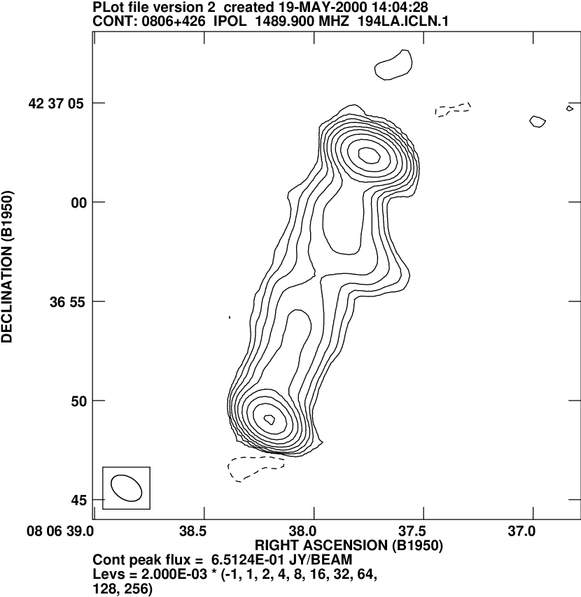
(b)

Figure 4: Radio maps of 3C 194 from archive data in (a) L band and (b) C band.

Radio intensity maps produced from VLA archive data are presented here (Figures 1-6). The 4.872 GHz map of 3C 244.1 was created with a restoring beam identical to the synthesized beam of the 1.411 GHz map of 3C 244.1, and the 4.885 GHz map of 3C 194 was created with a restoring beam identical to the synthesized beam of the 1.465 GHz map of 3C 194. Thus, radio maps at both frequencies for a particular radio galaxy have similar angular resolutions. Radio maps created with three of these archive data sets have appeared in the literature. A 1.411 GHz map of 3C 244.1 appeared in Leahy & Williams (1994), and 4.88 GHz maps of 3C 244.1 and 3C 325 appeared in Fernini, Burns, & Perley (1997).

The computation of $a_{L}$, $B_{L}$, and $v_{L}$ were performed here in the same manner as Wellman, Daly, & Wan (1997a,b). The deconvolved lobe width, $a_{L}$, is measured $10h^{-1}$ kpc from the hot spot toward the host galaxy. The lobe magnetic field strength, $B_{L}$, is computed from the deconvolved surface brightness and bridge width measured $10h^{-1}$ kpc from the hot spot toward the host galaxy. The lobe propagation velocity, $v_{L}$, is computed on the basis of spectral aging along the imaged portions of the bridge, and the magnetic field used in spectral aging is computed using values measured $10h^{-1}$ kpc and $25h^{-1}$ kpc from the hotspot. The errors on each of these quantities are discussed in §5 of WDW97b, §5.2 of WDW97a, and the appendix of this paper.

All parameters presented here are computed with $b=0.25$, which means magnetic fields are computed to be 0.25 times the minimum energy values, and without an $\alpha-z$ correction which refers to a correction related to the observed correlation between spectral index and redshift (see Wellman 1997; Wellman, Daly, Wan 1997a,b; Guerra 1998; Guerra & Daly 1998 for details). It was found by Guerra & Daly (1998) that constraints on cosmological parameters did not depend on these choices, and very similar results are obtained independent of the value of $b$ and of whether an $\alpha-z$ correction is applied.

2.2 Theory

The small dispersion in the average size of 3CR radio galaxies at a given redshift suggests that, at a given redshift, all of the sources have a very similar average size. This size may be estimated by the average size of the full population of powerful extended radio galaxies at that redshift, $<D>$, or by the average size of a given source at that redshift, $D_{*}$. If the total time a source produces powerful jets, with beam power $L_{j}$, that powers the growth and radio emission of the source is $t_{*}$, then the average source size will be $D_{*}=v_{L}~{}t_{*}$, assuming the rate of growth of the source, $v_{L}$, is roughly constant over the source lifetime. The source velocity $v_{L}$, estimated via synchrotron and inverse Compton aging techniques, increases with redshift (Leahy, Muxlow, & Stephens 1989; Liu, Pooley, & Riley 1992; Daly 1994, 1995; WDW97b), and there is no indication that the rate of growth of the sources decreases with redshift. However, the average size of the full population decreases monotonically with redshift for redshifts greater than about 0.5 (see Table 3 in this paper, and Figure 1 in Guerra & Daly 1998).

This means that, for sources of this type, $t_{*}$ must decrease with redshift. For the sources studied here, it was shown by WDW97a that the radio power of a given source is roughly constant over the lifetime of that source, making it very unlikely that the radio power of a given source decreases with time, causing sources at higher redshift to fall below the radio flux limit of the survey when they are smaller.

Thus, since $<D>$ decreases with redshift for $z\;_{\sim}^{>}\;0.5$, and $D_{*}=v_{L}~{}t_{*}$ with $v_{L}$ either increasing with redshift or independent of redshift, the data require that $t_{*}$ decrease with redshift. The rate of growth of the source, $v_{L}$, depends on one parameter that is intrinsic to the AGN, the beam power $L_{j}$, and on two parameters that are extrinsic to the AGN, the ambient gas density $n_{a}$ and the cross sectional area of the radio lobe $\propto a_{L}^{2}$: $v_{L}\propto(L_{j}~{}n_{a}^{-1}~{}a_{L}^{-2})^{(1/3)}$. The total time for which the AGN produces a powerful outflow, $t_{*}$, must depend on properties intrinsic to the black hole, and the only intrinsic parameter that appears in $v_{L}$ is $L_{j}$. Thus, we write $t_{*}\propto L_{j}^{-\beta/3}$, which defines the one model parameter $\beta$. The other intrinsic property of the black hole that might enter is the total energy available to power the outflow, $E_{*}$, but since $E_{*}=L_{j}~{}t_{*}$, any dependence on $E_{*}$ is absorbed into the relation between $t_{*}$ and $L_{j}$.

A power law relation between the total time the AGN produces powerful jets and the beam power of the jets is not unexpected. It means that there is a power law relation between the beam power $L_{j}$ and the total energy available initially $E_{*}$; it is assumed that the beam power is roughly constant over the lifetime of the source, but the value of $L_{j}$ is set by the initial energy available $E_{*}$. This is reminiscent of the power law relation for main sequence stars between luminosity and lifetime, or between total energy available and luminosity for main sequence stars, and of other power law relations that arise so frequently in astrophysics. For example, for a value of $\beta$ of 2, the beam power of the jet is related to the total energy available by the relation $L_{j}\propto E_{*}^{3}$, which is similar to the relation between luminosity and mass for main sequence stars: $L\propto M^{3.5}$. Note, that for main sequence stars, the luminosity is determined by the total energy available initially, and remains roughly constant over the lifetime of the main sequence star. For a value of $\beta$ of 1.5, the relation between beam power and total energy available is $L_{j}\propto E_{*}^{2}$.

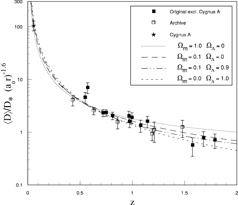
Figure 7: The quantity $(\langle D\rangle/D_{*})(a_{o}r)^{-1.6}$, computed assuming $\beta=1.75$ and $b=0.25$. This measured quantity is independent $\Omega_{m}$ and $\Omega_{\Lambda}$. Open squares denote the six new data points from the VLA archive and Cygnus A is denoted by the star symbol. For different choices of $\Omega_{m}$ and $\Omega_{\Lambda}$, the best-fit redshift evolution of $(a_{o}r)^{-1.6}$ excluding Cygnus A is shown. Note that the fits are not normalized to Cygnus A, but are consistent with Cygnus A.

The excellent fits obtained by comparing $<D>$ with $D_{*}$ assuming that $t_{*}\propto L_{j}^{-\beta/3}$ supports this choice for the parameterization of $t_{*}$. As shown in Figure 7, if the zero-redshift bin containing Cygnus A is excluded from the analysis, and the best fit value of $\beta$ and the constant $C_{ratio}$ (defined below) are determined, we can predict the value of $D_{*}$ for Cygnus A, and it matches the value of $D_{*}$ for Cygnus A to very high accuracy. This is quite extraordinary if we consider the large drop in $<D>$ that occurs from the first redshift bin to the zero-redshift bin, which is mirrored by the large drop in $D_{*}$ of Cygnus A (see Figures 8 and 9).

The theory requires that $D_{*}$ track $<D>$ with redshift, thus it requires

$$<D>/D_{*}=C_{ratio}~{},$$

where $C_{ratio}$ is a constant, independent of redshift. We do NOT require that $<D>/D_{*}=1$, but we require that this ratio is a constant, $C_{ratio}$. Thus, the use of this equation for cosmology is independent of any factor that might be used to normalize the quantity $D_{*}$.

The ratio $<D>/D_{*}$ depends on cosmological parameters and the model parameter $\beta.$ The way that this ratio depends on coordinate distance is given by equation (6) of Guerra & Daly (1998), and the full dependence of $D_{*}$ on observable parameters is given in Appendix A of this paper.

The confidence with which cosmological parameters and the model parameter can be constrained depends on the uncertainty of the ratio $<D>/D_{*}$. This is obtained by combining the uncertainty of $<D>$ and the uncertainty of $D_{*}$ in quadrature. The uncertainty of $<D>$ is given by the dispersion in radio source size at a given redshift. The errors in $<D>$ range from 10 % to 35 % (see Table 3). This dominates the uncertainty of the ratio $<D>/D_{*}$. The uncertainty of $D_{*}$ depends on the uncertainty of each of the quantities used to determine $D_{*}$, and is discussed in detail in Appendix A of this paper.

2.3 Application of the Theory

In terms of quantities that can be estimated from radio observations, $L_{j}\propto v_{L}~{}B_{L}^{2}~{}a_{L}^{2}$ so $D_{*}\propto v_{L}~{}L_{j}^{-\beta/3}$ $\propto v_{L}^{(1-\beta/3)}~{}(B_{L}~{}a_{L})^{-2\beta/3}$ for perfectly symmetric lobes and bridges. The three parameters, $a_{L}$, $B_{L}$, and $v_{L}$ are computed for the bridge on each side of the six radio galaxies obtained from the VLA archive, with the exception of one bridge in 3C 324 which was not imaged along its length sufficiently. The characteristic core-lobe size, $r_{*}$, was computed for each bridge using using the equation described above and in Guerra & Daly (1998), and Daly (1994, 1995):

$$r_{*}\propto\left({1\over B_{L}~{}a_{L}}\right)^{2\beta/3}~{}v_{L}^{1-\beta/3}~{}~{}.$$ (1)

The characteristic (lobe-lobe) size, $D_{*}$, is taken to be the sum of both $r_{*}$ (or in the case of 3C 324, $D_{*}=2r_{*}$), and is normalized so that $D_{*}$ of Cygnus A (3C 405), a very low redshift source in our sample, is equal to the average size of the full population of powerful classical double radio galaxies at very low redshift; this does not impact the determination of the model parameter, $\beta$, or constraints on cosmological parameters, in any way (see §2.2). Constraints on cosmological parameters determined using this method are independent of the normalization of $D_{*}$, as described in §2.2. As discussed in §3.1, the best fit value of the one model parameter $\beta$ is determined simultaneously with the best fit values for the two cosmological parameters that enter, $\Omega_{m}$ and $\Omega_{\Lambda}$, the normalized values of the current values of the mean mass density and the cosmological constant (see Guerra & Daly 1998; Daly, Guerra, & Wan 1998).

Table 2 presents the six new $D_{*}$ values in the last column, assuming the best fit value of $\beta=1.75$ (see §3.1). Source name and redshift are listed in the first two columns. The third column lists the redshift bin corresponding to the assignments in Guerra & Daly (1998) and Table 3 below. The lobe-lobe angular size of the source is listed in the fourth column, the fifth and sixth columns list the core-lobe characteristic sizes, $r_{*}$, and the characteristic source size is listed in column seven.

3 Updated Results

3.1 Constraints on Cosmological Parameters

The subsample of sources with estimates of the characteristic size, $D_{*}$, has been increased from 14 to 20, as discussed above in §2. Only sources with physical sizes, defined as the projected separation between the radio hot spots, greater than $20\,h^{-1}$ kpc can be used to determine a characteristic size. This is because smaller sources are typically not sufficiently resolved so that the radio data are useful, and the radio lobes of smaller sources are interacting with the interstellar medium of the host galaxy rather than the intergalactic/intracluster medium. It was decided that this same criterion should be applied to the larger comparison sample of powerful 3CR radio galaxies. Thus, the sample of radio galaxies used to determine the redshift evolution of the physical size has been reduced from 82 to 70; twelve radio galaxies were cut because the physical separation between their lobes was less than $20\,h^{-1}$ kpc. This has a rather small impact on the actual means and standard deviations of the parent population, as can be seen by comparing Table 3 of this paper with Table 1 of Guerra & Daly (1998). The average lobe-lobe separations as a function of redshift are listed in Table 3 for three example choices of cosmological parameters (matter-dominated, curvature-dominated, and spatially flat with non-zero cosmological constant).

To solve simultaneously for the model parameter $\beta$ and the cosmological parameters $\Omega_{m}$ and $\Omega_{\Lambda}$, the ratio of $D_{*}$ for each source to $\langle D\rangle$, the average lobe-lobe size of the parent population in the corresponding redshift bin, is fit to a constant, independent of redshift: $<D>/D_{*}=C_{ratio}$, where the constant $C_{ratio}$ is allowed to float when the best fit parameters are determined. The value of the constant is a free parameter, so the normalization of $D_{*}$ does not affect the fits in any way.

Figure 7 illustrates the cosmological dependence of $\langle D\rangle/D_{*}$ on the coordinate distance $(a_{o}r)$. As described below, the best fit value of $\beta$ obtained here is $\beta=1.75$; for this value of $\beta$, $\langle D\rangle/D_{*}$ is proportional to $(a_{o}r)^{1.6}$. Thus $(\langle D\rangle/D_{*})(a_{o}r)^{-1.6}$ is independent of cosmological parameters. The data can be compared to several different sets of cosmological parameters on a single figure by plotting $(\langle D\rangle/D_{*})(a_{o}r)^{-1.6}$ for each data point and comparing this with $(a_{o}r)^{-1.6}$ curves obtained for different sets of cosmological parameters, as is shown in Figure 7. Note that, for the fits shown, the lowest redshift bin, which includes Cygnus A, was excluded from the analysis. Even so, the lines all go directly through this point (denoted by a star) indicating the predictive power of this model.

The hypothesis is that, for the correct choice of cosmological parameters, $\langle D\rangle/D_{*}=C_{ratio}$ = constant, so that the values of $(\langle D\rangle/D_{*})(a_{o}r)^{-1.6}$ for all 20 radio galaxies should follow a curve that, at each z, tracks the curve $(a_{o}r)^{-1.6}$ obtained for that particular choice of cosmological parameters. Figure 7, shows $(\langle D\rangle/D_{*})(a_{o}r)^{-1.6}$ for the the six new points and 14 original points as a function of z (the six new points are denoted by open squares). Also drawn on this figure are the best-fit curves of $(a_{o}r)^{-1.6}$ obtained for specified values of cosmological parameters and excluding Cygnus A from the fits. In this figure, all of the curves pass through Cygnus A, though this is not required when we actually solve for best fitting cosmological parameters. Including Cygnus A has a negligible effect on the normalization of these curves and a small effect on cosmological constraints. It is clear that curves obtained for a low density universe describe the data points quite well, and the curve describing a universe with $\Omega_{m}=1$ does not follow the data points.

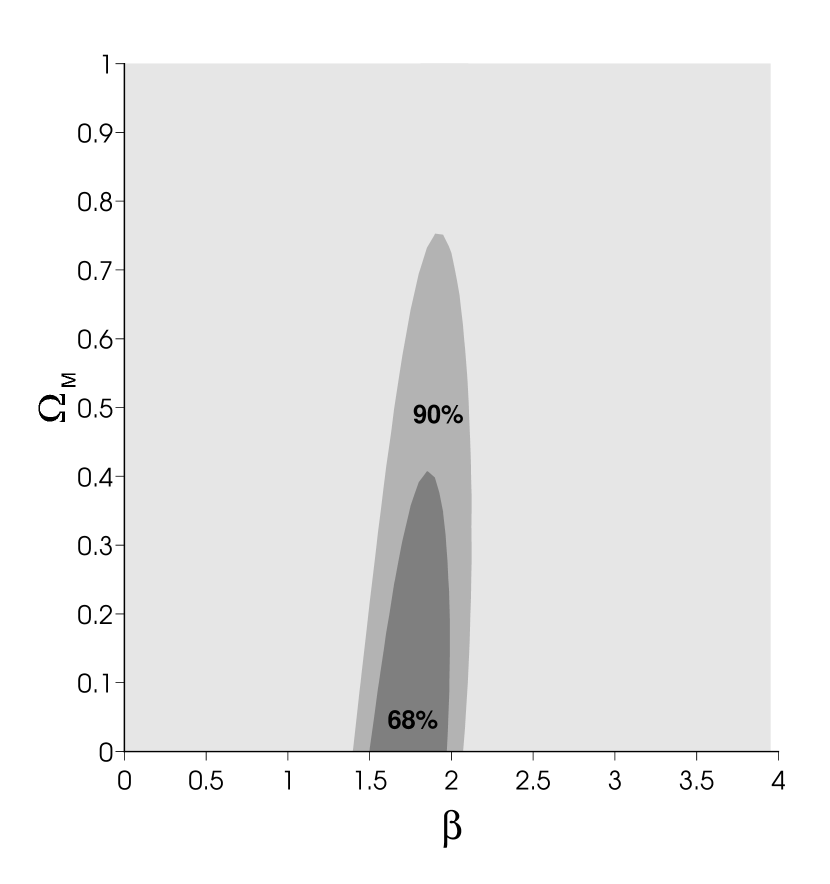
(b)

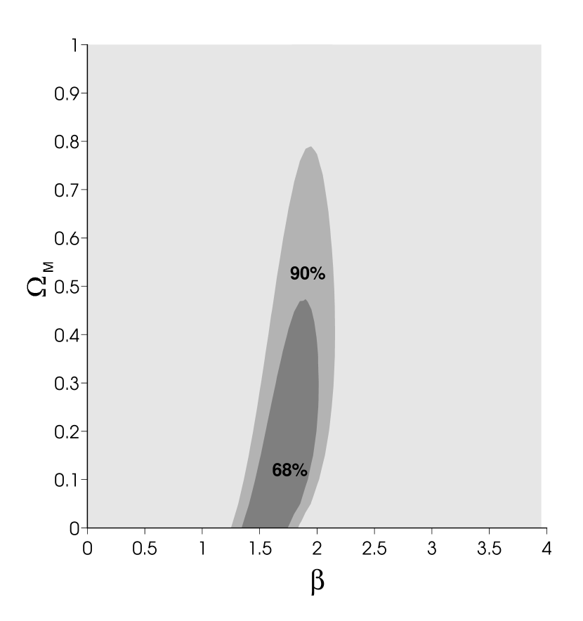
Figure 10: The 68% and 90% confidence intervals for $\beta$ and $\Omega_{m}$, where (a) $\Omega_{\Lambda}$=0 (no cosmological constant)and (b) $\Omega_{\Lambda}=1-\Omega_{m}$ (spatially flat universe).

For all 20 sources, the chi-squared for fitting the ratio to a constant is computed for relevant values of $\beta$, $\Omega_{m}$, and $\Omega_{\Lambda}$. It is found that the best fit value of $\beta$ is $\beta=1.75\pm 0.25$. This result is insensitive to the choice of $\Omega_{m}$ and $\Omega_{\Lambda}$, and there appears to be no significant covariance between $\beta$ and cosmological parameters (see Figures 10a and 10b).

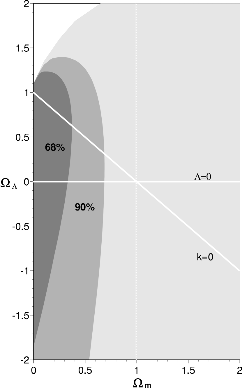
Figure 11: The 68% and 90% confidence intervals for ranges of both $\Omega_{m}$ and $\Omega_{\Lambda}$, independent of $\beta$. (Two-dimensional)

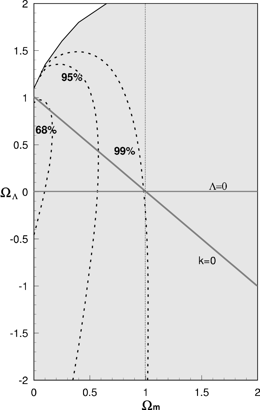
Figure 12: The projections of the 68%, 95%, and 99% confidence intervals onto either axis ($\Omega_{m}$ or $\Omega_{\Lambda}$) indicates the probability associated with the range in that one parameter, independent of all other parameter choices. (One-dimensional)

The confidence contours in the $\Omega_{m}$ - $\Omega_{\Lambda}$ plane are shown in Figures 11 and 12. The probability associated with a given range of $\Omega_{m}$ and $\Omega_{\Lambda}$ independent of $\beta$ is shown in Figure 11 (referred to as two-dimensional confidence intervals). In Figure 12, the projection of a confidence interval onto either axis ($\Omega_{m}$ or $\Omega_{\Lambda}$) indicates the probability associated with a given range of that one parameter, independent of all other parameter choices (referred to as one-dimensional confidence intervals). Both figures illustrate how this method and the data are most consistent with a low density universe; $\Omega_{m}\;{}_{\sim}^{<}\;0.15$ with 68% confidence, $\Omega_{m}\;{}_{\sim}^{<}\;0.5$ with 90% confidence, and $\Omega_{m}\;{}_{\sim}^{<}\;1.0$ with 99% confidence. The constraints on $\Omega_{\Lambda}$ are not as strong, and values of $\Omega_{\Lambda}$ from zero to unity are consistent with the data.

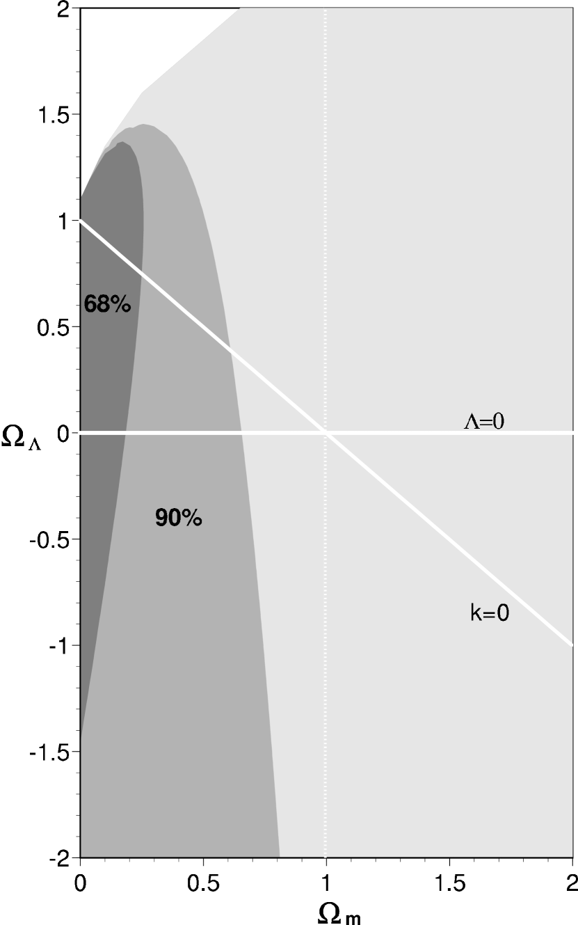
Figure 13: The same as Figure 11, but excluding Cygnus A from the fit.

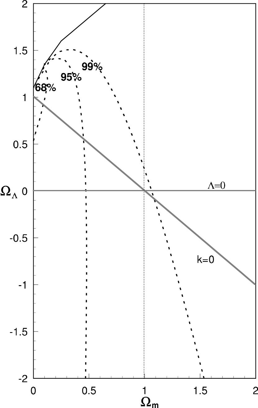
Figure 14: The same as Figure 12, but excluding Cygnus A from the fit.

The best fit value of $\beta=1.75\pm 0.25$ is consistent with the previous estimates of $\beta\simeq 1.5\pm 0.5$ (Daly 1994), and $\beta\simeq 2.1\pm 0.6$ (Guerra & Daly 1996, 1998), but with significantly reduced uncertainties. Similarly, the constraints on cosmological parameters are consistent with previous estimates, (Daly 1994; Guerra & Daly 1996, 1998; Guerra 1997; Daly, Guerra, & Wan 1998) but with smaller error bars. It is apparent in Figures 11 and 12 that these data and method strongly favor a low density universe; a universe where $\Omega_{m}=1$ is ruled out with 99.0 % confidence independent of $\Omega_{\Lambda}$ and $\beta$ . This will be discussed in more detail in §4. To further illustrate the insensitivity of cosmological constraints to including Cygnus A, Figures 13 and 14 show the confidence intervals when Cygnus A is excluded from the fits.

Figures 13 and 14 also illustrate that that data are most consistent with a low density universe. Fits excluding Cygnus A rule out an $\Omega_{m}=1$ universe at 97.5% confidence. These results are quite similar to those obtained when Cygnus A is included. This further illustrates that the method does not rely upon a low-redshift normalization.

3.2 Ambient Gas Densities and Beam Powers

Daly (1994, 1995, 2000), following the work of Perley & Taylor (1991), Carilli et. al (1991), and Rawlings & Saunders (1991), showed that the radio properties of a powerful extended radio source could be used to estimate the beam power, $L_{j}$, and density of the gas in the vicinity of the source, $n_{a}$. The method is described in detail by Wellman (1997), Wellman, Daly, & Wan (1997a), Wan (1998), Wan, Daly, & Guerra (1998), and Daly (2000). Values for the ambient gas density and beam power for the 14 sources in the original sample are described in these papers. The basic equations are:

$$L_{j}\propto a_{L}^{2}~{}P_{L}~{}v_{L}~{}~{},$$ (2)

and

$$n_{a}\propto{P_{L}\over v_{L}^{2}}~{}~{};$$ (3)

where $P_{L}$ is the lobe pressure (see equation A2), and the normalizations are given in the references listed above. The values obtained for the six new radio galaxies in our sample are listed in Table 4. Also listed in Table 4 are all the input parameters used to compute $L_{j}$, $n_{a}$, and $D_{*}$.

4 Discussion

A parent population of 70 powerful extended classical double radio galaxies with redshifts between zero and two was used to define the evolution of the mean or characteristic size of these sources as a function of redshift; these sources are all Type 1 FRII sources (Leahy & Williams 1984), also referred to as FRIIb sources (Daly 2000). An independent estimate of the mean or characteristic size of a given source was possible for a subset of 20 of these radio galaxies for which extensive multiple frequency radio data was available. Requiring that the two measures of the mean source size have the same redshift behavior allows a simultaneous determination of three parameters: the one model parameter $\beta$, and the two cosmological parameters $\Omega_{m}$ and $\Omega_{\Lambda}$ (assuming that the only significant cosmological parameters today are the mean mass density, a cosmological constant, and space curvature).

The method was applied to this data set, and interesting new constraints are presented. It is found that the model parameter is very tightly constrained to be $\beta=1.75\pm 0.25$ (see Figure 10), consistent with previous estimates, and that this model parameter is independent of cosmological parameters. For a value of $\beta=1.75$, the characteristic source size is $D_{*}\propto(B_{L}a_{L})^{-7/6}~{}{v_{L}}^{5/12}$, which indicates that it is necessary to have multiple-frequency radio data in order to estimate $D_{*}$, owing to its $v_{L}$ dependence.

The data strongly favor a low density universe; a universe with $\Omega_{m}=1$ is ruled out with 99% confidence, independent of the value of $\Omega_{\Lambda}$ or $\beta$. Either space curvature or a cosmological constant, or both, are allowed. The main conclusion is that $\Omega_{m}$ is low, but, at this point, the method and data do not allow a discrimination between whether space curvature or a cosmological constant is important at the present epoch.

It is interesting to note that the lowest reduced chi-squared obtained is 0.96 for $\Omega_{m}\simeq-0.25$ and $\Omega_{\Lambda}\simeq 0$. This value is slightly greater and closer to unity than the minimum reduced chi-squared obtained by Guerra & Daly (1998), which indicates that this sample of 20 sources has a reasonable distribution around any model predictions. This convergence to unity with increasing sample size suggests that this method and its statistics are reliable.

The best fit for cosmological parameters in the physically relevant half-plane of $\Omega_{m}\;{}_{\sim}^{>}\;0$ is $\Omega_{m}=0$ and $\Omega_{\Lambda}=0.45$ with a reduced chi-squared of 0.98 (also close to unity). However, Figures 11 and 12 clearly show that our results are still consistent with $\Omega_{\Lambda}=0$.

The radio data also allow a determination of the density of the ambient gas in the vicinity of each radio source, and the beam power of each source; the values of these quantities are presented. The sources lie in high-density gaseous environments like those found in low-redshift clusters of galaxies. Typical beam powers for the sources are $\sim 10^{45}\hbox{ erg s}^{-1}$.

Appendix A Error Analysis

Errors on $D_{*}$ and errors on $<D>$ both contribute to the confidence contours relevant for the cosmological parameters determined here. The errors on $<D>$ are purely statistical, and arise from the dispersion in source size of the parent population, and at the present time dominate the total uncertainty of the quantity $<D>/D_{*}$. The errors on $D_{*}$ depend on the uncertainties of quantities used to determine $D_{*}$; the way that the error on $D_{*}$ is computed is presented here.

The quantity

$$r_{*}=v_{L}~{}t_{*}\propto v_{L}~{}L_{j}^{-\beta/3}\propto v_{L}\left(P_{L}~{}v_{L}~{}a_{L}^{2}\right)^{-\beta/3}\propto v_{L}^{1-\beta/3}~{}a_{L}^{-2\beta/3}~{}P_{L}^{-\beta/3}.$$ (A1)

The lobe pressure

$$P_{L}\propto\left(\frac{4}{3}~{}b^{-1.5}+b^{2}\right)~{}B_{min}^{2},$$ (A2)

where $B_{min}$ is the minimum energy magnetic field, $B_{min}\propto S_{\nu}^{2/7}~{}a_{L}^{-2/7}$, and is determined using parameters obtained 10 $h^{-1}$ kpc behind the hotspot: the radio surface brightness at this location is $S_{\nu,10}$ and the lobe half-width at this location is $a_{L,10}$. The radio surface brightness and lobe half-width 25 $h^{-1}$ kpc behind the hotspot are denoted $S_{\nu,25}$ and $a_{L,25}$ respectively. The lobe propagation velocity $v_{L}$ is estimated using a standard synchrotron and inverse Compton aging model in which the time, $t$, required for the source to grow a size $\Delta x$, is used to estimate the lobe propagating velocity $v_{L}=\Delta x/t$. The time

$$t\propto\frac{B_{av}^{1/2}}{\nu_{T}^{1/2}\left(B_{av}^{2}+B_{MB}^{2}\right)}$$ (A3)

(see, for example, Wan & Daly 1998, §3) where $\nu_{T}$ is the break frequency, $B_{av}$ is the average magnetic field in the radio bridge, taken to be $B_{av}=\sqrt{B_{10}B_{25}}$ (WDW97b), $B_{10}$ is the magnetic field strength 10 $h^{-1}$ kpc behind the hotspot, $B_{25}$ is the magnetic field strength 25 $h^{-1}$ kpc behind the hotspot, and $B_{MB}$ is the term that describes inverse Compton cooling of relativistic electrons by scattering with microwave background photons, and is obtained by equating the energy density of the microwave background at a given redshift with $B_{MB}^{2}/(8\pi)$.

In terms of these parameters,

$$r_{*} \propto \left(\frac{4}{3}~{}b^{-1.5}+b^{2}\right)^{-\beta/3}~{}B_{10}^{-2\beta/3}~{}a_{L}^{-2\beta/3}~{}\Delta x^{(1-\beta/3)}~{}\nu_{T}^{\frac{1}{2}(1-\beta/3)}$$

$$\times\left(B_{av}^{2}+B_{MB}^{2}\right)^{1-\beta/3}~{}B_{10}^{-\frac{1}{4}(1-\beta/3)}~{}B_{25}^{-\frac{1}{4}(1-\beta/3)}.$$

Given that the magnetic field strength is parameterized by $B=b~{}B_{min}$ at any given location, we obtain the following expression for $r_{*}$, which is relevant for a determination of the error:

$$r_{*} \propto \left(\frac{4}{3}b^{-1.5}+b^{2}\right)^{-\beta/3}b^{-\frac{1}{2}(1+\beta)}~{}\Delta x^{(1-\beta/3)}~{}{\nu_{T}}^{\frac{1}{2}(1-\beta/3)}~{}{B_{25}}^{\frac{1}{4}(\beta/3-1)}~{}{a_{L,10}}^{-\frac{1}{2}(\beta-1/7)}~{}$$

$$\times{S_{\nu,10}}^{-(\beta/6+1/14)}~{}\left(b^{2}~{}{S_{\nu,10}}^{2/7}~{}{S_{\nu,25}}^{2/7}~{}{a_{L,10}}^{-2/7}~{}{a_{L,25}}^{-2/7}+{B_{MB}}^{2}\right)^{(1-\beta/3)}.$$

The total error on $\delta r_{*}/r_{*}$ is found by taking the partial derivative of $r_{*}$ with respect to a given variable, for each variable, adding these terms in quadrature, and taking the square-root. We obtain

$$\left(\frac{\delta r_{*}}{r_{*}}\right)_{\nu_{T}}=\frac{1}{2}~{}(1-\beta/3)\left(\frac{\delta\nu_{T}}{\nu_{T}}\right)$$ (A6)

$$\left(\frac{\delta r_{*}}{r_{*}}\right)_{\Delta x}=(1-\beta/3)\left(\frac{\delta\Delta x}{\Delta x}\right)$$ (A7)

$$\left(\frac{\delta r_{*}}{r_{*}}\right)_{B_{25}}=\left[-\frac{1}{4}(1-\beta/3)+(1-\beta/3)\left(\frac{B_{10}B_{25}}{B_{10}B_{25}+{B_{MB}}^{2}}\right)\right]\left(\frac{\delta B_{25}}{B_{25}}\right)$$ (A8)

$$\left(\frac{\delta r_{*}}{r_{*}}\right)_{a_{L,10}}=\left[\frac{1}{2}(1/7-\beta)-\frac{2}{7}(1-\beta/3)\left(\frac{B_{10}B_{25}}{B_{10}B_{25}+{B_{MB}}^{2}}\right)\right]\left(\frac{\delta a_{L,10}}{a_{L,10}}\right)$$ (A9)

$$\left(\frac{\delta r_{*}}{r_{*}}\right)_{S_{\nu,10}}=\left[-(\beta/6+1/14)+\frac{2}{7}(1-\beta/3)\left(\frac{B_{10}B_{25}}{B_{10}B_{25}+{B_{MB}}^{2}}\right)\right]\left(\frac{\delta S_{\nu,10}}{S_{\nu,10}}\right)$$ (A10)

$$\left(\frac{\delta r_{*}}{r_{*}}\right)_{b}=\left[\frac{2\beta}{3}\left(\frac{1-b^{3.5}}{4/3+b^{3.5}}\right)-\frac{1}{2}(1+\beta)+(1-\beta/3)\left(\frac{2B_{10}B_{25}}{B_{10}B_{25}+{B_{MB}}^{2}}\right)\right]\left(\frac{\delta b}{b}\right)$$ (A11)

The final uncertainty of $r_{*}$ divided by $r_{*}$, $\delta r_{*}/r_{*}$ is obtained by adding each of the terms listed above in quadrature, and taking the square root. As mentioned above, this is typically much less than the uncertainty of $<D>$, so the confidence level with which cosmological parameters are determined is primarily controlled by the uncertainty in $<D>$ (see Table 3).

The uncertainties on each of the quantities listed above are described in section 5 of WDW97b, and section 5.2 of WDW97a. The uncertainty in $\nu_{T}$ is typically (10 to 20) %. The uncertainty on $\Delta x$ is typically (6 to 20) %. The uncertainty on $B_{25}$ is typically 6 %. The uncertainty on $a_{L,10}$ is typically (6 to 20)%; this term (et. A9) is generally the largest contribution to the error in $r_{*}$. The uncertainty on $S_{\nu,10}$ is typically 20 %, and the uncertainty on b is about 15 % for b = 0.25, and is about 10 % for b = 1 (see Wellman, Daly,& Wan 1997b, section 7.4).

For a given value of $\beta$, equations A6 through A11 may be written as a number times the fractional error on the relevant quantity. Some of the equations involve the fraction $f=\left(\frac{B_{10}B_{25}}{B_{10}B_{25}+{B_{MB}}^{2}}\right)$, which is always less than or equal to one. To get a sense of which terms contribute to the total error in $r_{*}$, equations A6 through A11 are rewritten assuming a value of $\beta$ of 1.75.

$$\left(\frac{\delta r_{*}}{r_{*}}\right)_{\nu_{T}}\simeq 0.21\left(\frac{\delta\nu_{T}}{\nu_{T}}\right)$$ (A12)

$$\left(\frac{\delta r_{*}}{r_{*}}\right)_{\Delta x}\simeq 0.42\left(\frac{\delta\Delta x}{\Delta x}\right)$$ (A13)

$$\left(\frac{\delta r_{*}}{r_{*}}\right)_{B_{25}}=(-0.10+0.42f)\left(\frac{\delta B_{25}}{B_{25}}\right)$$ (A14)

$$\left(\frac{\delta r_{*}}{r_{*}}\right)_{a_{L,10}}=(-0.80-0.12f)\left(\frac{\delta a_{L,10}}{a_{L,10}}\right)$$ (A15)

$$\left(\frac{\delta r_{*}}{r_{*}}\right)_{S_{\nu,10}}=(-0.36+0.12f)\left(\frac{\delta S_{\nu,10}}{S_{\nu,10}}\right)$$ (A16)

$$\left(\frac{\delta r_{*}}{r_{*}}\right)_{b=1}=(-1.375+0.83f)\left(\frac{\delta b}{b}\right)$$ (A17)

$$\left(\frac{\delta r_{*}}{r_{*}}\right)_{b=0.25}=(-0.51+0.83f)\left(\frac{\delta b}{b}\right)$$ (A18)

The largest contribution to the uncertainty in $r_{*}$ is usually due to the uncertainty in the bridge width $a_{L,10}$.

Table 1: VLA Archive Data Sets

			Listed	Frequency	Array
Source	Band	Program ID	Observer	(GHz)	Config.	Date
3C 244.1	L	POOL	Pooley, G.	1.411	B	09/17/82
	C	AF213	Fernini, I.	4.872	B	12/23/91
3C 337	L	AR123	Rudnick, L.	1.452	A	02/21/85
	C	AR123	Rudnick, L.	4.885	B	06/01/85
3C 325	L	AV153	van Breugel, W.	1.465	A	12/05/88
	C	AF213	Fernini, I.	4.885	B	12/23/91
3C 194	L	AV164	van Breugel, W.	1.465	A	05/11/90
	C	AV164	van Breugel, W.	4.885	A	05/11/90
3C 324	L	AR123	Rudnick, L.	1.452	A	02/21/85
	C	AR123	Rudnick, L.	4.885	B	06/01/85
3C 437	L	AV164	van Breugel, W.	1.465	A	05/11/90
	C	AV164	van Breugel, W.	4.885	B	04/21/89

Table 2: Radio Galaxies with $D_{\star}$ Presented Here

			$\theta$	$r_{\star}$		$D_{\star}$
Source	$z$	Bin	(arcsec)	($h^{-1}$ kpc)	($h^{-1}$ kpc)	($h^{-1}$ kpc)
3C 244.1	0.43	2	50.8	$151\pm 16$	$135\pm 16$	$286\pm 22$
3C 337	0.63	3	43.5	$150\pm 24$	$65\pm 7$	$214\pm 25$
3C 325	0.86	3	15.8	$164\pm 52$	$66\pm 14$	$230\pm 54$
3C 194	1.19	4	14.2	$105\pm 22$	$92\pm 15$	$197\pm 27$
3C 324	1.21	5	10.2	$75\pm 18$	$\cdots$	$149\pm 35$
3C 437	1.48	5	36.7	$55\pm 6$	$48\pm 5$	$103\pm 8$

Table 3: The Average Lobe-Lobe Sizes for Powerful 3CR Radio Galaxies.

				$\langle D\rangle$ ($h^{-1}$ kpc)
Bin	$z$ Range	Sources		$\Omega_{o}=1.0$, $\Omega_{\Lambda}=0.0$	$\Omega_{o}=0.1$, $\Omega_{\Lambda}=0.0$	$\Omega_{o}=0.1$, $\Omega_{\Lambda}=0.9$
1	0.0-0.3	3		66$\pm$14	68$\pm$14	72$\pm$13
2	0.3-0.6	13		202$\pm$45	224$\pm$50	259$\pm$57
3	0.6-0.9	23		148$\pm$17	174$\pm$20	209$\pm$24
4	0.9-1.2	16		107$\pm$24	133$\pm$29	165$\pm$36
5	1.2-1.6	9		91$\pm$32	122$\pm$43	152$\pm$53
6	1.6-2.0	6		66$\pm$19	92$\pm$26	114$\pm$33

Table 4: Summary of New Source Properties

Source	$z$	$r$	$a_{L}$	$B_{10}$	$B_{25}$	$v_{L}$	$n_{a}$	$\log L_{j}$
244.1	0.43	101	$5.5\pm 0.3$	$3.5\pm 0.2$	$2.5\pm 0.2$	$1.1\pm 0.2$	$1.0\pm 0.4$	$44.35\pm 0.10$
		91.6	$4.7\pm 0.4$	$5.3\pm 0.3$	$3.2\pm 0.2$	$1.7\pm 0.3$	$1.0\pm 0.4$	$44.75\pm 0.11$
337	0.63	125	$6.2\pm 0.5$	$3.5\pm 0.2$	$2.3\pm 0.1$	$1.5\pm 0.5$	$0.6\pm 0.4$	$44.57\pm 0.15$
		69.8	$10.5\pm 0.4$	$3.8\pm 0.2$	$2.8\pm 0.2$	$1.1\pm 0.2$	$1.2\pm 0.4$	$44.99\pm 0.10$
325	0.86	49.0	$3.3\pm 1.1$	$6.8\pm 0.9$	$4.0\pm 0.3$	$2.0\pm 0.5$	$1.2\pm 0.6$	$44.73\pm 0.23$
		34.7	$4.4\pm 0.8$	$12.7\pm 1.0$	$4.6\pm 0.3$	$3.0\pm 0.8$	$1.9\pm 1.0$	$45.70\pm 0.17$
194	1.19	31.6	$4.5\pm 1.0$	$7.1\pm 0.6$	$5.0\pm 0.3$	$1.8\pm 0.3$	$1.6\pm 0.6$	$45.00\pm 0.16$
		50.0	$5.6\pm 0.8$	$6.7\pm 0.5$	$5.6\pm 0.4$	$2.0\pm 0.3$	$1.2\pm 0.4$	$45.16\pm 0.13$
324	1.21	22.1	$4.5\pm 0.9$	$10.3\pm 0.9$	$\cdots$	$2.1\pm 0.7$	$2.4\pm 1.5$	$45.38\pm 0.19$
437	1.48	106	$11.4\pm 0.8$	$6.9\pm 0.4$	$4.2\pm 0.2$	$4.6\pm 0.8$	$0.2\pm 0.1$	$46.18\pm 0.10$
		101	$10.5\pm 0.8$	$9.4\pm 0.6$	$6.7\pm 0.4$	$6.0\pm 1.0$	$0.2\pm 0.1$	$46.49\pm 0.10$

(a)

(b)

Figure 1: Radio maps of 3C 244.1 from archive data in (a) L band and (b) C band.

(a)

(b)

Figure 2: Radio maps of 3C 337 from archive data in (a) L band and (b) C band.

(a)

(b)

Figure 3: Radio maps of 3C 325 from archive data in (a) L band and (b) C band.

(a)

(a)

(b)

Figure 5: Radio maps of 3C 324 from archive data in (a) L band and (b) C band.

(a)

(b)

Figure 6: Radio maps of 3C 437 from archive data in (a) L band and (b) C band.

Figure 8: The average lobe-lobe size $\langle D\rangle$ of powerful extended 3CR radio galaxies computed assuming $\Omega_{m}=0.1$ and $\Omega_{\Lambda}=0$.

Figure 9: The quantity $D_{*}$ computed assuming $\beta=1.75$, $b=0.25$, $\Omega_{m}=0.1$, and $\Omega_{\Lambda}=0$. Open squares denote the six new data points from the VLA archive and Cygnus A is denoted by the star symbol.

(a)

References

- Bennett (1962) Bennett, A. S. 1962, MmRAS, 68, 163
- Carilli etal (1991) Carilli, C. L., Perley, R. A., Dreher, J. H. & Leahy, J. P. 1991, ApJ, 383, 554
- Daly (1994) Daly, R. A. 1994, ApJ, 426, 38
- Daly (1995) Daly, R. A. 1995, ApJ, 454, 580
- Daly (2000) Daly, R. A. 2000, in Lifecylces of Radio Galaxies, in press
- Daly (1996) Daly, R. A. 1996, in IAU 175: Extragalactic Radio Sources, ed. C. Fanti (Dordrecht: Kluwer), 319
- Daly, Guerra, & Wan (1998) Daly, R. A., Guerra, E. J., & Wan, L. 1998, in Fundamental Parameters in Cosmology, ed. J. Trân Thanh Vân & Y. Giraud-Heraud, (Paris: Editions Frontieres), in press
- Fanaroff & Riley (1974) Fanaroff, B. L. & Riley, J. M. 1974, MNRAS, 167, 31
- (9) Fernini, I., Burns, J. O., & Perley, R. A. 1997, AJ, 114, 2292
- Guerra (1997) Guerra, E. J. 1997, Ph.D. thesis, Princeton University
- Guerra & Daly (1996) Guerra, E. J. & Daly, R. A. 1996, in Cygnus A: Study of a Radio Galaxy, ed. C. Carilli & D. Harris (Cambridge: Cambridge University Press), 252
- Guerra & Daly (1998) Guerra, E. J. & Daly, R.A. 1998, ApJ, 493, 536.
- Leahy, Muxlow, & Stephens (1989) Leahy, J. P., Muxlow, T. W., & Stephens, P. W. 1989, MNRAS, 239, 401
- Leahy & Williams (1984) Leahy, J. P & Williams, A. G. 1989, MNRAS, 210, 929
- Liu, Pooley, & Riley (1992) Liu, R., Pooley, G., & Riley, J. M. 1992, MNRAS, 257, 545
- Myers & Spangler (1985) Myers, S. T. & Spangler, S. R. 1985, ApJ, 291, 52
- Perley & Taylor (1991) Perley, R. A., & Taylor, G. B. 1991, AJ, 101, 1623
- Rawlings & Saunders (1991) Rawlings, S., & Saunders, R. 1991, Nature, 349, 138
- Wan (1998) Wan, L. 1998, Ph.D. thesis, Princeton University
- (20) Wan, L. & Daly, R. A. 1998a, ApJS, 115, 141
- (21) Wan, L. & Daly, R. A. 1998b, ApJ, 499, 614
- Wan, Daly, & Guerra (1998) Wan, L., Daly, R. A., & Guerra, E. J. 2000, ApJ, in press
- Wan, Daly, & Wellman (1996) Wan, L., Daly, R. A., & Wellman, G. F. 1996, in Energy Transport in Radio Galaxies and Quasars, ed. P. Hardee, A. Bridle, & J. Zensus, (San Francisco: ASP Conf. Proc.), 305
- Wellman (1997) Wellman, G. F. 1997, Ph.D. thesis, Princeton University
- (25) Wellman, G. F & Daly, R. A. 1996a, in Cygnus A: Study of a Radio Galaxy, ed. C. Carilli & D. Harris (Cambridge: Cambridge University Press), 215
- (26) Wellman, G. F & Daly, R. A. 1996b, in Cygnus A: Study of a Radio Galaxy, ed. C. Carilli & D. Harris (Cambridge: Cambridge University Press), 246
- (27) Wellman, G. F., Daly, R. A., & Wan, L. 1997a, ApJ, 480, 79 (WDW97a)
- (28) Wellman, G. F., Daly, R. A., & Wan, L. 1997b, ApJ, 480, 96 (WDW97b)