The Size and Shape of Voids in Three-Dimensional Galaxy Surveys

Abstract

The sizes and shapes of voids in a galaxy survey depend not only on the physics of structure formation, but also on the sampling density of the survey and on the algorithm used to define voids. Using an N-body simulation with a $\tau$CDM power spectrum, we study of the properties of voids in samples with different number densities of galaxies, both in redshift space and in real space. When voids are defined as totally empty regions of space, their characteristic volume is strongly dependent on sampling density; when they are defined as regions whose density is 0.2 times the mean galaxy density, the dependence is less strong. We compare two void-finding algorithms, one in which voids are nonoverlapping spheres, and one, based on the algorithm of Aikio & Mähönen, which does not predefine the shape of a void. Regardless of the algorithm chosen, the characteristic void size is larger in redshift space than in real space, and is larger for low sampling densities than for high sampling densities. We define an elongation statistic $Q$ which measures the tendency of voids to be stretched or squashed along the line of sight. Using this statistic, we find that at sufficiently high sampling densities (comparable to the number density of $L>L_{*}$ galaxies), large voids tend to be slightly elongated along the line of sight in redshift space.

1 Introduction

When the positions of galaxies are mapped in redshift space, the nature of the large-scale structure seen in the maps is “frothy” or “bubbly”. Voids – regions in which there are few or no galaxies – fill much of the map. The galaxies exist mainly in thin filaments or sheets that lie between the voids. Comparison of the observed pattern of voids with that predicted by a given model of structure formation is potentially a very powerful test for acceptance or rejection of that model. Unfortunately, the differences between models are often subtle. Many models for structure formation predict a bubbly galaxy distribution. In the gravitational instability scenario, regions that are originally underdense expand faster than the Hubble flow (Fillmore & Goldreich, 1984; Bertschinger, 1985). As underdense regions expand, they become more nearly spherical (Fujimoto, 1983; Icke, 1984; Blaes, Goldreich, & Villumsen, 1990). Whether voids in the actual universe are viewed as isolated spherical structures or as a space-filling foam depends on the density level at which voids are defined (Gott, Melott, & Dickinson, 1986). Van de Weygaert & van Kampen (1993) did extensive studies of voids in constrained Gaussian fields, finding that voids become nearly spherical in their very underdense inner regions, while their boundary regions remain more irregular.

If structure grows via gravitational instability, then the size and shape of voids depends on the initial power spectrum $P(k)$ for the density fluctuations and on the density parameter $\Omega$. In an open universe, void evolution stops when $\Omega\sim 0.5$; thereafter, the void network simply expands along with the Hubble flow (Regös & Geller, 1991). At a given epoch, the mean void radius is proportional to the nonlinearity scale $k_{\rm nl}$ (Kauffmann & Melott, 1992). The full distribution of void sizes, however, depends on the shape of the spectrum $P(k)$ (Melott, 1987; Ryden & Melott, 1996).

If we know with absolute accuracy the position of galaxies in real space, we could use the spectrum of void sizes to place constraints on the initial power spectrum $P(k)$. However, measuring the distances to galaxies is difficult; it is much easier to measure their redshifts. Consequently, practical studies of the properties of voids must take place in redshift space rather than real space. If all galaxies smoothly followed the Hubble flow, with no peculiar velocities, and if the Hubble constant $H_{0}$ were truly constant with time, then the mapping between real space and redshift space would be linear. Generally, though, the Hubble constant changes with time, and structure that is isotropic in real space becomes distorted along the line of sight in redshift space, with the amount of distortion increasing with redshift $z$ (Alcock & Paczyński, 1979). Potentially, distortions in the shapes of voids in redshift space can provide an estimate of the deceleration parameter $q_{0}$ (Ryden, 1995). However, the distortions that result from cosmological effects become large only when $z\sim 1$. In the nearby universe, where $z<1$, the dominant contribution to distortions from redshift space comes from the peculiar velocity of galaxies. Ryden & Melott (1996) demonstrated, for instance, that in two-dimensional simulations with $P(k)\propto k^{n}$, the characteristic void size is larger in redshift space than in real space. Redshift space distortions can also, in principle, be harnessed to measure $\Omega_{m}$, the density in nonrelativistic matter (Melott et al., 1998). One goal of this paper is to extend the analysis of Ryden & Melott (1996) to three-dimensional simulations with more realistic CDM power spectra.

Analyzing the properties of voids first requires a definition of what a void is. Some of the statistics used to describe voids define a void as a region totally devoid of galaxies. The void probability function (VPF) is one such statistic; the VPF $P_{0}(V)$ is the probability that a randomly positioned sphere of volume $V$ contains no galaxies (White, 1979). However, the random dilution of a point process (selecting only a fraction of all the galaxies in the universe, for instance), although it leaves the correlation function unchanged, strongly affects VPF (Sheth, 1996). Thus, from a practical viewpoint, it makes more sense to define a void which is underdense with respect to the average number density of galaxies. Little & Weinberg (1994), for instance, use the underdense probability function (UPF). The UPF $P_{f}(V)$ can be defined as the probability that a randomly positioned sphere of volume $V$ contains a number density of galaxies less than or equal to $f$ times the average number density of galaxies in the entire survey. We will follow Little & Weinberg (1994) in setting a void threshold of $f=0.2$, matching the density contrast of the largest voids in the CfA redshift survey (Vogeley, Geller, & Huchra, 1991; Vogeley et al., 1994). One advantage of the UPF over the VPF is that it is relatively insensitive to the sparseness with which the galaxies are sampled. In this paper, we will explicitly compare the UPF and VPF for different galaxy sampling densities.

In addition to statistical measurements such as the VPF and UPF, algorithms exist that identify individual voids within a sample (Kauffmann & Fairall, 1991; Kauffmann & Melott, 1992; Ryden, 1995; Ryden & Melott, 1996; El-Ad & Piran, 1997; Aikio & Mähönen, 1998). In addition to providing a spectrum of void sizes, these void-detection algorithms also enable us to specify the location and shape of individual voids. In this paper, we first use an algorithm (an extension of the two-dimensional algorithm of Ryden [1995]) which defines voids as non-overlapping underdense spheres. Although this algorithm is conceptually simple, it has the disadvantage of forcing voids to be spherical. Thus, we also employ a more sophisticated algorithm, based on that of Aikio & Mähönen (1998; AM), which does not constrain voids to be any particular shape. The original AM algorithm defines voids as empty regions; our modification of the original defines voids as underdense regions. For the voids found by the modified AM algorithm, we introduce an elongation statistic $Q$ which measures whether the voids are stretched or squashed along the line of sight from the origin. Just as with the UPF and VPF, we also apply the void-detection algorithms to different sampling densities of the same survey. Our studies of void properties in numerical simulations will permit a more effective interpretation and understanding of voids in future three-dimensional redshift surveys.

In section 2, we describe the N-body simulation analyzed in this paper. In section 3, we examine the statistical properties of voids, as given by the VPF and UPF. In section 4, we apply void-detection algorithms to the simulations. Finally, in section 5, we analyze the effects of peculiar velocities and galaxy sampling density on void properties, and discuss implications for future work.

2 The Numerical Simulation

The simulation used for testing in this paper was done using a particle-mesh (PM) N-body simulation. The PM method is quite fast, and with a mean particle density of one per simulation cell, represents the maximum resolution that can be achieved without introducing two-body scattering that decouples the result from its initial conditions on small scales (Kuhlman, Melott, & Shandarin, 1996; Splinter et al., 1998). The simulation used here had 256³ particles on a 256³ mesh. Initial conditions were generated by Fast Fourier Transform with random phase perturbations. Since behavior at high density peaks is not of interest to us in our study of voids, the simulations were begun with an RMS density of 0.25 at the resolution limit. The simulations were evolved until the RMS overdensity inside a randomly located sphere of radius $8h^{-1}{\rm\,Mpc}$ was $\sigma_{8}=1.05$.

A matter-dominated Friedman-Robertson-Walker background density was assumed, with the cosmological constant $\Lambda$ set equal to zero. Since nonlinear modes are filtered out, and the dynamical effect of nonzero $\Omega_{\Lambda}$ is well-understood in perturbation theory (Lahav et al., 1991), we did not use nonzero values of $\Lambda$. The value of $\Omega_{m}$, the dimensionless matter density, was taken to be $\Omega_{m}=1$. The box size was take to be 1536 Mpc and the Hubble constant $h=H_{0}/100{\rm\,km}{\rm\,s}^{-1}{\rm\,Mpc}^{-1}=0.75$. Thus, the box size in redshift space corresponds to $1.152\times 10^{5}{\rm\,km}{\rm\,s}^{-1}=0.384c$. Formally, in the simulation $h$ only sets an overall timescale; since both the expansion rate and the particle velocities scale with $h$, the redshift space appearance does not change with $h$, only its overall scale.

The initial power spectrum we assume is a cold dark matter (CDM) spectrum, in which the parameter $\Gamma$ determines the shape of the spectrum. Smaller values of $\Gamma$ are favored today, because they push the turnover in the slope of the power spectrum to large scales, in better agreement with observations. To test our void-finding algorithms, we use $\Gamma=0.25$. Normally, $\Gamma$ is taken to be $\Omega_{0}h$, as the turnover scale is set by the horizon at the end of the radiation-dominated era. However, we break this assumed coupling and take $\Gamma$ as a free parameter descriptive of the spectral shape. Thus, our model corresponds to what is sometimes called $\tau$CDM.

The number density of mass points in the simulation, $n=4.63\times 10^{-3}{\rm\,Mpc}^{-3}$, corresponds to the number density of galaxies with $L>0.42L_{*}$, assuming that the luminosity function of galaxies is a Schechter function with slope $\alpha=-1.07$ and normalization $\Phi_{*}=6.75\times 10^{-4}{\rm\,Mpc}^{-3}$ (Efstathiou, Ellis, & Peterson, 1988). One purpose of this paper is to investigate the dependence of void properties on the sampling density of a galaxy survey. Thus, from the initial numerical simulation, we have created three different samples, corresponding to volume-limited surveys with different luminosity cutoffs. To create our densest sample, we randomly selected a fraction $X=0.82$ of the initial mass points, in order to match the number density of galaxies with $L>L_{*}/2$. For the next densest sample, we selected a fraction $X=0.31$ of the mass points, to match the number density of galaxies with $L>L_{*}$. Finally, for our least dense sample, we selected a fraction $X=0.067$ of the mass points, to match the density of galaxies with $L>2L_{*}$. Note that by randomly selecting galaxies in this way, we are assuming that galaxies are unbiased with respect to the mass distribution, and that luminosity segregation does not exist. We wish to study only the effects of different sampling densities, and not the more subtle effects of bias.

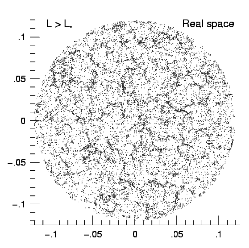
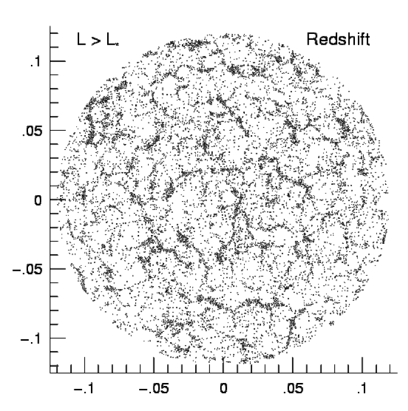
Figure 1: (a) A slice of thickness $12h^{-1}{\rm\,Mpc}$ through the N-body simulation analyzed in this paper. The number density of mass points is chosen to be comparable to the observed number density of galaxies with $L>L_{*}$. (b) A slice of the same thickness through the same sample, but with peculiar velocities added. In each slice, only galaxies with $z<0.12$ are included.

For each sampling density, we create two mock galaxy surveys, one without peculiar velocities (which we will call the “real space” survey) and one with peculiar velocities (the “redshift space” survey). The mock surveys are spheres with a radius of 480 Mpc, or $z=0.12$ in redshift units. Note that in a flat $\Omega_{m}=1$ universe, a galaxy with $L=L_{*}/2$ located at $z=0.12$ will have an apparent magnitude of $m_{B}\approx 19$, assuming $M_{B}^{*}=-19.7+5\log h$ (Efstathiou, Ellis, & Peterson, 1988). For a typical galaxy color of $r^{\prime}-B\approx-1$, this roughly corresponds to the flux limit $r^{\prime}=17.7$ expected for the galaxy redshift sample of the Sloan Digital Sky Survey (Weinberg, 2000). A slice through the $L>L_{*}$ “real space” survey is shown in Figure 1a; a slice through the $L>L_{*}$ “redshift space” survey is shown in Figure 1b.

3 Statistics of Voids

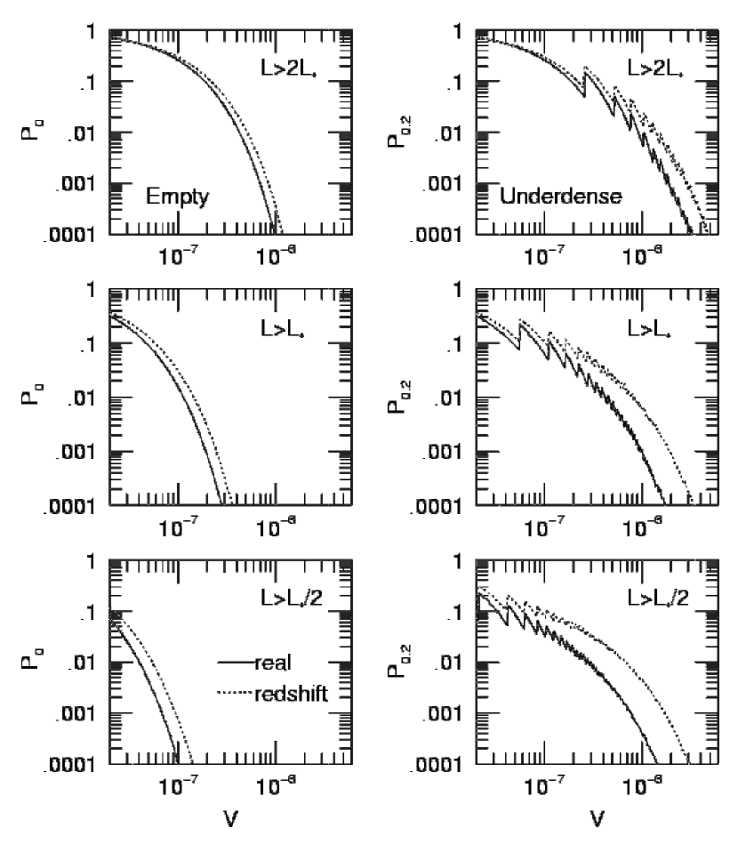
Figure 2: The void probability function (left column) and underdense probability function (right column) for the CDM simulation. In each column, the top panel represents the most sparsely sampled subset of points (corresponding to $L>2L_{*}$), and the bottom panel represents the most densely sampled subset of points (corresponding to $L>L_{*}/2$). The volume is given in dimensionless redshift units.

The void probability function, or VPF (White, 1979) has been a widely used statistic for measuring the characteristic size of voids. The VPF $P_{0}(V)$ is defined as the probability that a randomly located sphere of volume $V$ contains no galaxies. The VPF has been applied to numerical simulations (Fry et al., 1989; Einasto et al., 1991; Weinberg & Cole, 1992; Little & Weinberg, 1994; Vogeley et al., 1994; Ghigna et al., 1994, 1996; Colombi, Bouchet, & Hernquist, 1996; Kauffmann, Nusser, & Steinmetz, 1997) and to redshift surveys (Fry et al., 1989; Einasto et al., 1991; Vogeley, Geller, & Huchra, 1991; Vogeley et al., 1994; Ghigna et al., 1996). The VPF for the simulation studied in this paper is given in the left-hand panels of Figure 2. The volumes plotted are in redshift units; to convert to physical units, multiply by $(c/H_{0})^{3}=6.4\times 10^{10}{\rm\,Mpc}^{3}$. In each panel, the solid line shows the VPF in real space, and the dotted line shows the VPF in redshift space. The effect of peculiar velocity distortions is to increase the void probability at a given volume $V$. A comparison of the VPF for the different sampling densities, however, vividly illustrates the very strong dependence of the VPF on the mean interparticle spacing. To illustrate, let’s define a characteristic void volume $V_{\rm VPF}$ as the volume for which $P_{0}(V_{\rm VPF})=0.01$. For a Poisson distribution of points, $P_{0}(V)=\exp(-\nu V)$, where $\nu$ is the mean number density, and thus $V_{\rm VPF}=4.61/\nu$. For our $L>L_{*}/2$ sample, $V_{\rm VPF}=4.0\times 10^{-8}=9.6/\nu$; for our $L>L_{*}$ sample, $V_{\rm VPF}=1.14\times 10^{-7}=10.3/\nu$; and for our sparse $L>2L_{*}$ sample, $V_{\rm VPF}=4.3\times 10^{-7}=8.3/\nu$. Thus, the voids in the simulation are larger than those in a Poisson distribution of equal $\nu$, but it is still approximately true that the characteristic void size (defining voids as totally empty volumes) is proportional to $\nu^{-1}$.

The dependence of characteristic void size on the sample density $\nu$ is reduced if we use the underdense probability function (UPF) to measure the statistics of voids. The UPF $P_{f}(V)$ is defined as the probability that a randomly located sphere of volume $V$ contains a number density of galaxies that is less than $f\nu$, where $0<f<1$, and $\nu$ is the mean number density of galaxies in the sample. (In a flux-limited survey, we can generalize the UPF so that $P_{f}(V)$ is the probability that a sphere of volume $V$ located at a distance $r$ from the origin contains a number density of galaxies that is less than $f\nu(r)$, where $\nu(r)$ is the mean number density of detected galaxies at $r$.) Following previous work (Vogeley, Geller, & Huchra, 1991; Weinberg & Cole, 1992; Ryden & Melott, 1996), we will set our density threshold at $f=0.2$. The UPF for the simulation studied in this paper is given in the right-hand column of Figure 2; in each panel, the solid line shows the UPF in real space and the dotted line shows the UPF in redshift space. Again, the effect of peculiar velocity distortions is to increase the probability of finding a void of volume $V$. For volumes $V<1/(f\nu)$, the UPF and the VPF are identical, since such a small volume can only fall below the density threshold if it contains no galaxies. In general, a sphere of volume $V$ will be underdense if it contains at most $M$ galaxies, where $M={\rm\,int}(f\nu V)$. When $M$ is small, the UPF shows discreteness effects, visible as the sawtooth pattern in Figure 2; the UPF jumps upward whenever $V$ is an integral multiple of $1/(f\nu)$.

The characteristic void size $V_{\rm UPF}$ is defined as the volume for which $P_{0.2}(V_{\rm UPF})=0.01$. (The choice of $P_{0}=0.01$ as the defining probability is somewhat arbitrary; however, because of the rapid decline of $P_{0}$ at large volumes, the exact value of $P_{0}$ is not crucial.) For our dense $L>L_{*}/2$ sample, $V_{\rm UPF}=2.7\times 10^{-7}=64/\nu$; for the $L>L_{*}$ sample, $V_{\rm UPF}=4.2\times 10^{-7}=38/\nu$; for the sparse $L>2L_{*}$ sample, $V_{\rm UPF}=9.2\times 10^{-7}=17.7/\nu$. The inclusion of peculiar velocity distortions increases $V_{\rm UPF}$ by a factor which ranges from $2.5$ for the densest sample to $1.4$ for the sparsest sample. Although the dependence of the underdense void size $V_{\rm UPF}$ on $\nu$ is less strong than that of $V_{\rm VPF}$, it is not true that $V_{\rm UPF}$ is independent of $\nu$ for plausible sampling densities. Thus, in a flux-limited survey, where the measured $\nu$ decreases with distance from the origin, the characteristic void size $V_{\rm UPF}$ will increase with distance.

4 Void-detection Algorithms

The UPF gives a statistical measure of the number and size of voids in a given galaxy distribution. Frequently, however, it is useful to identify individual voids instead of simply giving a statistical description. Many different algorithms have been used to detect and identify individual voids (Kauffmann & Fairall, 1991; Kauffmann & Melott, 1992; Ryden, 1995; Ryden & Melott, 1996; El-Ad & Piran, 1997; Aikio & Mähönen, 1998). In this paper, we will investigate two void-detection algorithms that are distinguished by their ease of use and clarity of conception. The first algorithm, based on that of Ryden (1995), identifies voids as nonoverlapping spheres; we will call this the “sphere algorithm”. The second algorithm, based on that of Aikio and Mähon̈en (1998; AM) permits voids to be nonspherical; we will call this the “AM algorithm”.

Both void-detection algorithms start by defining a continuous scalar field $D_{f}({\vec{x}})$ within the galaxy survey. At any location $\vec{x}$, $D_{f}$ is defined as the radius of the largest sphere centered on $\vec{x}$ within which the average galaxy density is equal to $f\nu$. To implement the “sphere algorithm”, first locate the global maximum of $D_{f}$ within the survey; call the location of this maximum ${\vec{x}}_{1}$. This is the center of the largest spherical void in the sample, which has a radius $D_{f}({\vec{x}}_{1})$. To find the second largest void, find the point ${\vec{x}}_{2}$ for which $D_{f}$ is maximized, subject to the constraint that

$$D_{f}({\vec{x}}_{2})+D_{f}({\vec{x}}_{1})\geq|{\vec{x}}_{2}-{\vec{x}}_{1}|\ .$$ (1)

The point ${\vec{x}}_{2}$ is then the center of the second-largest spherical void, which has radius $D_{f}({\vec{x}}_{2})$. In other words, the second-largest void is the largest underdense sphere that doesn’t overlap the largest void. Additional voids are found by an iterative process. The $N^{\rm th}$ largest void is located at the position ${\vec{x}}_{N}$ for which $D_{f}$ is maximized, subject to the constraint that

$$D_{f}({\vec{x}}_{N})+D_{f}({\vec{x}}_{i})\geq|{\vec{x}}_{N}-{\vec{x}}_{i}|\ ,$$ (2)

for $i=1,2,\dots,N-1$.

In practice, we compute the values of $D_{f}$ on a cartesian grid superimposed on the galaxy distribution. For the simulation used in this paper, the grid spacing we used was $\Delta x=0.0012$ in redshift units ($\Delta x=4.8{\rm\,Mpc}$ in physical units). This is 0.8 times the resolution of the original numerical simulation. Using a grid very much finer than that of the original simulation is pointless, since there is no information on such small scales. The computed value of $D_{f}$ for each grid point was forbidden to be larger than the distance from the grid point to the sample boundary at z=0.12. We then located the spherical voids, using the algorithm outlined above, subject to the additional constraint that the void centers lie on grid points. Since the discreteness of the superimposed grid creates errors of order $\Delta x$ in the location of void centers, we halt the void-detection algorithm when $D_{f}=2\Delta x$.

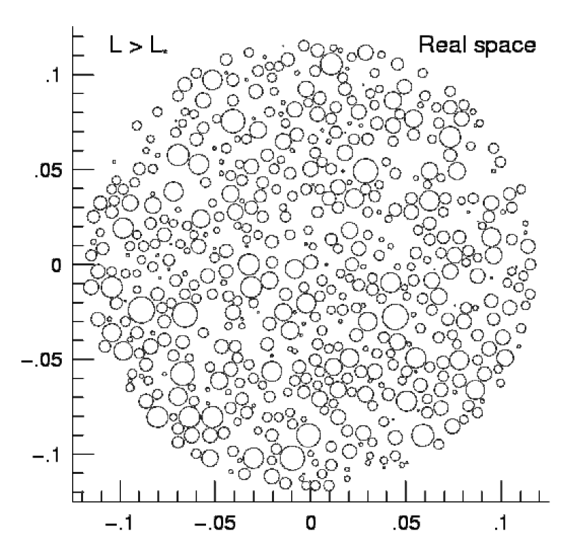
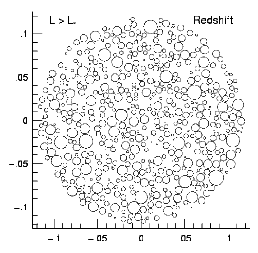
Figure 3: (a) A slice through the spherical underdense voids found in the $L>L_{*}$ sample; the density threshold chosen was $f=0.2$. The orientation of the slice is the same as that shown in Figure 1a. (b) A slice through the spherical underdense voids in the same sample, but with peculiar velocities added.

To emphasize the difference between the properties of totally empty voids and underdense voids, we implemented the sphere algorithm twice, once with $f=0$, and once with $f=0.2$. To illustrate the voids found with the sphere algorithm, Figure 3 shows a slice through the underdense spheres found in the $L>L_{*}$ sample, setting $f=0.2$. Figure 3a shows the spherical voids found in real space (without peculiar velocity distortions) and Figure 3b shows the spherical voids found in redshift space (with peculiar velocity distortions).

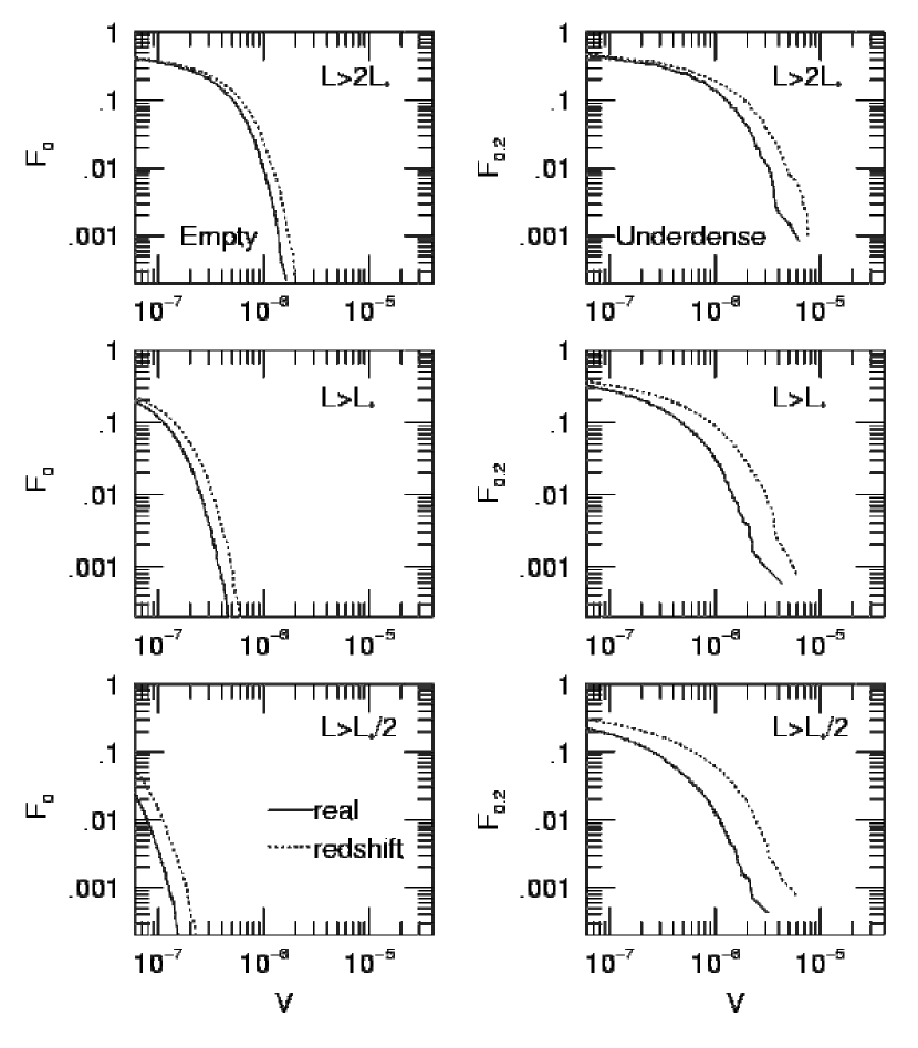
Figure 4: Fraction of the total area of the simulation contained in spherical voids of volume $V$ or greater. In the left column, the density threshold is $f=0$, corresponding to totally empty voids. In the right column, the density threshold is $f=0.2$. In each panel, the solid line is the void fraction measured in real space, and the dotted line is the void fraction measured in redshift space.

To show the spectrum of void sizes found with the sphere algorithm, Figure 4 plots $F_{f}(V)$, the fraction of the total volume of the sample found in spherical voids with volume $\geq V$. The right column of Figure 4 displays $F_{0.2}$, the fraction of the total volume found in voids with underdensity $f=0.2$. For comparison, the left column of Figure 4 gives $F_{0}$, the fraction of the total volume found in totally empty voids. The solid line in each panel gives the distribution in real space, and the dotted line gives the distribution in redshift space. The left column of Figure 4 demonstrates, as in the case of the VPF, that the characteristic size of empty voids depends strongly on the density $\nu$ of the sample. Because of this undesired feature, we will only examine in detail the properties of underdense voids.

A characteristic void size can be found, following the practice of Kauffmann & Melott (1992), by computing the volume-weighted mean void size,

$$\overline{V}=\sum_{1}^{N_{V}}V_{i}^{2}/\sum_{1}^{N_{V}}V_{i}\ ,$$ (3)

where $V_{i}$ is the volume of the $i^{\rm th}$ largest void, and the total number of voids is $N_{V}$. Alternatively, we can define a characteristic void size $V_{X}$ which is the void volume such that $X$ percent of the total volume in the sample is contained in voids of size $V_{X}$ or bigger. The characteristic void sizes $\overline{V}$ and $V_{20}$ are given in Table 1 for underdense voids in samples of different number density, with and without peculiar velocities.

The characteristic size of spherical voids (whether defined as $\overline{V}$ or $V_{20}$) increases in going from real space to redshift space. The more densely sampled the survey, the greater the increase in void size. For the $L>2L_{*}$ sample, $\overline{V}$ increases by 43% in going from real space to redshift space, and $V_{20}$ increases by 40%. For the $L>L_{*}/2$ sample, $\overline{V}$ increases by 88% in going from real space to redshift space, and $V_{20}$ by 155%.

Although the sphere algorithm gives a rough estimate of the spectrum of void sizes, the volumes of the voids found by this algorithm will generally be underestimates of the “true” void size. That is, if a sample contains an empty region surrounded by a continuous, well-defined, extremely overdense wall, the void found by the sphere algorithm will be the largest sphere that can be inscribed within the wall. The remaining empty space within the void wall will then be iteratively filled with smaller and smaller spheres. A more flexible algorithm – one which doesn’t impose the artificial constraint that voids are spherical – should give a more accurate measure of void size.

In addition to underestimating the size of voids, the sphere algorithm gives no hint of the true void shape. In two dimensions, Ryden (1995) and Ryden & Melott (1996) estimated the shapes of voids by fitting ellipses to the underdense region. Each void was then characterized by an axis ratio $q$ and a position angle $\phi$ in addition to its area $a$ and position $(x,y)$. Extending this algorithm to three dimensions by fitting ellipsoids to the underdense regions becomes a computationally daunting task. Each ellipsoidal void must be characterized by two axis ratios and three Euler angles in addition to its volume $V$ and position $(x,y,z)$. The introduction of additional parameters makes the search through parameter space far more time-consuming. Thus, instead of approximating the shape of voids by fitting ellipsoids to them, we adopted the more flexible scheme of Aikio & Mahönën (1998; AM).

To implement the AM algorithm, we start with the field $D_{f}$ as defined on the cartesian grid that we have superimposed on the galaxy survey. If the grid spacing is $\Delta x$, then each grid point can be thought of as being at the center of a cubical “elementary cell” of volume $(\Delta x)^{3}$. We identify the local maxima of $D_{f}$ on the grid as being those points which have values of $D_{f}$ greater than that of their 26 closest neighbors (the 6 points at a distance $\Delta x$, the 12 points at a distance $\sqrt{2}\Delta x$, and the 8 points at a distance $\sqrt{3}\Delta x$). We label the local maxima we find as $M_{1}$, $M_{2}$, $\dots$, $M_{N}$, where $N$ is the total number of maxima located. The AM algorithm assigns every elementary cell to a “subvoid” associated with some maximum $M_{i}$. To discover which subvoid a particular elementary cell belongs to, a “climbing algorithm” is used. For a elementary cell $X$, we compute the gradient in $D_{f}$ to each of the neighboring cells. We then “climb” to elementary cell $X^{\prime}$ for which the gradient has the largest (positive) value. The climbing continues from cell to cell until a local maximum $M_{i}$ is reached. The cell $X$ (and every other cell along the climbing route) is then assigned to the subvoid of maximum $M_{i}$. In this way, every elementary cell is assigned to a subvoid, and each maximum $M_{i}$ has an associated subvoid which consists of at least one elementary cell. Once every elementary cell is assigned to a subvoid, the subvoids are joined together into larger voids. The subvoids associated with maxima $M_{i}$ and $M_{j}$ are members of the same void if the distance between $M_{i}$ and $M_{j}$ is less than both $D_{f}(M_{i})$ and $D_{f}(M_{j})$. Using this criterion, all the subvoids are grouped into voids; some voids contain a single subvoid, while others contain many subvoids linked together in a friends-of-friends percolation. The AM algorithm and its implementation is described in more detail in the original paper by Aikio & Mähönen (1998); our modification is to use the underdensity field $D_{f}$, where AM restricted themselves to the case $f=0$.

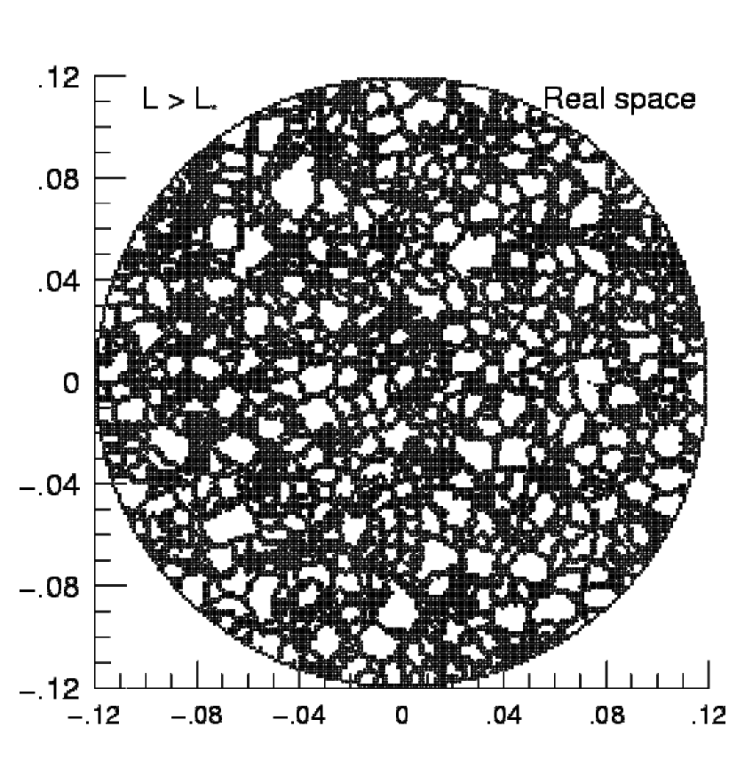
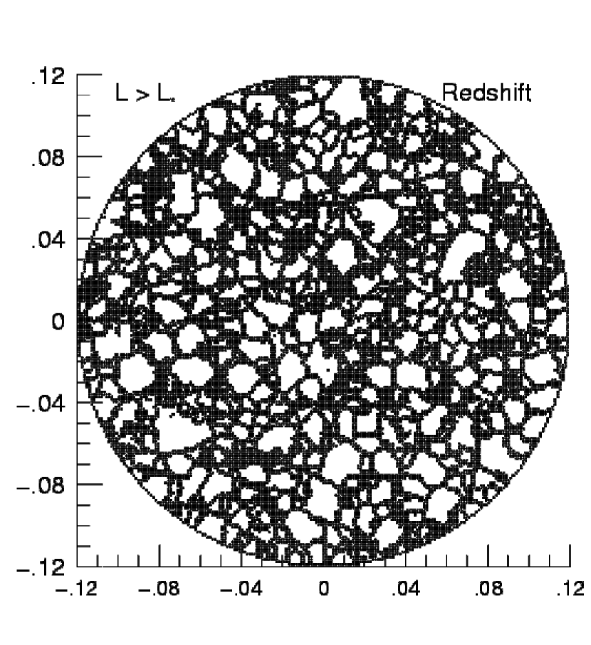
Figure 5: (a) A slice through the underdense voids found in the $L>L_{*}$ sample, using the AM algorithm; the density threshold chosen was $f=0.2$. The orientation of the slice is the same as those in Figures 1a and 3a. (b) A slice through the underdense AM voids in the same sample, but with peculiar velocities added.

Figure 5a shows a slice through the underdense voids in the $L>L_{*}$ sample, without the inclusion of peculiar velocity distortions. The AM algorithm was used with a density threshold $f=0.2$. In each panel of Figure 5, an elementary cell is colored white if it belongs to the same void as its 26 nearest neighboring cells; it is colored black if one or more of its neighbors belongs to a different void. Figure 5b shows a slice through the underdense voids in the $L>L_{*}$ sample, this time with the effects of peculiar velocities included.

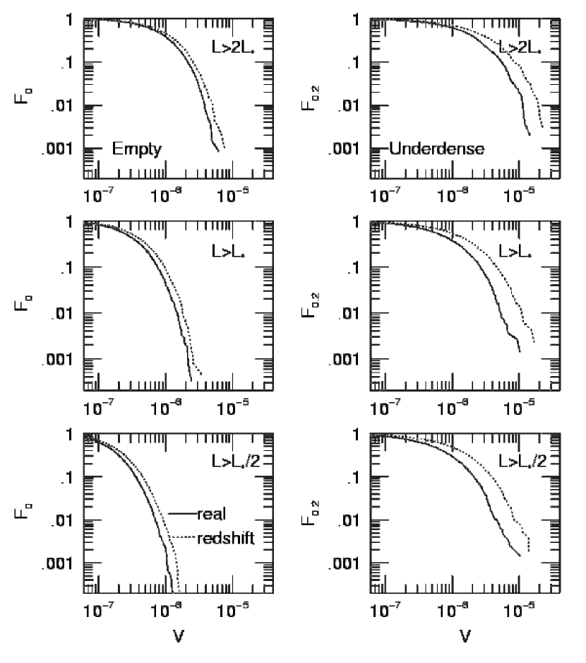
Figure 6: Fraction of the total area of the simulation contained in voids of volume $V$ or greater, as defined by the AM algorithm. In the left column, the density threshold is $f=0$. In the right column, the density threshold is $f=0.2$. In each panel, the solid line is the void fraction measured in real space, and the dotted line is the void fraction measured in redshift space.

The volume $V$ of an individual void found by the AM algorithm can be found by simply adding together the volume $(\Delta x)^{3}$ of the elementary cells which it contains. The full spectrum of void sizes in a particular galaxy sample is given by $F_{f}(V)$, the fraction of the total volume of the sample found in voids with volume $\geq V$. The left column of Figure 6 shows $F_{0}$, the distribution of void volumes using the original algorithm of AM, in which $f=0$. The right column of Figure 6 displays $F_{0.2}$, using our usual underdense criterion, $f=0.2$. Some properties of the AM voids are the similar to those of the spherical voids found earlier. For instance, the left column of Figure 6 shows that the characteristic size of empty AM voids (just like those of spherical voids) is strongly dependent on the density $\nu$ of the sample. Also, peculiar velocities increase the characteristic size of AM voids as well as of spherical voids. Using the AM algorithm with $f=0.2$, the volume-weighted mean void size $\overline{V}$ and the characteristic size $V_{20}$ are given in Table 1. For the sparsely sampled survey ($L>2L_{*}$), $\overline{V}$ increases by 58% in going from real space to redshift space, and $V_{20}$ increases by 66%. For the densely sampled survey ($L>L_{*}/2$), $\overline{V}$ increases by 79% in going from real space to redshift space, and $V_{20}$ increases by 82%. In addition, AM voids as well as spherical voids are larger at lower sampling densities. Given a density threshold of $f=0.2$, the characteristic void size (either $\overline{V}$ or $V_{20}$) for the sparsely sampled survey ($L>2L_{*}$) is 2.5 times that of the densely sampled survey ($L>L_{*}/2$).

One important difference between the voids found by the AM algorithm and those found by the sphere algorithm is that the AM voids are larger. At all sampling densities, it is found that $\overline{V}({\rm\,AM})/\overline{V}({\rm\,sphere})\sim 2.7$. The ratio $V_{20}({\rm\,AM})/V_{20}({\rm\,sphere})$ ranges from $\sim 6$ for the $L>2L_{*}$ survey through $\sim 8$ for the $L>L_{*}$ survey to $\sim 14$ for the $L>L_{*}/2$. Thus, the answer to the seemingly innocuous question, “How large is a typical void?” depends not only on the sampling density of the galaxy survey and on whether the survey is done in real space or in redshift space, but also on the void-finding algorithm used and on the definition adopted for the typical void size.

Another important difference between the voids found by the AM algorithm and those found by the sphere algorithm is that the AM voids are not compelled to be spherical. Hence the shapes of the AM voids can be used as a measure of the shape of voids in the galaxy distribution. It is of particular interest to discover whether voids are distorted along the line of sight from the observer at the origin. At relatively small redshifts ($z\lesssim 1$), the dominant source of distortion in redshift maps is the peculiar velocities of galaxies. In examining two-dimensional simulations with power spectra $P\propto k^{n}$, Ryden & Melott (1996) found only a mild tendency for voids to be distorted or compressed along the line of sight. With an $n=2$ power spectrum, the largest voids were slightly elongated along the line of sight; with an $n=0$ spectrum, voids were slightly compressed along the line of sight.

To find whether the AM voids are preferentially elongated or compressed along the line of sight, we begin by computing the moments of the voids. If a void contains $N$ elementary cells, with the center of the $i^{\rm th}$ cell at $(x_{i},y_{i},z_{i})$, the moments of the void can be computed as

$$\overline{x^{\alpha}y^{\beta}z^{\gamma}}={1\over N}\sum_{i=1}^{N}x_{i}^{\alpha}y_{i}^{\beta}z_{i}^{\gamma}\ .$$ (4)

The “center of mass” of the void, weighting all elementary cells equally, is at $(\overline{x},\overline{y},\overline{z})$. For a given void, we can create a new coordinate system, with its origin at $(\overline{x},\overline{y},\overline{z})$, with its $x^{\prime}$ axis passing through the location of the observer, and with its $y^{\prime}$ and $z^{\prime}$ axis perpendicular to the $x^{\prime}$ axis. If we know the coordinates $(x_{i},y_{i},z_{i})$ of a mass element in the old coordinate system (centered on the observer), we can compute the coordinates $(x_{i}^{\prime},y_{i}^{\prime},z_{i}^{\prime})$ in the new coordinate system (centered on the void center).

A dimensionless measure of a void’s elongation or compression along the line of sight is

$$Q\equiv{3\overline{(x^{\prime})^{2}}\over\overline{(x^{\prime})^{2}}+\overline{(y^{\prime})^{2}}+\overline{(z^{\prime})^{2}}}\ .$$ (5)

The quantity $Q$ has some useful properties. Its denominator is independent of the orientation of the coordinate system; it’s simply the mean square distance of all the elementary cells from the void center. For a void of arbitrary shape, the mean value of $Q$, averaged over all viewing angles, is $<\!Q\!>=1$. Thus, for a population of voids oriented randomly with respect to the observer, we expect the average value of $Q$ to be 1. A value $Q>1$ indicates that a void is elongated along the line of sight; a value $Q<1$ indicates that a void is compressed along the line of sight. For any void, in any orientation, $0\leq Q\leq 3$. As an example, consider a triaxial ellipsoid with principal axes of length $a\geq b\geq c$. The maximum value of $Q$ for this ellipsoid occurs when the long axis is aligned with the line of sight from the observer to the ellipsoid’s center. In this case,

$$Q_{\rm max}={3a^{2}\over a^{2}+b^{2}+c^{2}}\geq 1.$$ (6)

The minimum value of $Q$ occurs when the short axis is aligned with the line of sight. In this case,

$$Q_{\rm min}={3c^{2}\over a^{2}+b^{2}+c^{2}}\leq 1.$$ (7)

For the voids found by the AM algorithm, the denominator of $Q$ can be written as

$$\overline{(x^{\prime})^{2}}+\overline{(y^{\prime})^{2}}+\overline{(z^{\prime})^{2}}=\overline{D^{2}}-\overline{D}^{2}\ ,$$ (8)

where

$$\overline{D}^{2}=\overline{x}^{2}+\overline{y}^{2}+\overline{z}^{2}$$ (9)

and

$$\overline{D^{2}}=\overline{x^{2}}+\overline{y^{2}}+\overline{z^{2}}\ .$$ (10)

The numerator can be written as

$$3\overline{(x^{\prime})^{2}}={3\over\overline{D}^{2}}\left[-\overline{D}^{4}+\overline{x}^{2}\overline{x^{2}}+\overline{y}^{2}\overline{y^{2}}+\overline{z}^{2}\overline{z^{2}}+2\overline{x}\,\overline{y}\,\overline{xy}+2\overline{y}\,\overline{z}\,\overline{yz}+2\overline{z}\,\overline{x}\,\overline{zx}\right]\ .$$ (11)

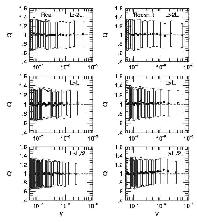
Figure 7: The mean (filled circles) and standard deviation (error bars) for the elongation statistic $Q$; each data point represents a bin containing 400 voids. The left column gives the results for voids measured in real space; the right column gives results for voids measured in redshift space. In each case, the density threshold is $f=0.2$.

To compute the distribution of $Q$ as a function of void volume $V$, we first identify voids using the AM algorithm with a density threshold $f=0.2$; to eliminate distortions caused by the artificial boundary conditions at $z_{\rm max}=0.12$, we consider only those voids at redshifts $z<0.11$. The mean, $\mu_{Q}$, and the standard deviation, $\sigma_{Q}$, of $Q$ for the voids found in this way are plotted in Figure 7, as a function of void volume $V$. The values of $\mu_{Q}$ and $\sigma_{Q}$ are computed in bins containing 400 voids apiece. Thus, the expected error in the mean value of $Q$ for each bin is $\sigma_{\mu}=\sigma_{Q}/\sqrt{400}=0.05\sigma_{Q}$. The value of $\mu_{Q}$ indicates whether voids are preferentially oriented with respect to the line of sight; the value of $\sigma_{Q}$ is a measure of the intrinsic asphericity of the voids.

In the left column of Figure 7, the shape of voids is measured in real space, where there should be no preferential distortions along the line of sight. Indeed, $\mu_{Q}$ is not significantly different from unity for voids of all sizes and at all sampling densities: in all cases, $|\mu_{Q}-1|<2.5\sigma_{\mu}$. There is, however, a significant trend in the standard deviation of $Q$. As voids get larger, $\sigma_{Q}$ gets smaller, decreasing from $\sigma_{Q}\approx 0.34$ at $V=5\times 10^{-8}$ to $\sigma_{Q}\approx 0.27$ at $V>10^{-6}$. This is a consequence of the fact that large voids are more nearly spherical than small voids.

In the right column of Figure 7, the shape of voids is measured in redshift space, where the distortions due to peculiar velocities may cause systematic distortions along the line of sight. At sufficiently high sampling density (the $L>L_{*}$ and $L>L_{*}/2$ samples), large voids are significantly elongated along the line of sight ($\mu_{Q}>1$). In the $L>L_{*}$ sample, $\mu_{Q}>1$ for volumes $V>4\times 10^{-7}\sim 0.2\overline{V}$. In the $L>L_{*}/2$ sample, $\mu_{Q}>1$ for volumes $V>1.3\times 10^{-7}\sim 0.1\overline{V}$; the greatest deviation of $\mu_{Q}$ from unity is at $V=1.25\times 10^{-6}\sim\overline{V}$, where $\mu_{Q}-1=6\sigma_{\mu}$. We conclude that the distortions along the line of sight caused by peculiar velocities are measurable by the AM algorithm only when the sampling density is sufficiently high (corresponding to a limiting galaxy luminosity of $\sim L_{*}$ or fainter). For our initial CDM power spectrum, voids with $V\gtrsim\overline{V}$ show a significant tendency to be elongated along the line of sight by peculiar velocities.

5 Conclusion

In examining the large scale structure of the universe, studies of overdense regions (clusters and superclusters) are usefully complemented by studies of underdense regions, or voids. The properties of voids, such as their volumes and shapes, depend on how voids are defined. Since the literature contains many different void definitions and void-finding algorithms, direct comparison of void properties found in different studies is a risky business.

The VPF, $P_{0}(V)$, depends strongly on the number density $\nu$ of galaxies in the survey. Although the UPF, $P_{0.2}(V)$, depends less strongly on sampling density than the VPF, it is still true that the characteristic void size $V_{UPF}$ depends on the sampling density $\nu$, with a higher density yielding a smaller characteristic void size. Thus, in a flux-limited survey, where the mean density of detected galaxies, $\nu(z)$, decreases with redshift, using a threshold density $f\nu(z)$ will produce a characteristic void size that increases with increasing redshift. This will be an artifact of the decreasing sampling density at large redshift, and does not reflect a change in the underlying large scale structure. In determining how the properties of voids depend on redshift, it is more prudent to extract a volume-limited sample from the data before applying a void statistic like the UPF or a void-finding algorithm.

Of the void-finding algorithms outlined in this paper, the “sphere” algorithm has the virtue of (relative) simplicity. However, its restriction that all voids must be spherical leads to an underestimate of void size and does not permit us to measure the distortions of voids caused by peculiar velocities. Adapting the algorithm of Aikio & Mähönen (1998), we were able to determine more accurately the sizes of underdense voids. As in two-dimensional simulations (Ryden & Melott, 1996), the effect of peculiar velocities is to increase the characteristic void size. The AM algorithm also permits us to measure the elongation of voids along the line of sight. In real space, it is found that large voids are intrinsically more nearly spherical than smaller voids. This can be regarded as a manifestation of the tendency for large voids within a bubbly structure to expand and become more nearly spherical at the expense of their smaller neighbors (Regös & Geller, 1991). In redshift space, large voids are seen, for the CDM spectrum used in our simulations, to have a slight but statistically significant tendency to be elongated along the line of sight. Note, however, that the void distortions can only be detected at a sufficiently high sampling density. Future redshift surveys such as that provided by the Sloan Digital Sky Survey will provide sufficiently high galaxy densities and a large enough number of voids to accurately measure the peculiar velocity distortion of voids in the real universe. When deeper redshift surveys are available, the (relatively small) peculiar velocity distortions can be subtracted out to reveal the cosmological distortions resulting from the deceleration of the Hubble expansion.

Table 1: CHARACTERISTIC VOID SIZES

		Spherical voids		AM voids
Sample		$\overline{V}$	$V_{20}$	$\overline{V}$	$V_{20}$
$L>2L_{*}$	(real)	0.82E-6	0.67E-6	2.26E-6	3.49E-6
	(redshift)	1.17E-6	0.93E-6	3.57E-6	5.80E-6
$L>L_{*}$	(real)	0.42E-6	0.21E-6	1.12E-6	1.75E-6
	(redshift)	0.71E-6	0.39E-6	1.95E-6	3.08E-6
$L>L_{*}/2$	(real)	0.34E-6	0.085E-6	0.91E-6	1.39E-6
	(redshift)	0.64E-6	0.22E-6	1.63E-6	2.53E-6

References

- Aikio & Mähönen (1998) Aikio, J., & Mähönen, P. 1998, ApJ, 497, 534
- Alcock & Paczyński (1979) Alcock, C., & Paczyński, B. 1979, Nature, 281, 358
- Bertschinger (1985) Bertschinger, E. 1985, ApJS, 58, 1
- Blaes, Goldreich, & Villumsen (1990) Blaes, O. M., Goldreich, P. M., & Villumsen, J. V. 1990, ApJ, 361, 331
- Colombi, Bouchet, & Hernquist (1996) Colombi, S., Bouchet, F. R., & Hernquist, L. 1996, ApJ, 465, 14
- Efstathiou, Ellis, & Peterson (1988) Efstathiou, G., Ellis, R. S., & Peterson, B. A. 1988, MNRAS, 232, 431
- Einasto et al. (1991) Einasto, J., Einasto, M., Gramman, M., & Saar, E. 1991, MNRAS, 248, 593
- El-Ad & Piran (1997) El-Ad, H., & Piran, T. 1997, ApJ, 491, 421
- Fillmore & Goldreich (1984) Fillmore, J. A., & Goldreich, P. 1984, ApJ, 281, 9
- Fry et al. (1989) Fry, J. N., Giovanelli, R., Haynes, M. P., Melott, A. L., & Scherrer, R. J. 1989, ApJ, 340, 11
- Fujimoto (1983) Fujimoto, M. 1983, PASJ, 35, 159
- Ghigna et al. (1996) Ghigna, S., Bonometto, S. A., Retzlaff, J., Gottloeber, S., & Murante, G. 1996, ApJ, 489, 40
- Ghigna et al. (1994) Ghigna, S., Borgani, S., Bonometto, S. A., Guzzo, L., Klypin, A., Primack, J. R., Giovanelli, R., & Haynes, M. 1994, ApJ, 437, L71
- Gott, Melott, & Dickinson (1986) Gott, J. R., Melott, A. L., & Dickinson, M. 1986, ApJ, 306, 341
- Icke (1984) Icke, V. 1984, MNRAS, 206, 1P
- Kauffmann & Fairall (1991) Kauffmann, G., & Fairall, A. P. 1991, MNRAS, 248, 313
- Kauffmann & Melott (1992) Kauffmann, G., & Melott, A. L. 1992, ApJ, 393, 415
- Kauffmann, Nusser, & Steinmetz (1997) Kauffmann, G., Nusser, A., & Steinmetz, M. 1997, MNRAS, 286, 795
- Kuhlman, Melott, & Shandarin (1996) Kuhlman, B., Melott, A. L., & Shandarin, S. F. 1996, ApJ, 470, 641
- Lahav et al. (1991) Lahav, O., Rees, M. J., Lilje, P. B., & Primack, J. 1991, MNRAS, 251, 128
- Little & Weinberg (1994) Little, B., & Weinberg, D. 1994, MNRAS, 267, 605
- Melott (1987) Melott, A. L. 1987, MNRAS, 228, 1001
- Melott et al. (1998) Melott, A. L., Coles, P., Feldman, H. A., & Wilhite, B. 1998, ApJ, 496, L85
- Regös & Geller (1991) Regös, E., & Geller, M. 1991, ApJ, 377, 14
- Ryden (1995) Ryden, B. S. 1995, ApJ, 452, 25
- Ryden & Melott (1996) Ryden, B. S., & Melott, A. L. 1996, ApJ, 470, 160
- Sheth (1996) Sheth, R. K. 1996, MNRAS, 278, 101
- Splinter et al. (1998) Splinter, R. J., Melott, A. L., Shandarin, S. F., & Suto, Y. 1998, ApJ, 497, 38
- van de Weygaert & van Kampen (1993) van de Weygaert, R., & van Kampen, E. 1993, MNRAS, 263, 481
- Vogeley, Geller, & Huchra (1991) Vogeley, M. S., Geller, M. J., & Huchra, J. P. 1991, ApJ, 382, 44
- Vogeley et al. (1994) Vogeley, M. S., Geller, M. J., Park, C., & Huchra, J. P. 1994, AJ, 108, 745
- Weinberg (2000) Weinberg, D. H., 2000, private communication
- Weinberg & Cole (1992) Weinberg, D. H., & Cole, S. 1992, MNRAS, 259, 652
- White (1979) White, S. D. M. 1979, MNRAS, 186, 145