Further Adventures: Oxygen Burning in a Convective Shell

Abstract

Two dimensional hydrodynamical simulations of convective oxygen burning shell in the presupernova evolution of a $20\,M_{\odot}\/$ star are extended to later times. We used the VULCAN code to simulate longer evolution times than previously possible. Our results confirm the previous work of Bazàn & Arnett (1998) over their time span (400 s). However, at 1200 s, we could identify a new steady state that is significantly different than the original one dimensional model. There is considerable overshooting at both the top and bottom boundaries of convection zone. Beyond the boundaries, the convective velocity falls off exponentially, with excitation of internal modes. The resulting mixing greatly affect the evolution of the simulations. Connections with other works of simulation of convection, in which such behavior is found in a different context, are discussed.

1. Introduction

There are many published studies of stellar convection using multidimensional hydrodynamical simulations, but few deal with convective nuclear burning occurring in stellar interior (see Deupree (1998) for a study of core hydrogen convection). Arnett (1994) (A94) and Bazàn & Arnett (1994, 1998) (BA94, BA98) have studied oxygen burning shell which is one of the last stages in a massive star presupernova evolution; we extend that work.

This is an important stage in presupernova evolution because in this convective region several phenomena take place. In or near this region: (1) most of the explosive nucleosynthesis and production of ⁵⁶Ni and ⁵⁷Ni occurs, (2) the “mass cut” between collapsed and ejected matter develops, and (3) mixing of different layers may happen. The standard model for treating convection in one dimensional (1D) stellar evolutionary codes, the mixing length theory (MLT), is usually used for modeling this convective region as well, even though the conditions of oxygen convective burning shell are more complicated than can be assumed for MLT to be valid (i.e., the flow is not strongly subsonic and there are both energy sources and sinks in the flow).

In Arnett (1994) this evolutionary stage was described, and the first two dimensional (2D) hydrodynamical simulation of this problem were presented. The 145 s time interval was simulated by these calculations, using the PROMETHEUS code, is much less than the duration of this stage ($10^{3}$ to $10^{5}\rm\ s$, see figures 10.5 and 10.6 in Arnett (1996)). During this time, convective flow was formed. Bazàn & Arnett (1994, 1998) have modeled the evolution over a longer time interval of 300 to 400 s, and noticed a mixing of composition from the neighboring stable region near the end of the simulations. In addition,

• the flow velocities were up to $10\%-20\%$ of the sound speed,

• stellar structure was not altered significantly, and

• there were strong density and composition fluctuations in both space and time which did not reach a statistical steady state.

The main differences between this work and that of A94, BA94, and BA98 were (1) the use of a different hydrodynamic code, and (2) the simulation of a longer evolution time. The same initial model, equation of state, and nuclear reaction algorithms were used.

Figure 1.— Two dimensional velocity field for: a - 75 s, b - 150 s. The upper boundary of the oxygen shell is presented by the thick solid line in a.

2. The numerical scheme

For this study, we used a version of the hydrodynamical code VULCAN (Livne (1993)). This code uses an algorithm that begins with a hydrodynamic time step, and is completed by a relaxation of the numerical grid, thus giving an Arbitrary Lagrangian Eulerian (ALE) scheme. In the hydrodynamic time step, the Lagrangian hydrodynamic equations in two dimensions are solved explicitly or implicitly, allowing longer time steps to be taken if the flow is strongly subsonic. The mesh relaxation phase is necessary to eliminate distortion of the cells, especially for flow with vorticity. We used a quasi-1D Lagrangian relaxation, in which each radial row of cells kept a constant mass. The code was used by Glasner & Livne (1995) for computing convective novae outbursts, and by Asida & Tuchman (1997) and Asida (2000) to simulate convection in a red giant envelope. One of the adaptation made by Asida (2000) for simularions of convection was the inclusion of Smagorinsky (1963) like sub grid scale mixing (SGSM) model, as was done in many two dimensional and three dimensional numerical studies of convection.

The equation of state and the thermonuclear reactions algorithms were essentially the same as in A94 and BA98. The equation of state was the sum of components for electrons, ions, and radiation. The nuclear reaction network used twelve species for helium, carbon, neon and oxygen burning. Neutrino cooling was included; see the above references for details. The initial model was the same as in A94 and BA98. The computational domain corresponds to a region containing the entire oxygen-burning shell in a star of $20\,M_{\odot}\/$, having an initial metallicity of 0.007 (about one third solar). This shell boundaries are at radii of $3\times 10^{8}\rm cm$ and $3\times 10^{9}\rm cm$ that are equivalent to mass coordinates of $1.4\,M_{\odot}\/$ and $2.4\,M_{\odot}\/$.

We performed several simulations that were different in: the computational domain, spacial resolution, the initial temperature gradient and numerical parameters of the simulation. The computational domain typically includes all of the oxygen shell as well as the neighboring layers (the inner radius was located at $2\times 10^{8}\rm cm$ in some of the simulations, and the outer radius was located at $8\times 10^{10}\rm cm$ in other simulations). The angular extent of the wedge ran usually from 0.35 $\pi$ to 0.65 $\pi$ radians.

Typically. the oxygent shell was divided to $\sim$ 120 radial zones, and the spacing of zones was logarithmic in radius and linear in angular direction (i.e., $dr=r\ d\theta$) with 60 angular zones. Rotational symmetry was assumed. These characteristics are similar to the medium resolution simulations of BA98. Because of small differences in the equation of state in the initial one dimensional model and in the two dimensional code, as well as different radial zoning, we had two sets of simulations: in the first, the 1D model (with interpolation) was used as it is, and in the second it was slightly adapted, so that the temperature gradient would be superadiabatic in all zones of the convection shell.

The velocities on the inner boundary were set to be zero for the whole simulation, so that the inner core was a hard sphere. At the upper boundary there was no limitation on the velocities, but in order to eliminate mass flow out of the computational domain, an average radius was used to follow expansion or shrinking of the outer boundary. We used reflective boundary conditions on the sides (though such conditions enforce a downflow or upflow on the side boundaries, it was found in BA98 not to be important).

3. Results of the simulations

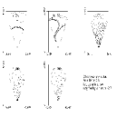
Figure 2.— Carbon abundance contours for: a - 75 s, b - 150 s, c - 300 s, d - 600 s, e - 1200 s.

We present the results of one “standard” simulation with 172 radial zones and 60 angular zones. The inner boundary was at $2\times 10^{8}\rm cm$ and the outer was at $48\times 10^{8}\rm cm$. The temperature gradient was slightly super adiabatic in the oxygen shell, and no SGSM terms were used. Most of the results of the other simulations were similar and the differences are discussed mainly in the end of this section.

3.1. General Evolution of the Flow

In our simulations, the initial velocities were zero, and the convective flow developed as a result of the instability from round off errors. Figure 1 presents the velocity field in the beginning of the simulations for times (a) 75 s and 150 s. As we can see, the convective flow starts at the bottom of the convection region (i.e., the burning layer), and then moves up with increasing eddy size. By time 150 seconds the convective flow penetrates the upper boundary of the convection region (seen as a thick line in panel a). As a result, there is a downflow of carbon-rich material. This can be seen in Figure 2, which presents contours of carbon nucleon fraction. Panels a-e represent times of 75, 150, 300, 600 and 1200 s. We can see that the downflow (panel b) penetrates the whole convective region, and results in mixing of carbon in this region. From comparison of panels c, d and e we can see that carbon abundance becomes more uniform, as the simulation evolves.

This penetration of carbon is almost identical to that seen by BA98; see their Figure 5. The two independent hydrocodes give consistent results over the whole time spanned (400 seconds) by BA98 simulations. The small difference in the timescale for the carbon penetration is due to the small differences in the extent of the super adiabatic gradient of the initial 1D model (when we used the initial 1D model as it is, without modifying the temperature gradient, we got very similar results with a longer timescale of the penetration).

3.2. Carbon Enrichment

Carbon penetration, as well as other processes in the simulations, can be visualized by examining one dimensional averages of various parameters, which in principle would be equivalent to results from 1D simulations. In Figure 3 carbon abundance (nucleon fraction) is plotted as a function of stellar mass coordinate. From the initial profile (solid line) we can see the location of the oxygen shell. At 150 s (long dashed line), carbon rich material has entered the convection layer, and then mixed through the whole region. At later times, the fluctuations in the abundances of carbon decrease (compare the profiles at 300 s -short dashed line, 600 s - dotted line and 1200 s -dotted dashed line), and we have a carbon nucleon fraction of $\sim 5\times 10^{-3}$.

FIG.  3.— Average carbon abundance

A change in abundance in this plot does not necessarily corresponds to mixing, because this plot represents an one dimensional average of the compositions of all the material in each radial layer. This may be revealed by a closer look at the apparent widening of the jump in carbon abundance at the upper boundary of the oxygen shell at $m\approx$$2.4\,M_{\odot}\/$: this jump is much wider at 150 s than it is at later times. This “anti diffusion” is possible since the widening of the interface of the shell is the outcome of two processes: a mixture of material from the two sides of the interface and large scale motions that change the shape of the interface. Thus, at later times the interface is more spherical than it was at 150 s, so that averaging the abundances over radial layers yields a sharper jump (compare Fig 2 panels b and d).

FIG.  4.— RMS fluctuations of carbon abundance

To better understand the carbon enrichment we present Figure 4 which shows the RMS fluctuations of carbon nucleon fraction ($\sigma$) as a function of stellar mass coordinate at several different times. The tendency toward more uniform carbon mixing is clearly seen, as was indicated by Figures 3 and 4. From this figure, we can also see, that the previously mentioned widening of the oxygen shell interface is partially due to changes in its shape since the fluctuations in carbon fraction at the boundary are relatively high, and are even higher at time 150 s.

FIG.  5.— Nuclear luminosity as a function of time.

The mixing of carbon in the burning layer causes the reaction rate to change significantly. In Figure 5, the nuclear luminosity is presented as a function of time. In the beginning there is an adjustment phase in which the energy production rate decreases to about $5\times 10^{44}\rm\ erg\ s^{-1}$ . This transient phase is a thermal relaxation due to the fact that the initial model is inconsistent: it does not have a two dimensional velocity field which can carry the convective energy flux that the 1D model needed. As the carbon rich material penetrates to high temperature layers, it starts to react rapidly, yielding nuclear luminosities which increase to about hundred times the initial value. In this stage, the result is mainly carbon and neon consumption. Afterward, there is a smaller decrease in nuclear luminosity (compare time 600 and 1200 s). This decrease is related to the small decrease in the average carbon abundance seen between times 600 s and 1200 s in Figure 3.

3.3. A Quasi-Steady State

FIG.  6.— Time average change in energy

The relaxation in the carbon abundances by time 300 s to a slowly varying state, and the small change between times 600 and 1200 s, suggest that the system may be close to a quasi - stationary state (a “steady” state on average). This one is significantly different from the steady state predicted by the one dimensional calculations used to definethe initial model. That the system is close to a steady state can be demonstrated by the following figures. Figure 6 shows the average rate of change in energy, as a function of mass coordinate (from time 400 to time 800 s). The energy produced by thermonuclear reactions (dashed line) is carried away by convection (solid line). The net change in energy is small, and balanced by changes in the gravitational energy (dotted line). This slow change is an adjustment of the structure driven by enhanced nuclear burning from the carbon ingestion. There is a net heating at the bottom, below $1.4\,M_{\odot}\/$, which will be addressed in the next section.

FIG.  7.— Time average change in carbon abundance

Figure 7 shows the average rate of change in carbon nucleon fraction, as a function of mass coordinate (from time 400 s to time 800 s, and from time 800 s to time 1200 s), comparing the changes due to the divergence of the convective abundance flux (solid line) with that due to nuclear burning (long dash line). The nuclear consumption of carbon at the bottom is almost completely balanced by convective inflow; This is the burning zone. Over most of the convection region the change in carbon abundances is small. There are larger fluctuations at the top (outer) boundary of the convection zone (where the carbon abundance increases by a factor of $\sim 20$, see Fig. 3).

The decrease in nuclear luminosity (seen in Figure 5, after the peak at 200 s) was caused by a decrease in the net flux of carbon into the burning layer. This is easily seen in Figure 7 in the comparison of the changes in the later time interval (800 s to 1200 s - short dashed line) to the changes in the previous time interval (400 s to 800 s - solid line). The total mass of carbon in the oxygen convection shell is decreasing as a result of carbon consumption and less mixing from the upper shells. Thus our convective burning is beginning to evolve on a secular time scale by the consumption of fuel, having approached a thermal “steady” state.

in Figure 8 we present the RMS fluctuations of density (divided by the density) as a function of stellar mass coordinate for the standard simulation for several times. As the composition becomes more uniform with time, the density fluctuation decreases throughout most of the oxygen shell to about $10^{-3}$ at time 1200 s. However at the edges of the convection zone, the fluctuations does not decrease and we have about $2\times 10^{-2}$ at the bottom and $7\times 10^{-2}$ at the top, where there is a jump in the abundances. These values are similar to those obtained by BA98.

FIG.  8.— RMS fluctuations of the density

3.4. Interaction with Neighboring Shells

FIG.  9.— Temperature profile at the bottom

One important interaction of the convective shell with neighboring shells is the mixing of carbon from the upper carbon rich shells, as described before. Another important interaction is heating of the nearest shells below the bottom of the convection zone: in the initial model there is a sharp decrease in temperature just below the convection zone, as convective flow starts to grow inside the lower parts of the convection zone there is some penetration of the flow to these lower temperature shells. As a result of this flow, the lower temperature shells are being heated and the higher temperature shells are being cooled. This heating is easily seen in Figure 9 where we present the temperature profile in the initial model, and at later times. Most of the heating was done by time 300 s, but even at later times, some heating exsisted, as can be seen in the left end of Figure 6. Along with this “energy mixing” there is mixing of composition in those few zones as we can see from neutron excess $\eta$ plot presented in Figure 10. In the initial model, there is a jump in $\eta$ at the boundary of the oxygen shell (corresponds to the jump in composition). Due to mixing, this jump slightly moves towards lower mass coordinate and becomes slightly wider. From comparison of Fig. 9 and 10 we see that the heating penetrates to deeper shells than composition changes.

FIG.  10.— Neutron excess $\eta$ at the bottom

There are two important consequences of this interaction: (1) the heating and aditional oxygen and carbon in the few zones below the 1D oxygen convection shell cause these zones to be added to the oxygen shell and, together with few zones at the bottom of it, to be part of the burning zone (we can see a broader region with temperature above $2.2\times 10^{9}\rm cm$), (2) because of the cooling of the zones at the bottom of the oxygen shell, the temperature gradient becomes less than adiabatic in those zones and the convective flow exist as a result of a super adiabatic gradient at higher zones.

FIG.  11.— Convective velocity at the bottom

Thus we see that the neighboring stable shells greatly affect the oxygen convective shell. The same convective flow that penetrates to the neighboring shells and allow the mixing of elements and energy between the shells affects further more the stable shells. In Figure 11 we present the averaged convective velocity as a function of radius at the bottom of the oxygen shell. The dashed line corresponds to the fluctuations in radial component of the velocity, while the solid line corresponds to the amplitude of the fluctuating total velocity. The plus signs present points in which the pressure varies by a factor of ten. Three regions can be identified in this plot from right to left: a region of constant velocity, a region of exponential decrease, and another region of constant velocitis but with a noticeable difference between the total and the radial velocities. (i.e. the radial velocities are much smaller on average than the tangential velocities) which is indicative of g modes. This g modes can be identified in 2D presentation of the flow (Figure 12).

FIG.  12.— Velocity field at the bottom. The thick line represents the composition jump that indicates the boundary of the oxygen shell

In another simulation we included a much larger shell above the oxygen shell. In this simulation we noticed similar flow characteristics of exponential decay (Figure 13) and tangential preference of the flow (Figure 14). From Fig. 11 and 13 we can also see that the exponential decrease at the bottom is on a scale which is about one third of the pressure scale height, while at the top it is over one pressure scale height.

FIG.  13.— Convective velocity at the top

FIG.  14.— Velocity field at the top. The thick line represents the composition jump that indicates the boundary of the oxygen shell

3.5. Numerical Sensitivity

We performed several simulations with different parameters as mentioned in §2. As our results are consistent with those of BA98, and since one of the main subjects in BA98 is the sensitivity of the results to numerical parameters, we would not present here all the results from our many simulations. Instead, we will focus on the conclusions from those simulations: the most sensitive feature in the results is the amount of heating below the oxygen shell. When there is more heating, the temperature gradient is less than adiabatic in a larger portion of the (bottom of) oxygen shell. As a result, the convective flow is damped, carbon can not reach the burning zone and we got less nuclear luminosity.

The opposite happened in simulations where we did not include the shell below the oxygen shell: the temperature gradient was super adiabatic so the velocities were higher (by a factor of five), more carbon entered the burning zone, and the nuclear luminosity was higher. From comparison of simulations with different resolution for this case (without the bottom shell), we found that the results are quite robust and not sensitive to the numerical resolution.

In all of our simulations the other features were essentially the same, namely: the evolution of the flow from the bottom, the penetration to neighboring shells and the enrichment of the oxygen shell by carbon.

FIG.  15.— Extra $\eta$ mixing at the bottom

In order to check extra mixing at scales shorter than numerical resolution, we performed a simulation with SGSM mixing terms. This simulation started from a 2D profile of the standard simulation at time 400 s and was carried out to time 800 s. The differences between this simulation and the standard simulation were: a more uniform composition at the oxygen shell - the RMS fluctuations of carbon abundance at time 800 s were similar to the results of the standard simulation at time 1200 s, and significantly more mixing at the stable bottom shell. This can be seen in Figure 15 were we plot the neutron excess $\eta$ for this simulation (SGSM) and the standard simulation. In this plot we can see a very small difference between the two profiles of the standard simulation (at time 400 s - solid line and at time 800 s - long dashed line). When SGSM terms were added, more mixing can be seen by time 600 s (short dashed line), and additional mixing occurs until the end of the simulation (time 800 s - dotted line).

4. Discussion

When we compare our results to the results of BA98 we note that the evolution of the simulations is similar for times reached previously. In both, convective flow evolves from bottom to top, with velocities exceeding $10\%$ of the sound speed. The flow penetrates to the carbon rich region above the one dimensional edge of the convective region, and thus causes a significant enrichment of the convective region with carbon. These higher values of carbon abundances yield a much higher nuclear luminosity than did the original oxygen burning.

However, at later times, we could identify signs of a steady state configuration in which the average abundances changed very slowly, and turbulent mixing within the convective region was able to decrease the fluctuations in the oxygen shell. However, density fluctuations near the boundaries of the convection zone (which are also composition discontinuities) did not decrease at later times, and were equal to few percents.

The most prominent feature in our simulations is the interaction of the convective shell with the neighboring shells. This interaction is due to penetration of the convective flow to the stable shells and the resulting mixing of elements and energy. These effects were present in all of our simulations, and seemed to be physically resonable and valid. However, the exact amount of mixing (especially at the bottom) depends on numerical parameters of the simulations. Moreover, since the initial 1D model did not include such overshoot, we actually simulated a transient toward a more consistent model. For example, we mentioned that the heating of the very few neighboring zones ,at the bottom of the convection shell, lowers the temperature gradient below the adiabatic value. If the convective flow is damped because of that, then the heat generation in these zones would evantually increase the temperature gradient, and convection would be restored.

The properties of the internal modes excited in the stable shells are undoubtedly affected by the computational domain and the boundary condition. Reflective waves are probably the cause for the constant level of velocities we noticed at Figure 11. However, the volume below the oxygen shell in these stars is relatively small so a finite value of the velocity is quite plausible.

An interesting point is the validity of the results as we performed 2D simulations (and not 3D). This is not an easy question to answer, however, from various comparisons of 2D and 3D simulations (see for example Kiraga et al. (1999)) it seems that the main features of the interaction of the unstable layer and its neighboring layers are similar, and the overshoot and mixingin in both cases are comparable . As we do not claim to resolve this interaction quantitatively, we think that our results are valid.

Penetration of the convective flow to neighboring stable regions is a common feature that exists in many multidimensional simulations of convection, in a variety of stellar problems. Hurlburt, Toomre, & Massaguer (1986) have studied such penetration beyond a shallow convective region in 2D, and found that it generated internal g modes in the stable region below the convection region, all the way to the bottom boundary. Two regions in this stable layer can be identified from their figure 13: close to the unstable layer there is a sharp decrease in the kinetic energy, but it does not go to zero, rather there is an almost constant level of kinetic energy throughout the rest of the stable layer. Kiraga et al. (1999) have tested penetration in both 2D and 3D, they found that the energy fluxes in the stable layer in the 3D are about two thirds of the 2D results and that the constant level is replaced with a continuas decrease when the viscosity coefficient is increased at the bottom to avoid reflection of waves.

In both these studies, ideal simplified physics was assumed. Freytag, Ludwig, & Steffen (1996) studied the structure and dynamics of shallow stellar surface convection zones, using two dimensional radiation hydrodynamic simulations with more “real” physics. They found convective motions extending “well beyond the boundary of convectively unstable region, with vertical velocities decaying exponentially with depth in the deeper parts of the lower overshoot region, as expected for linear $g^{-}$ modes.” They suggested to approximate the average velocity at the stable region as the convective velocity at the boundary of the unstable zone multiplied by an exponential decay factor with a lapse rate that is of order of the pressure scale height.

As explained by Cox (1980, §17.8) g^- modes are unstable within convection regions, and generally decrease exponentially with increasing distance from the boundaries of the oscillatory region. As Freytag, Ludwig, & Steffen (1996) point out, Landau & Lifshitz (1959) have a relevant discussion in their §34, where they discuss some properties of potential flow. If compressibility and dissipation can be neglected, a steady state potential flow which is periodic in some plane, must be damped exponentially in a direction perpendicular to that plane. Also, the shortest wavelengths will be damped fastest. Consequently, most of the overshoot is given by the largest scales which are driven at the interface, that is, the largest convective scale.

We find a striking underlying unity in these results and ours, despite the significantly different astrophysical context involved: our simulations correspond to deep shell burning convection that is driven by nuclear burning at the bottom and cooled by neutrino radiation and in which spherical properties of the domain are important; while these studies deal with envelope convection driven by photon radiation at the surface in plane parallel geometry. In both cases The flow extand beyond the formal boundaries of the convection zone, with velocities that decay exponentially in the stable shells producing internal modes.

Near the boundaries of the convection zone, where the velocities are still large, quite efficient mixing is taking place. The amount of mixing beyond that region, is not entirely clear. Freytag, Ludwig, & Steffen (1996) have used trajectories of test particles to estimate the diffusion coefficient and conclude that the diffusion coefficient corresponds directly to the exponentially decaying velocities.

Some studies of stellar evolution that used these mixing terms for hydrogen core convection (Herwig et al. (1997); Herwig et al. 1998), found that the lapse rate of decay of the diffusion should be much smaller ($\approx$2 percents) than the pressure scale height. They speculate that this is due to the large stability of the layers that are near the core convection zone. Yet another explanation might be true, namely the flow characters at the stable shells and the many scales involved in mixing.

Mixing is a complex phenomenon which take place in a very small length scale comparing to the length scale of the star, and since stars have a lower effective viscosity than in the simulations, and since they evolve for longer times, an accurate prediction of mixing is very difficult. Further, we note that motion does not necessarily imply mixing! In particular, oscillatory potential flow, which is irrotational,would involve “stretching” and “contracting” motions that do not give mixing, at least at lowest order.

As we can see in Figures 11-14, The flow in the stable shells is different than the flow inside the convection region, even though it is not purely potential flow (as revealed when examining the vorticity). Due to these differences in the flow, it seems plausible that the effective mixing velocity may be less than the hydrodynamic velocity, and its lapse rate different as well.

As the various shells in our model have a different composition, mixing can be directly examined from the 2D profiles and the 1D average of composition. However, as the scale of mixing is much smaller than numerical resolution, the results must be carefully examined. One way to examine the results is to compare the mixing in the standard simulation to that in the simulation with sub grid mixing model. There are small differences in the average abundances in the oxygen shell between the two simulations, and the main difference is that with SGSM terms, the profile is more uniform because of the extra mixing. The difference between the simulations is much more prominent in the lower stable shell: the width of the abundance jump is much wider when SGSM terms were used, and penetrates to deeper zones, in which the “constant level” average velocity exists.

When we used SGSM we implicitly assumed that turbulent flow exists from the scale of the mesh resolution to the scale of molecular diffusion. Since this mixing occurs in a stable region, in which internal modes have been excited, the validity of this assumption is questionable. Thus it is fair to say that further work is needed to resolve this subject of mixing beyond the convective layers.

Mazzitelli, D’Antona, & Ventura (1999) have examined the effects of overshooting predicted by full spectrum turbulence model of convection (Canuto & Mazzitelli 1991, 1992) within the context of lithium production in AGB stars. This is an interesting example of the way stellar convection may be tested. A particular aspect of their work of interest here is the suggestion that symmetric overshoot may be constrained by existing observations. We note that a general feature of numerical simmulations is up-down asymmetry. Cooling flows are narrow, faster downdrafts than the corresponding updrafts, which are broader and slower. It is suggestive that in simulations of envelope convection driven by radiative cooling at the top, there is an overshoot at the bottom (Hurlburt, Toomre, & Massaguer (1986); Freytag, Ludwig, & Steffen (1996)), while we, who have simulated shell convection driven by burning at the bottom, have found exponential overshoot at the top (and the bottom). It may be that the causes of this asymmetry can be determined, so that a complete algorithm for the overshoot maybe devised for 1D stellar evolutionary calculations.

In summary, we found that stellar evolution models should take into account penetration and an exponential decay of the velocities, and the excitation of internal modes, when simulating convective burning shells. Direct hydrodynamic simulation of stellar evolution places heavy demands on computer resources, especially for carbon and neon burning stages, which are slower. The tendency toward steady state revealed in our simulations is encouraging in that simplified algorithms may allow the construction of an improved set of one dimensional models.

We used an initial model which was derived from results of a one dimensional stellar evolution code, in which earlear stages of evolution were modeled with standard MLT. Consequently, the profile we started with is unsatisfactory, and is not consistent with our conclusion that penetration and extra mixing should be taken into account. This should be kept in mind when using directly the results of our simulations.

References

- Arnett (1994) Arnett, D. 1994 ApJ, 427, 932
- Arnett (1996) Arnett, D. 1996, Supernovae and Nucleosynthesis (Princeton, New Jersy: Princeton University Press)
- Asida (2000) Asida, S.M. 2000 ApJ, 528, 896
- Asida & Tuchman (1997) Asida, S.M., & Tuchman, Y. 1997 ApJ, 491, L47
- Bazàn & Arnett (1994) Bazàn, G., & Arnett, D. 1994, ApJ, 433, L41
- Bazàn & Arnett (1998) Bazàn, G., & Arnett, D. 1998, ApJ, 496, 316
- Canuto & Mazzitelli (1991) Canuto, V. M., & Mazzitelli, I. 1991, ApJ, 370, 295
- Canuto & Mazzitelli (1992) Canuto, V. M., & Mazzitelli, I. 1992, ApJ, 389, 724
- Cox (1980, §17.8) Cox, J.P. 1980, Theory of Stellar Pulsation (Princeton, New Jersy: Princeton University Press)
- Deupree (1998) Deupree, R. G. 1998, ApJ, 499, 340
- Freytag, Ludwig, & Steffen (1996) Freytag, B., Ludwig, H. -G, & Steffen, M. 1996, A&A, 313, 497
- Glasner & Livne (1995) Glasner, S. A., & Livne, E. 1995, ApJ, 445, L149
- Herwig et al. (1997) Herwig, F., Blöecker, T., Schöenberner, D., & El Eid, M. 1997, A&A, 324, L81
- Herwig, Schöenberner, & Blöecker (1998) Herwig, F., Schöenberner, D., & Blöecker, T. 1998, A&A, 340, L43
- Hurlburt, Toomre, & Massaguer (1986) Hurlburt, N.E., Toomre, J., & Massaguer, J.M. 1986, ApJ, 311, 563
- Kiraga et al. (1999) Kiraga, M., Zahn, J.-P., Stȩpień, K., Jahn, K., Rózyczka, M. & Muthsam, H. J. 1999, in ASP Conf. Ser. 173, Theory and Test of Convection in Stellar Structure, ed. Á. Giménez, E. Guinan, B. Montesinos (San Francisco: ASP), 269
- Landau & Lifshitz (1959) Landau, L. D., & Lifshitz, E. M., 1959, Fluid Mechanics (London: Pergamon Press)
- Livne (1993) Livne, E. 1993, ApJ, 412, 634