Limits on Cosmic Matter–Antimatter Domains from Big Bang Nucleosynthesis

Abstract

We present detailed numerical calculations of the light element abundances synthesized in a Universe consisting of matter- and antimatter- domains, as predicted to arise in some electroweak baryogenesis scenarios. In our simulations all relevant physical effects, such as baryon-antibaryon annihilations, production of secondary particles during annihilations, baryon diffusion, and hydrodynamic processes are coupled to the nuclear reaction network. We identify two dominant effects, according to the typical spatial dimensions of the domains. Small antimatter domains are dissipated via neutron diffusion prior to ⁴He synthesis at ${T_{{}^{4}{\rm He}}}\approx 80$ keV, leading to a suppression of the primordial ⁴He mass fraction. Larger domains are dissipated below ${T_{{}^{4}{\rm He}}}$ via a combination of proton diffusion and hydrodynamic expansion. In this case the strongest effects on the elemental abundances are due to $\bar{p}$⁴He annihilations, leading to an overproduction of ³He relative to ²H and to overproduction of ⁶Li via non-thermal nuclear reactions. Both effects may result in light element abundances deviating substantially from the standard Big Bang Nucleosynthesis yields and from the observationally inferred values. This allows us to derive stringent constraints on the antimatter parameters. For some combinations of the parameters, one may obtain both, low ²H and low ⁴He, at a common value of the cosmic baryon density, a result seemingly favored by current observational data.

]

I Introduction

Recently, there has been a revived interest in antimatter cosmologies, stimulated in part by the first flight of the Alpha Magnetic Spectrometer (AMS) and by the prospect of a long-term AMS mission on board of the International Space Station Alpha (ISSA). While these efforts concentrate on direct detection of antinuclei in the solar system, several limits on the existence of antimatter domains have been placed in the past. It has been known for a long time, that the presence of significant amounts of antimatter within a distance of about 20 Mpc from the solar system may be excluded on grounds of the non-observation of annihilation radiation [1]. More recent studies of the diffuse $\gamma$-ray background claim to exclude antimatter regions in today’s Universe within a distance of $\sim$ 1000 Mpc [2], a considerable fraction of the present horizon $\sim 3000\,$Mpc. The existence of antimatter domains would also have impact on the Cosmic Microwave Background Radiation (CMBR). Recent studies predict ‘ribbon’- or ‘scar’-like anisotropies in the CMBR, at the interfaces of matter- and antimatter domains, with a Sunyaev-Zel’dovich-type $y$ distortion of the order of $10^{-6}$ [3, 4]. Such small distortions are beyond the detection limits of current CMBR observations, and probably also beyond those of the upcoming MAP and PLANCK satellite missions. Given that only a small region of the parameter space for the sizes of antimatter domains remains, it seems very unlikely that we live in a Universe containing any considerable amount of antimatter today. In particular, the possibility of a baryo-symmetric Universe containing equal amounts of matter and antimatter is excluded unless the separation length of matter and antimatter is nearly as large as the current horizon. It is, however, not possible on grounds of the above results to exclude the existence of small and distant pockets of antimatter [5].

A complementary scenario with small scale domains of antimatter which have completely annihilated prior to recombination has, however, hardly been investigated in the past. Note that such a scenario necessarily involves an excess of matter over antimatter. While the very precise observation of the CMBR allows us to place stringent limits on any non-thermal energy input into the CMBR during epochs with CMBR temperature $0.3\,{\rm eV}\lesssim$ $T\lesssim 1\,$ keV, in particular, also on energy input due to annihilations [6], even more stringent constraints may be derived from considerations of Big Bang Nucleosynthesis (BBN, hereafter). Such a baryo-asymmetric Universe filled with a distribution of small-scale regions of matter or antimatter may, for example, arise during an epoch of baryogenesis at the electroweak scale. It has been shown within the minimal supersymmetric standard model, and under the assumption of explicit as well as spontaneous $CP$ violation, that during a first-order electroweak phase transition the baryogenesis process may result in individual bubbles containing either net baryon number, or net anti-baryon number[7]. More recently, it has been argued that pre-existing stochastic (hyper)magnetic fields in the early Universe, in conjunction with an era of electroweak baryogenesis, may also cause the production of regions containing either matter or antimatter [8]. Though it seems questionable at present if electroweak baryogenesis has occurred at all, there are other imaginable scenarios which could lead to a small-scale matter-antimatter domain structure in the early Universe [9].

This kind of initial conditions may have profound consequences on the abundances of the cosmological synthesized light elements. In the standard picture, synthesis of the light elements takes place between the cosmological epoch of weak freeze out at $T\approx 1$ MeV and $T\approx 20$ keV. The abundances of the light elements are highly sensitive to the cosmic conditions during that epoch. For example, the primordially synthesized ⁴He mass fraction is sensitively dependent on the relative abundances of protons and neutrons at ${T_{{}^{4}{\rm He}}}\approx 80$ keV, when practically all available neutrons are incorporated into ⁴He nuclei. We have recently shown that annihilation of antimatter domains during BBN (at temperatures above ${T_{{}^{4}{\rm He}}}$) may significantly alter the neutron-to-proton ratio at ${T_{{}^{4}{\rm He}}}$ [10]. However, light element abundances are also sensitive to putative matter-antimatter annihilations after the epoch of BBN. In this paper, we thus extend our analysis of annihilation of antimatter domains to a much wider temperature regime, from above the epoch of weak freeze out to the epoch of recombination. This allows us to constrain matter-antimatter domains within a much wider range of domain separations. The same scenario, annihilation of matter-antimatter domains during and after BBN, has been very recently investigated in a Letter by Kurki-Suonio and Shivola. [11]. Though the main conclusions of our paper are not vastly different from those of Ref. [11], we arrive at somewhat different results (factor $\sim 3$) for the synthesis of some of the elemental abundances. Furthermore, we use a different approach in comparing our theoretical results with observationally inferred values for the light element abundances. In particular, we base our constraints on observationally determined limits on the primordial ³He/²H ratio, rather than on the much less secure limit on primordial ³He. We also consider the production of ⁶Li which yields a tentatively much more stringent limit on the existence of antimatter domains.

Prior studies of the influence of antimatter domains on the light element abundances have only been carried out in the context of a baryo-symmetric Universe [1, 12]. Of course, such models have to assume that annihilation of all cosmic baryons may be avoided by an assumed “unphysical” , and unknown rapid separation mechanism of matter from antimatter. In essence, these works have shown that antimatter domains and successful BBN mutually exclude each other in baryo-symmetric cosmologies unless the separation between matter and antimatter domains is exceedingly large. In that case, however, BBN proceeds in a standard way, independently in matter and antimatter domains.

There have been a number of studies concerning a homogeneous injection of antimatter into the primordial plasma during, or after BBN [13, 14, 15, 16]. Antibaryon production may result through the decay of relic, heavy particles $X$, if hadronic decay channels are present, or the evaporation of primordial black holes. A possible candidate for the $X$-particle is the gravitino, the superpartner of the graviton. It was realized early that antibaryons injected around weak freeze out would increase the synthesized ⁴He abundance, due to preferential annihilation on protons [17]. This was used to derive a limit on the relative antibaryon abundance of $n_{\bar{b}}/(n_{n}+n_{p})\lesssim 1/20$. Injection of antibaryons after BBN would result in $\bar{p}$⁴He annihilations [13]. The concomitant production of ²H, ³H, and ³He, either by direct production during ⁴He annihilation, or by fusion processes of secondary neutrons, was found to give unacceptable large (²H + ³He)/H, unless $n_{\bar{b}}/n_{b}\lesssim 10^{-3}$ [14]. Such arguments were subsequently used to constrain the abundances of particular relic particles [15]. Motivated by the idea to reconcile a Universe dominated by baryonic dark matter with BBN, Yepes & Domínguez-Tenreiro investigated the effects of antibaryons injected during BBN [16]. An outstanding feature of such scenarios is a significant reduction of ⁷Li production compared to standard BBN. Nevertheless, the claim that such scenarios may be compatible with a fractional contribution of baryons to the critical density of $\Omega_{b}=1$ seems not viable due to the overproduction of ⁴He and the ³He/²H ratio.

In this paper we investigate BBN with matter-antimatter domains. Assumed initial conditions and definitions which are used throughout the paper are introduced in Sec II. In contrast to homogeneous antimatter injection, this topic requires an understanding of hydrodynamic and diffusive processes which lead to the mixing of matter and antimatter. These processes are summarized in Sec. III. Nuclear annihilation reactions and the production of secondaries and their evolution are investigated in Sec. IV. In Sec. V we then present results of detailed numerical simulations of BBN in presence of matter-antimatter domains. New and stringent limits on antimatter domains are derived in Sec. VI, whereas Sec. VII is devoted to discussion and conclusions. The appendices discuss the structure of the actual annihilation region (App. A) and some aspects of the numerical treatment of the problem (App. B).

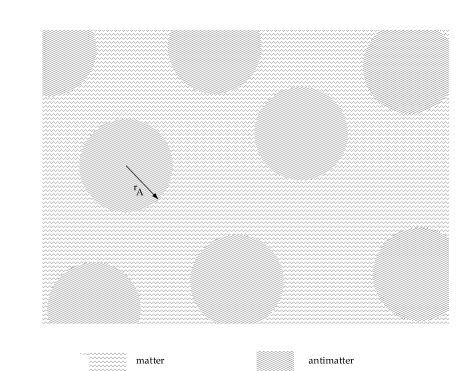
FIG. 1.: Sketch of the assumed initial conditions: Antimatter domains are embedded in a background of matter.

II Preliminaries

In this work, we consider cosmological models which contain different amounts of antimatter distributed in domains of various sizes $r_{\rm A}$. In such scenarios, the Universe may be envisioned as a distribution of matter with embedded domains of antimatter, as is schematically shown in Fig. 1. Initially, the matter densities $n_{b}(r|r>r_{\rm A})$ in the matter region and antimatter densities $n_{\bar{b}}(r|r<r_{\rm A})$ in the antimatter domains with radius $r_{\rm A}$ are assumed to be equal throughout the Universe. The average net baryon density is thus given by

$$\bar{n}^{\rm net}\equiv\bar{\eta}_{\rm net}\bar{n}_{\gamma}=n_{b}(r|r>r_{\rm A})(1-f_{\bar{b}})-n_{\bar{b}}(r|r<r_{\rm A})f_{\bar{b}}\;,$$ (1)

where $\bar{n}_{\gamma}$ is the average photon number density, $\bar{\eta}_{\rm net}$ the average net baryon-to-photon ratio, and the filling factor $f_{\bar{b}}$ is defined as the fraction of the volume of the Universe filled with antimatter. Here and in the following a bar over some quantity denotes the horizon average of that quantity. Since baryo-symmetric models will not leave baryon number after the completion of annihilation, models with an excess of baryon number will be considered, i.e. $f_{\bar{b}}<0.5$. Further, we define the antimatter-to-matter ratio

$${R_{\rm A}}\equiv N_{\bar{b}}/N_{b}$$ (2)

as the ratio of antibaryon number $N_{\bar{b}}=\int_{V}n_{\bar{b}}(r){\rm d}^{3}r$ to baryon number $N_{b}=\int_{V}n_{b}(r){\rm d}^{3}r$.

It is convenient to express the length scales in our problem in comoving units. The length of, e.g., an antimatter region at some cosmic time $t$, or equivalently temperature $T$, may be related to the length it had at a fixed temperature $T_{0}$, which we choose to be 100 GeV. The physical size $l(T)$ of that region in terms of the comoving size $l_{100}\equiv l(100\,{\rm GeV})$ is thus given by

$$l(T)=l_{100}\,\left(\frac{R(T)}{R_{100}}\right)\;,$$ (3)

where $R(T)$ is the cosmic scale factor at an epoch with temperature $T$, and we define $R_{100}\equiv R(100\,{\rm GeV})=1$. The time evolution of the scale factor may be derived from the conservation of entropy, $S\propto g_{\ast s}T^{3}R^{3}=\mathit{const.}$ Thus the scale factor evolves as $R\propto g_{\ast s}^{-1/3}T^{-1}$, where $g_{\ast s}$ is the number of relativistic degrees of freedom contributing to the entropy density of the Universe. At the electroweak phase transition ($T\approx 100\,{\rm GeV}$), $g_{\ast s}\approx 100$. For definiteness, we will assume that $g_{\ast s}(100\,{\rm GeV})=100$, which allows us to calculate the physical length $l$ as a function of the comoving length at 100 GeV, $l_{100}$. The comoving scale $l_{100}$ thus corresponds, for example, to a physical length at a temperature of 1 MeV of $l(1\,{\rm MeV})=l_{100}\times 10^{5}(100/10.75)^{1/3}$, and to $l(T)=l_{100}\,(100{\rm GeV}/T)(100/3.909)^{1/3}$, for any epoch subsequent to $e^{\pm}$-annihilation.

The time evolution of the densities $n_{i}(r,t)$ of the nucleon or light nuclei species $i$ (and their antiparticles) is governed by three mechanisms, namely diffusion and hydrodynamic processes, annihilation, and nuclear reactions,

$$\frac{\partial n_{i}}{\partial t}=\left.\frac{\partial n_{i}}{\partial t}\right|_{\rm diff/hydro}+\left.\frac{\partial n_{i}}{\partial t}\right|_{\rm ann}+\left.\frac{\partial n_{i}}{\partial t}\right|_{\rm nuc}.$$ (4)

We discuss diffusive and hydrodynamic processes in Sec. III, whereas baryon-antibaryon annihilations will be discussed in Sec. IV. The nuclear reaction network has been widely discussed in the literature (e.g. [18, 19]) and will thus not be described here. Some aspects of the numerical treatment may be found in App. B.

We will frequently use variables $\Delta_{i}(r)$, which are defined in terms of the number density of species $i$ at coordinate $r$ and the average net baryon number density $\bar{n}^{\rm net}$

$$\Delta_{i}(r)=\frac{n_{i}(r)}{\bar{n}^{\rm net}}\;.$$ (5)

We also will use the quantity $\delta(r)$ which denotes the relative cosmic temperature variation at $r$, i.e.

$$\delta(r)=\frac{T(r)-\bar{T}}{\bar{T}}\;,$$ (6)

where $\bar{T}$ is an appropriately defined cosmic average temperature and $T(r)$ is the local temperature.

III Diffusive and Hydrodynamic Processes

A Pressure Equilibrium

Our initial conditions are such that matter and antimatter regions exist in pressure equilibrium with each other at uniform cosmic temperature. As long as the transport of baryon number over the boundaries from one region into the other is not efficient, matter and antimatter are kept in separate regions. The photon and lepton densities are homogeneous and the temperature is the same throughout the Universe. Inhomogeneities in the total baryonic density, which is defined as the baryon- plus antibaryon- density at position $r$, $|n_{b}^{\rm tot}(r)|=n_{b}(r)+n_{\bar{b}}(r)$, may arise only when transport of baryon number over the domain boundaries occurs and annihilation proceeds. Subsequently, the baryon and antibaryon densities close to the boundary decrease, leading to a decrease in the (anti-) baryon pressure in the annihilation region. This baryonic underpressure is then compensated for by a slight adiabatic compression of the region and thus an increase of the radiation pressure, as to reestablish pressure equilibrium between the region and its environment. Fluctuations which have come into pressure equilibrium will be termed ‘isobaric’ fluctuations [20]. Note that the time scale for reestablishing pressure equilibrium is by far the shortest of all time scales in our problem, such that the assumption of attaining pressure equilibrium instantaneously is justified. An isobaric fluctuation after some annihilation at the domain boundaries has occurred is shown in Fig. 2.

At late times, and for fluctuations where the photon mean free path after $e^{\pm}$ annihilation becomes large compared to the spatial scale of the fluctuations (typically at $T\approx 20\,$ keV), temperature gradients between the fluctuations cannot be maintained any more and the assumption of pressure equilibrium breaks down. In this regime the density inhomogeneities are dissipated by hydrodynamic expansion of the cosmic fluid (see below).

FIG. 2.: Snapshot of an isobaric density fluctuation. The full line represents the total baryonic (i.e. baryonic- plus antibaryonic-) overdensity $\Delta(r)$, the dotted line the deviation from the average cosmic temperature $\delta(r)$. The boundary between the matter- and the antimatter- domain is approximately at $r_{100}^{3}\approx 10^{-6}$, where $r_{100}$ is the radius of the spherical simulation volume.

B Baryon Diffusion

Transport of (anti-) baryon species $i$ over the domain boundaries may only be accomplished by diffusion, which is described by

$$\frac{\partial n_{i}}{\partial t}=D_{i}\nabla^{2}n_{i}\;,$$ (7)

where $D_{i}$ is the relevant diffusion constant. Equation (7) may be written in comoving radial coordinates (see Ref. [20])

$$\frac{\partial\Delta_{i}(T,r_{100})}{\partial t}=\frac{1}{r_{100}^{2}}\frac{\partial}{\partial r_{100}}\left(\frac{D_{i}}{R^{2}}r_{100}^{2}\frac{\partial}{\partial r_{100}}\Delta_{i}(T,r_{100})\right)\;.$$ (8)

where we have used the notation introduced in the previous section.

The diffusion constant $D_{ik}$ for baryon species $i$ due to scattering off some species $k$ with cross section $\sigma_{ik}$ and number density $n_{k}$ is approximately given by the product of thermal baryon velocity $v_{i}$ and baryon mean free path $l_{ik}$ of the particle under consideration,

$$D_{ik}\approx\frac{1}{3}v_{i}l_{ik}=\frac{1}{3}v_{i}\frac{1}{\sigma_{ik}n_{k}}\;.$$ (9)

Some relevant diffusion constants and their cosmological importance may be found in Ref. [20]. The effective baryon diffusion constant of nucleus $i$ in the plasma due to scattering off different species $k$ is given by

$$\frac{1}{D_{i}}=\sum_{k}\frac{1}{D_{ik}}\;.$$ (10)

The diffusion length of a species is defined as the rms distance traveled during time $t$. Written in comoving coordinates, one finds (see Ref. [21, 20])

$$d_{100}(t)=\left[6\int_{0}^{t}R^{-2}D(t^{\prime}){\rm d}t^{\prime}\right]^{1/2}.$$ (11)

Three different temperature regimes with respect to the diffusion of baryons may be distinguished. At early times, prior to the annihilation of thermal electron-positron pairs, the proton diffusion length is short due to their electromagnetic interaction with the ambient pairs. Neutron diffusion is controlled by the much weaker magnetic moment scattering on electron-positron pairs and thus the diffusion length is longer. As long as the temperature is higher than $\approx 1$ MeV, neutrons and protons are however constantly interconverted by the fast weak interactions. During this epoch, baryons may thus diffuse during the time they spend as neutrons [21]. After the weak interactions freeze out at $T\approx 1$ MeV, neutron-to-proton interconversion ends, but the neutrons continue to diffuse. At ${T_{{}^{4}{\rm He}}}\approx 80$ keV, virtually all free neutrons are bound into ⁴He nuclei. All baryons and antibaryons exist now in the form of charged nuclei and antinuclei.

Proton and charged nuclei diffusion is limited by Coulomb scattering off electrons and positrons from the time of weak freeze out down to a temperature $T\approx 40$ keV. The Coulomb cross section for the light nuclei is proportional to the square of the nuclear charge $Z_{i}^{2}$ and the thermal velocity to $\sqrt{1/A_{i}}$, where $A_{i}$ is the mass number of the nucleus under consideration. This leads to a suppression factor of the diffusivity of nuclei relative to that for protons of $(1/Z_{i}^{2}\sqrt{A_{i}})$ [22].

When the pair density decreases at temperatures lower than $T\approx 40$ keV, protons cease to diffuse as individual particles. Rather, a proton-electron system diffuses together in order to maintain electric charge neutrality and consequently the larger electron photon cross section dominates the proton diffusion constant [20]. Diffusivity of nuclei at these temperatures is expected to be suppressed by a factor $1/Z_{i}$ relative to that of protons. The proton and electron diffusion lengths are displayed in Fig. 3 for the temperature range of interest.

FIG. 3.: Diffusion lengths $d_{100}$ of (anti-) neutrons (dashed lines) and (anti-) protons (full lines) as a function of cosmic temperature, measured on the comoving scale fixed at $T=100\,{\rm GeV}$. Here a baryon-to-photon ratio of $\eta=4\times 10^{-10}$ has been assumed.

C Heat Diffusion and Hydrodynamic Expansion

Heat transport between isobaric high and low density regions, in particular between regions with high and low total baryonic pressure and concomitant low and high radiation pressure, may be accomplished by diffusing or free streaming neutrinos or by diffusing photons. Note that the effect of such heat transport is the decrease of (anti-) baryonic density in overdense regions, and the increase of (anti-) baryonic density in underdense regions. We will be interested in the evolution of inhomogeneities which are generated by annihilations at relatively low temperatures $T\lesssim{\it a\;few}$ MeV, such that neutrino heat conduction is typically inefficient [20]. In contrast, heat transport via photons may be efficient towards the end of the $e^{\pm}$ annihilation, depending on the length scale of the temperature fluctuations. During the time of $e^{\pm}$ annihilation, the comoving photon mean free path

$$l^{\gamma e}_{100}\approx\frac{R^{-1}}{\sigma_{\rm T}n_{e^{\pm}}}$$ (12)

increases enormously since it is inversely proportional to the total number density of electrons and positrons, $n_{e^{\pm}}=n_{e^{+}}+n_{e^{-}}$. At temperatures below $T\,\lesssim\,30\,$keV essentially all pairs have annihilated and $n_{e^{\pm}}$ is dominated by net electron number densities required to maintain charge neutrality. The increased photon mean free path may then affect the dissipation of fluctuations in the baryon density [23]. As long as the photon mean free path is still shorter than the scale of the fluctuation, heat transport is described by the diffusion equation for photons, which is identical to Eq. (7), but with $\Delta_{i}(r)$ replaced by the temperature fluctuations $\delta(r)$. The diffusion constant is now given approximately by

$$D_{\gamma}\approx\frac{g_{t}}{g_{\ast}}l_{\gamma e}$$ (13)

with $g_{t}$ the statistical weight of the heat transporting particles ($g_{t}=2$ for photons) and $g_{\ast}$ the statistical weight of the relativistic particles still coupled to the plasma ($g_{\ast}=g_{t}$ after $e^{\pm}$ annihilation, since neutrinos are decoupled).

When the photon mean free path becomes larger than the scale of fluctuations, free-streaming photons will keep high- and low- density regions isothermal with baryonic pressure gradients remaining. In this regime, dissipation of inhomogeneities proceeds via expansion of high density regions towards low density regions and the concomitant transport of material towards the annihilation region. The motion of the charged particles, protons and light elements, is impeded by the Thomson drag force, which acts on the electrons dragged along by the charged nuclei [24]. Balance between pressure forces and the Thomson drag force yields a terminal velocity $v={\rm d}r_{100}/{\rm d}t$ [20],

$$v\approx\frac{3}{4\sigma_{T}\varepsilon_{\gamma}n_{e}}\frac{1}{R^{2}}\frac{{\rm d}P}{{\rm d}r_{100}}\;,$$ (14)

where ${\rm d}P/{\rm d}r_{100}$ is radial (anti-) baryonic pressure gradient, $r_{100}$ radial coordinate as measured on the comoving scale, $\varepsilon_{\gamma}$ photon energy density, and $n_{e}=n_{e^{-}}-n_{e^{+}}$ net electron density. One finds for the pressure exerted by baryons and electrons below $T\approx 30$ keV

$$P\approx\bar{T}n^{\rm net}\biggl{(}\sum_{i}\Delta_{i}+\Bigl{(}{n^{\ast}_{\rm pair}}^{2}+\Bigl{(}\sum_{i}Z_{i}\Delta_{i}\Bigr{)}^{2}\Bigr{)}^{\frac{1}{2}}\biggr{)}\;,$$ (15)

with the sum running over all nuclei $i$ with nuclear charge $Z_{i}$. Note that expression (15) quickly reduces to the pressure exerted by an ideal gas when the reduced $e^{\pm}$ pair density $n^{\ast}_{\rm pair}=n_{\rm pair}/n^{\rm net}$ becomes negligible compared to $\sum_{i}Z_{i}\Delta_{i}$ [20].

IV Matter-Antimatter Annihilation

A Annihilation Reactions and Cross Sections

The dominant process in nucleon-antinucleon interaction is direct annihilation into pions,

$$\begin{array}[]{lclllclclcl}\lx@intercol\left.\begin{array}[]{lcl}p&+&\bar{p}\\ p&+&\bar{n}\\ n&+&\bar{n}\\ n&+&\bar{p}\end{array}\right\}\hfil\lx@intercol&\lx@intercol\to\pi^{0},\pi^{+},\pi^{-}(\gamma,\nu\bar{\nu})\hfil\lx@intercol.\end{array}$$ (16)

Electromagnetic annihilation ($p+\bar{p}\to\gamma+\gamma$) is suppressed by a factor of $(m_{e}/m_{p})^{2}\approx 3\times 10^{-7}$. Annihilation via the bound state of protonium is also possible, but the cross section is smaller by $(m_{e}/m_{p})^{3/2}\approx 10^{-5}$ compared to direct annihilation.

The charged pions either decay with a lifetime of $\tau_{\pi^{\pm}}=2.6\times 10^{-8}\,{\rm s}$ directly into leptons
$\displaystyle\pi^{+}$ $\displaystyle\to$ $\displaystyle\mu^{+}+\nu_{\mu}$ (18) $\displaystyle\begin{picture}(1.0,1.0)(0.0,0.0)\put(0.2,0.2){\line(0,1){1.0}} \put(0.2,0.2){\vector(1,0){1.0}} \end{picture}\hskip 5.0pte^{+}+\nu_{e}+\bar{\nu}_{\mu}$ $\displaystyle\pi^{-}$ $\displaystyle\to$ $\displaystyle\mu^{-}+\bar{\nu}_{\mu}$ (20) $\displaystyle\begin{picture}(1.0,1.0)(0.0,0.0)\put(0.2,0.2){\line(0,1){1.0}} \put(0.2,0.2){\vector(1,0){1.0}} \end{picture}\hskip 5.0pte^{-}+\bar{\nu}_{e}+\nu_{\mu}\;,$

FIG. 4.: Interaction rates for pions with leptons (dotted lines) and nucleons (full lines) as a function of cosmic temperature. Here a baryon-to-photon ratio $\eta=4\times 10^{-10}$ has been assumed. For comparison, the pion decay rates are also shown (dashed lines).

or may be transformed into $\pi^{0}$ via charge-exchange

$$\begin{array}[]{lclclcl}\pi^{+}&+&n&\to&p&+&\pi^{0}\\ \pi^{-}&+&p&\to&n&+&\pi^{0}\\ \end{array}$$ (21)

or weak interactions

$$\begin{array}[]{lclclcl}\pi^{\pm}&+&e^{\pm}&\to&\nu_{e}/\bar{\nu}_{e}&+&\pi^{0}\\ \pi^{\pm}&+&\nu_{e}/\bar{\nu}_{e}&\to&e^{\pm}&+&\pi^{0}\;.\end{array}$$ (22)

The neutral pions subsequently decay into photons with $\tau_{\pi^{0}}=8.4\times 10^{-17}\,{\rm s}$. The rates for the three channels, decay, charge exchange, and weak interactions are shown in Fig. 4. Below a temperature of a few MeV, decay dominates the loss of charged pions unless the local baryon-to-photon ratio is well in excess of $\eta\sim 10^{-10}$. Nevertheless, even at low $\eta$ some pions may charge-exchange on nucleons; possible consequences thereof will be discussed below. Weak interactions with the ambient leptons do not significantly contribute to the pion interaction rates in the temperature range relevant for our work ($T\lesssim 20$ MeV). Neutral pions never have a chance to interact with either leptons or nucleons, due to their rapid decay.

Annihilation of antinucleons on light nuclei, $N$, produces a wealth of secondary particles,

$$\bar{p}/\bar{n}+N \to N^{{}^{\prime}},p,n,\pi\;.$$ (23)

In Table I we give probabilities for the production of secondary nuclei $N^{{}^{\prime}}$ in the ⁴He annihilation process following Ref. [25]. Production of secondary nuclei during antinucleon annihilations on the other light nuclei, and anti-⁴He annihilation on ⁴He, are relatively unimportant for this study. Due to the huge difference in the abundances of ⁴He on the one hand and the other nuclei on the other hand, the destruction of only a minute fraction of ⁴He may already have significant impact on the abundances of the other primordial elements. Disruption of the other elements will occur with much smaller probabilities due to the smaller abundances of these isotopes, and the secondaries of these processes will never contribute significantly to the respective abundances. In our numerical calculations we assumed that disruption of all elements but ⁴He results in free nuclei only.

TABLE I.: Probabilities for the production of secondary nuclei and nucleons in $\bar{p}$⁴He annihilations, derived from the branching ratios given in Ref. [25].

$P_{n}$	$P_{p}$	$P_{{}^{2}{\rm H}}$	$P_{{}^{3}{\rm H}}$	$P_{\rm{}^{3}He}$
0.51	0.28	0.13	0.43	0.21

We are interested in annihilations of antimatter domains between shortly before the epoch of weak freeze out and recombination such that the annihilation cross sections for thermal nucleons with kinetic energies between a few MeV and about $10^{-7}$ MeV are needed. Experimental data are available only down to an incident momentum of about 30–40 MeV, corresponding to kinetic energies of about 1 MeV. Therefore, we have to extrapolate the experimental data with the help of existing theoretical calculations for the cross sections down to the relevant energy range. At such low energies, the Coulomb forces between charged particles become important, thus systems with Coulomb interactions like $\bar{p}$$p$ and $\bar{p}$$N$, and without, like $\bar{n}$$n$, $\bar{n}$$p$, and $\bar{n}$$N$, have to be treated separately.

The product of annihilation cross section $\sigma_{\rm ann}$ and relative velocity $v$ in systems with at least one neutral particle is known to be approximately constant at low energies [26]. Experimental values of $\sigma_{\rm ann}v=40\pm 3\,{\rm mb}\,c$ and $32\pm 5\,{\rm mb}\,c$ were obtained at center of mass momenta of 22 MeV/$c$ and 43 MeV/$c$, respectively [29]. In our calculations, we used a constant value of $\sigma_{\rm ann}v=40\,{\rm mb}\,c$.

In systems with Coulomb interactions, such as the $\bar{p}p$ or the $\bar{p}N$ system, the behavior of the low-energy annihilation cross section is drastically modified due to Coulomb attraction. Indeed, the charged particle low energy annihilation cross section is found to be inversely proportional to the square of the incident momentum and therefore the reaction rate is formally divergent at zero energy. (This divergence is of course removed when matter and antimatter reach atomic form at low temperatures.) Again, there are no experimental data below about 1 MeV kinetic energy. The available experimental data at higher energies is however well reproduced by phenomenological calculations [30, 31]. The results of these calculations depend on the mass and the charge of the nucleon/nucleus under consideration as well as on some phenomenological parameters, which may be determined experimentally.

For energies below about $10^{-1}$ MeV, which are mostly relevant for our study, the thermally averaged $\bar{p}p$ annihilation rate in a plasma of temperature $T$ may be approximated by

$$<\sigma_{\rm ann}v>\,\approx f_{\bar{p}p}\,{\rm mb}\,c\ \sqrt{\frac{\,{\rm MeV}}{T}}\;,$$ (24)

where $f_{\bar{p}p}=32$ is a numerical constant. The equivalently defined numerical constants for the $\bar{p}$N annihilation channels are of similar magnitude, $f_{\bar{p}^{2}{\rm H}}\approx f_{\bar{p}^{3}{\rm H}}\approx 16$ and $f_{\bar{p}^{3}{\rm He}}\approx f_{\bar{p}^{4}{\rm He}}\approx 20$. These were obtained using the results of the phenomenological calculations as given in Refs. [26, 27] based on the experimental data as given in Refs. [28].

B Impact of Secondaries in Nucleon-Antinucleon Annihilations on BBN

It is of interest if annihilation-generated photons and pions, or their decay products, may alter the abundance yields, either through their effect on weak freeze out or by, for example, photodisintegration or charge exchange reactions. In a single annihilation event, about 5–6 pions with momenta ranging from tens to hundreds of MeV are produced. Reno & Seckel [32] showed that prior to $e^{\pm}$ annihilation the thermalisation time scale for charged pions is always shorter than the hadronic interaction time. At later times, the charged pions have no chance to interact due to their short lifetime. We may thus use the thermally averaged charge exchange cross sections (cf. Eq. 21) given in Ref. [32] to calculate the ratio between a typical charge exchange interaction time and $\tau_{\pi^{\pm}}$

$$\frac{\tau_{\rm cex}}{\tau_{\pi^{\pm}}}\approx 0.01\,\left(\frac{\eta_{\rm local}}{4\times 10^{-10}}\right)^{-1}\,\left(\frac{T}{\,{\rm MeV}}\right)^{-3}.$$ (25)

Charged pions may thus only charge exchange, if $\eta_{\rm local}\gg 10^{-10}$, and the temperature is not much lower than 1 MeV. Due to their electromagnetic interaction, charged pions remain mainly confined to the annihilation region as long as $e^{\pm}$ pairs are still abundant. Within that region, $\eta_{\rm local}$ is typically much lower than the (anti-) baryon-to-photon ratios anywhere else due to prior matter-antimatter annihilation (cf. App. A). At lower temperatures, when the pions may easily move within the primordial fluid, charge exchange reactions are negligible due to the small nuclear densities, as is apparent from Eq. (25). We therefore observe only negligible impact of charge exchange reactions on the BBN abundance yields in our numerical simulations, even for early matter-antimatter annihilation and large $R_{A}$ (implying large $\eta_{\rm local}$ in matter- and antimatter- domains).

The leptonic secondaries $\mu^{\pm},e^{\pm}$ and $\nu$ do not modify the details of weak freeze out, unless the number of annihilations per photon is extremely large. As long as this number is not approaching unity, annihilation generated $\nu_{e}$’s have negligible effect on the $n/p$-ratio, since their number density is orders of magnitude smaller than that of the thermal $\nu_{e}$’s, which govern the weak equilibrium. The same holds for electrons and positrons produced in $\mu$-decay which are quickly thermalized by electromagnetic interactions.

In each annihilation event about half of the total energy is released in form of electromagnetic energy. Important impact on the BBN abundances may result through these annihilation-generated $\gamma$-rays and $e^{\pm}$ cascading on the background photons (and on pairs before $e^{\pm}$ annihilation) via pair production and inverse Compton scattering on a time scale rapid compared to the time scale for photodisintegration of nuclei [33, 34, 35]. After cosmic $e^{\pm}$ annihilation, the cascade only terminates when individual photons do not have enough energy to further pair-produce on background photons. For temperatures $T\,\gtrsim\,5$ keV, the energy of $\gamma$-rays below the threshold for $e^{\pm}$-production does not suffice for the photodisintegration of nuclei. If annihilations occur below 5 keV, the light nuclei gradually become subject to photodisintegration, according to their binding energy.

Destruction of ²H, ³H and ³He by photodisintegration is thus possible for temperatures below $T\lesssim T_{\gamma^{2}{\rm H}}\approx 5$ keV and $T\lesssim T_{\gamma{\rm{}^{3}He}}\approx T_{\gamma^{3}{\rm H}}\approx 2$ keV, respectively. This destruction is nevertheless subdominant to the production of these isotopes by photodisintegration of ⁴He, possible at lower temperatures ($T_{\gamma{\rm{}^{4}He}}\lesssim 0.4$ keV), simply due to the larger abundance of ⁴He. Thus photodisintegration of ²H, ³H and ³He may only be important if annihilations take place in the temperature range $0.4\,{\rm keV}\lesssim T\lesssim 5$ keV. However, direct production of ²H, ³H and ³He via annihilations on ⁴He dominates destruction by photodisintegration (see Sec. IV C below). The photodestruction factor for, e.g. ²H, may be roughly estimated from the photodestruction factor for ⁴He given in Ref. [35]. Since the cross section for the competing process, i.e. Bethe-Heitler pair production on protons, does only slowly vary with temperature, these destruction factors may be used in the relevant temperature range, $5\,{\rm keV}\lesssim T_{\rm ann}\lesssim 0.4$ keV, but have to be scaled by the target abundances. Thus one estimates a fraction of about $0.1\,({{}^{4}\mbox{He}}/^{2}{\rm H})\approx 10^{-4}$ ²H nuclei per GeV electromagnetic energy injected to be photodisintegrated. Direct annihilations will create about $0.2\,({{}^{4}\mbox{He}}/p)\approx 10^{-2}$ ²H nuclei per annihilation. Even though a fraction of those will thermalize within the annihilation region, and thus be subsequently annihilated, it is well justified to neglect photodisintegration of lighter isotopes. Photodisintegration of nuclei lighter than ⁴He was thus not taken into account in our simulations.

For the ⁴He photodisintegration yields we used the results given in Protheroe et al.[35]. Production of ³He and ³H exceeds the ²H yield by a factor of ten, thus typically producing a large ${}^{3}{\rm He}/^{2}{\rm H}$ ratio. The photodisintegration yield for ³He is peaked at a temperature of $T\approx 70$ eV and becomes significantly smaller at lower temperatures. When photodisintegration of ⁴He occurs it creates initially energetic ³He and ³H nuclei. The importance of the energetic ³H and ³He nuclei resulting from photodisintegration is twofold; they do not only directly increase the ³He abundance, but may also lead to production of ⁶Li via ³H/³H + ⁴He $\to$ ⁶Li + $n/p$, as was recently stressed by one of us [36]. We take the ⁶Li yields as given in Ref. [36] (for more details, cf. Sec. IV C below).

Note that all photodisintegration yields have been calculated using the generic $\gamma$-ray spectrum given in Protheroe et al. [35]. This procedure is only adequate as long as the energy of the injected photons, $E_{\gamma}\approx 200$ MeV, is beyond the threshold for $e^{\pm}$-pair production of the injected $\gamma$’s on the background photons, $E_{C}(z)\approx 4.7\times 10^{7}(1+z)^{-1}$ MeV, i.e. for $z\gtrsim 2\times 10^{5}$, corresponding to $T_{\rm ann}\gtrsim 50\,$eV. The results for later annihilation, i.e for antimatter domains on scales larger than $r_{\rm A}^{100}\gtrsim 10^{3}$ cm thus have to be interpreted with some care. In order to be able to give conservative limits, we have done simulations where photodisintegration was ignored which gave weaker limits by a factor of a few (see Fig. 10).

C Impact of Secondaries in Antinucleon-Nucleus Annihilations on BBN

While we expect secondaries of nucleon-antinucleon annihilations to have only significant effect at lower temperatures, energetic nuclei arising in antinucleon-nucleus annihilations may substantially modify the light element abundances for temperatures as high as $T<T_{{}^{4}{\rm He}}\approx 80\,$keV. This may occur through direct production of light isotopes in antinucleon annihilations on ⁴He as well as through possible subsequent non-thermal fusion of these energetic light isotopes on ⁴He. Since the ⁴He abundance exceeds the abundances of the other isotopes by orders of magnitude, $\bar{p}$⁴He is the dominant antinucleon-nucleus annihilation process. The relative probabilities for the production of the various secondary nuclei arising in ⁴He disruption are given in Table I. The secondary nuclei are produced within the annihilation region and may thus themselves be subject to annihilation, unless they are able to escape from the annihilation region. On average, the secondary nuclei gain a kinetic energy $E_{0}$ of a few tens of MeV [25]. Their transport is then initially described by free-streaming until their energy has decreased to thermal energies through interactions with the plasma, after which transport has to proceed via thermal diffusion. The dominant energy loss mechanisms for energetic charged nuclei in a plasma with kinetic energy below 1 GeV are plasmon excitations and Coulomb scatterings. Note that these processes have negligible impact on the direction of the momentum of the energetic nuclei such that free-streaming is a good approximation [37]. The distance covered until the kinetic energy of the particles has decreased to the thermal energy of the plasma defines the stopping length,

$$l^{\rm stop}=\int_{0}^{l^{\rm stop}}{\rm d}x=\int_{E_{0}}^{E_{\rm thermal}}\frac{{\rm d}x}{{\rm d}E}{\rm d}E\;.$$ (26)

Provided $l^{\rm stop}$ is larger than the size of the annihilation region, all nuclei which become thermalized in a matter domain (typically about 1/2) have a good chance to survive. If we calculate the energy loss per distance following Ref. [38] we find for the stopping length measured in our comoving coordinates

$$l^{\rm stop}_{100} \approx 55\,\,{\rm cm}\,\left(\frac{{\rm keV}}{T}\right)^{2}\left(\frac{E_{0}}{50\,{\rm MeV}}\right)^{2}$$ (28)

$$\times\left(\frac{4\times 10^{-10}}{\eta_{\rm local}}\right)Z^{-2}\;,$$

where $Z$ is the charge of the energetic nucleus. In an analogous manner we may calculate a stopping time

$$\tau_{\rm stop}=\int_{0}^{E_{\rm thermal}}\frac{1}{v(x)}\frac{{\rm d}x}{{\rm d}E}{\rm d}E$$ (29)

needed to slow down a particle to thermal energies. Evaluation of the integral yields for charged particles

$$\tau_{\rm stop}^{p} \approx 3.25\,{\rm s}\,\left(\frac{{\rm keV}}{T}\right)^{3}\left(\frac{E_{0}^{3/2}-E_{\rm thermal}^{3/2}}{(50\,{\rm MeV})^{3/2}}\right)$$ (31)

$$\times\left(\frac{4\times 10^{-10}}{\eta_{\rm local}}\right)Z^{-2}\;.$$

Neutrons lose their energy through nuclear scatterings. In contrast to the charged particle interactions discussed above, the deflection angle in a nuclear scattering event may be large, such that the use of Eq. (26) is inappropriate since it relies on the free-streaming assumption. Rather, the distance covered by the neutrons is described by a random walk. The stopping time is nevertheless described by Eq. (29), since the energy loss does not depend on the direction of the motion. The energy loss per unit distance for neutrons may be estimated via

$$\frac{{\rm d}E}{{\rm d}x}=(-\ln f)E\sigma_{np}n_{p}\,,$$ (32)

where $f$ is an approximate average fractional energy loss in each elastic neutron-proton scattering event. If we assume a simple power law for the neutron-proton cross section $\sigma_{np}\approx 10^{3}\,{\rm mb}\,(E/10\,{\rm MeV})^{1.15}$ (cf. Fig. 1 in Ref. [40]) and an energy loss of 80 % in each scattering event, we find

$$\tau_{\rm stop}^{n} \approx 1.56\times 10^{2}\,{\rm s}\,\left(\frac{\,{\rm keV}}{T}\right)^{3}\left(\frac{4\times 10^{-10}}{\eta_{\rm local}}\right)$$ (34)

$$\times\left(\frac{E_{0}^{\,0.65}-E_{\rm thr}^{\,0.65}}{(10\,{\rm MeV})^{\,0.65}}\right).$$

We may now compare $\tau_{\rm stop}$ for neutrons and protons with a typical ⁴He spallation time scale, $\tau_{\rm sp}=\left(\langle\sigma_{\rm sp}v\rangle n_{{}^{4}{\rm He}}\right)^{-1}$. We find that only about a fraction of $10^{-3}$ of all energetic protons may spallate additional ⁴He. Since direct production of energetic protons and light nuclei in $\bar{p}$⁴He disruption is of similar magnitude, this effect may safely be neglected. For the energetic neutrons, we find that about 30 % may spallate ⁴He. Since we obtain energetic neutrons in about half of the annihilation events, additional ³H or ³He will be produced in about a tenth of the $\bar{p}$⁴He annihilations. This is not significant compared to the secondary ³H and ³He produced directly in the $\bar{p}$⁴He annihilations with a probability of about 60% and will therefore be neglected in the numerical treatment.

The annihilation generated energetic light nuclei may however be important as a source for very rare light elements such as ⁶Li via the fusion reactions ³H + ⁴He $\to$ ⁶Li + $n$ and ³He + ⁴He $\to$ ⁶Li + $p$ [39]. Using a value of 35 mb for the fusion cross section, the threshold energies of $E_{\rm th}=4.80$ MeV and $E_{\rm th}=4.03$ MeV, respectively, and the energy distribution for the nonthermal mass three nuclei as given in [25], we find

$$\langle P_{{}^{3}{\rm H}^{4}{\rm He}\to n^{6}{\rm Li}}\rangle\approx 2\times 10^{-6}$$ (35)

and

$$\langle P_{{{}^{3}{\rm He}}^{4}{\rm He}\to p^{6}{\rm Li}}\rangle\approx 5\times 10^{-7}$$ (36)

for the probabilities to produce ⁶Li from energetic mass three nuclei. The calculation is done similarly to the ones in Refs. [38, 36], where energy loss of energetic nuclei according to Eq. (31) has been taken into account. The number of ⁶Li nuclei produced per antiproton annihilation is thus

$$N_{{}^{6}{\rm Li}} \approx (P_{{}^{3}{\rm H}}P_{{}^{3}{\rm H}^{4}{\rm He}\to n^{6}{\rm Li}}+P_{{}^{3}{\rm He}}P_{{{}^{3}{\rm He}}^{4}{\rm He}\to p^{6}{\rm Li}})$$ (38)

$$\times\;\left(\frac{\sigma_{\bar{p}^{4}{\rm He}}}{\sigma_{\bar{p}p}}\right)\left(\frac{n_{{}^{4}{\rm He}}}{n_{p}}\right)$$

$$\approx 1.8\times 10^{-8}\left(\frac{Y_{\rm p}}{0.25}\right),$$ (39)

where $P_{{}^{3}{\rm H}}$ and $P_{{}^{3}{\rm He}}$ are the probabilities to create ³H or ³He in a $\bar{p}$⁴He annihilation event (see Tab. I). A simple estimate for the total synthesized ⁶Li/H abundance (excluding production via ⁴He photodisintegration) is thus

$${{}^{6}{\rm Li}\over{\rm\,H}}\approx\biggl{(}{n_{\bar{b}}\over n_{b}}\biggr{)}N_{{}^{6}{\rm Li}}\approx 1.8\times 10^{-9}\left(\frac{{R_{\rm A}}}{0.1}\right)\left(\frac{Y_{p}}{0.25}\right)\,,$$ (40)

for ${R_{\rm A}}\ll 1$ and where it is understood that only that fraction of antimatter has to be inserted in Eq. (40) which has not annihilated by temperature $T_{{}^{4}{\rm He}}\approx 80\,$keV. This is many orders of magnitude higher than the standard BBN value, $n_{{}^{6}{\rm Li}}/n_{p}={\cal O}(10^{-13})$ and will therefore provide very stringent limits in some areas of the parameter space, as will be discussed in Sec. VI.

FIG. 5.: Spatial dimension of the antimatter regions and corresponding annihilation temperature for an antimatter fraction of ${R_{\rm A}}=0.1$. Also given is the baryonic mass in units of the solar mass $M_{\odot}$ contained in the antimatter region and the annihilation redshift. Note that annihilation is stalled in the temperature range $T_{{}^{4}{\rm He}}\gtrsim T\gtrsim 5\,{\rm keV}$, as is explained in the text.

V BBN with Matter-Antimatter Domains

After having discussed the different dissipation mechanisms of antimatter domains in the early Universe as well as the annihilation reactions and the possible impact of annihilation generated secondaries on BBN, we are now in a position to put all this together in order to examine the influence of annihilating antimatter domains in the early universe on the BBN light element abundance yields. Clearly, such scenarios involve such a multitude of nuclear reactions and hydrodynamic dissipation processes that obtaining fairly accurate predictions for the BBN yields requires numerical simulation. We have therefore substantially modified the inhomogeneous BBN code by Jedamzik, Fuller & Mathews [41], originally including nuclear reactions, baryon diffusion, and fluctuation dissipation by photon and neutrino induced processes, as to also include nuclear reactions between antimatter, matter-antimatter annihilation reactions, free-streaming of secondary nuclei produced in annihilations, the non-thermal fusion reactions of secondaries, as well as photodisintegration of ⁴He through annihilation generated cascade $\gamma$-rays. Some processes are not included in our simulations, due to their marginal impact on BBN as outlined in the last section. For more details on the procedure of the numerical simulation the reader is also referred to App. B.

A detailed analytic and numerical analysis of the actual structure of the annihilation region, i.e. the region at the domain boundaries where the bulk of annihilations occur, is presented in App. A. Our simulations do not accomplish to resolve the physical width, $l_{\rm ann}$, of this region due to the increasingly large ratio, $R_{A}/l_{\rm ann}$, and the required extreme dynamic range to resolve both scales. However, we believe, as we argue in App. A, that this “flaw” of our simulations has only little impact on the accuracy of our results. This is also confirmed by the relative independence of our results on the total number of zones employed in the simulations (see App. B).

FIG. 6.: Results of BBN calculations in a Universe with antimatter domains. Shown are the ⁴He mass fraction, the abundances of ²H, ³He, ⁶Li and ⁷Li relative to hydrogen and the ratio of ³He over ²H as a function of antimatter domain radius, $r_{A}^{100}$, for several low values of the antimatter-to-matter ratio, ${R_{\rm A}}$ (see legend).

FIG. 7.: As Fig. 6 but for higher antimatter-to-matter ratios, $R_{A}$.

The relationship between antimatter domain size, $r_{A}^{100}$, and approximate annihilation temperature $T$ and redshift $z$ of a domain is shown in Fig. 5 and is determined by neutron diffusion at early times and hydrodynamic expansion at late times. Since dissipation by neutron diffusion for temperatures $T\,\gtrsim\,T_{\rm{}^{4}He}\approx 80\,$keV is relatively more efficient than dissipation by hydrodynamic expansion at somewhat lower temperatures, antimatter domain annihilation does typically not occur in the temperature regime between $T_{\rm{}^{4}He}$ and 5 keV. This implies that “injection” of antimatter and annihilation between the middle and the end of the BBN freeze-out process, as envisioned in the scenarios of Ref. [16], may not operate in scenarios with a matter-antimatter domain structure in the early universe.

We present the detailed numerical results of our study in Figs. 6 and 7. Shown are the abundances of the respective elements and the ³He/²H ratio for a number of matter-antimatter ratios ${R_{\rm A}}$ as a function of the typical size of the antimatter regions $r_{\rm A}^{100}$. In the subsequent discussion of our results we will distinguish between three different limiting cases, according to the segregation scale of matter and antimatter, or equivalently, the approximate matter-antimatter annihilation time. The fractional contribution of baryons to the critical density of the Universe, $\Omega_{b}$, was kept at a constant value of $\Omega_{b}=0.0125h_{100}^{-2}$ in all simulations, where $h_{100}$ parameterizes the value of the Hubble parameter $H_{0}$ today, $h_{100}=H_{0}/(100\,\rm{km\,s^{-1}\,Mpc^{-1}})$. The corresponding value of the SBBN parameter is $\eta=3.4\times 10^{-10}$.

A Annihilation Before Weak Freeze Out

The key parameter which determines the primordially synthesised amount of ⁴He is the $n/p$-ratio at a temperature of ${T_{{}^{4}{\rm He}}}\approx 80$ keV. Early annihilation of antimatter proceeds mainly via neutrons diffusing towards the antimatter domains and being annihilated at the domain boundaries whereas antineutrons diffusing towards the matter domains may annihilate on both, neutrons and protons. The net effect of both processes is the preferential annihilation of antinucleons on neutrons, perturbing the $n/p$-ratio towards smaller values as detailed in Ref. [10]. (One finds this effect often to be even more pronounced since after some initial annihilation of protons close to the domain boundary the annihilation region is completely void of protons.) If these perturbations in the $n/p$-ratio persist down to $T_{\rm{}^{4}He}$, a significant reduction in the synthesized ⁴He mass fraction may result. A potential effect in the reverse direction, increase of the $n/p$-ratio by preferential pion-nucleon charge exchange reactions on protons (cf. Eq. 21), is subdominant as discussed in Sec. IV B. It is of interest at which temperatures these possibly large perturbations in the $n/p$-ratio may still be reset by proton-neutron interconversion via weak interactions governed by the rate $\Gamma_{\rm weak}\approx G^{2}_{\rm Fermi}T^{5}$. In the upper two panels of Fig. 8 we show the $n/p$-ratio as a function of temperature for comparatively early antimatter domain annihilation. In panel (a), the antimatter fraction was chosen to be ${R_{\rm A}}=0.5$ and the length scale of the antimatter regions to be $r_{\rm A}^{100}=0.018$ cm, corresponding to an approximate annihilation temperature of about 5 MeV. The $n/p$-ratio for this parameter combination is observed to be virtually indistinguishable from the $n/p$-ratio in a standard BBN (SBBN) scenario. Thus the final ⁴He mass fraction (dashed line) coincides with the SBBN value of $Y_{p}\approx 0.24$. Only when the matter-to-antimatter ratio rises to values of order unity (panel b), the $n/p$-ratio in the presence of antimatter annihilations deviates significantly from the corresponding quantity in a SBBN scenario (shown by the dotted line). However, after the annihilation has completed, the weak interactions are still rapid enough to reestablish weak equilibrium and thus the final ⁴He mass fraction and the other light element abundances emerge unaffected. In Figs. 6 and 7 one observes that significant impact on the synthesized ⁴He mass fraction occurs only for $r_{\rm A}^{100}$ larger than $5\times 10^{-2}$cm to $10^{-1}$cm, depending on $R_{A}$.

FIG. 8.: The neutron-to-proton ratio (solid line) and the ⁴He mass fraction (dashed line) as a function of temperature for different sizes of the antimatter domains, $r_{\rm A}^{100}$, and different values of the matter-to-antimatter ratio, ${R_{\rm A}}$, as indicated in each panel. For comparison, the dotted line shows the unperturbed neutron-to-proton ratio in a Universe without antimatter.

B Annihilation After Weak Freeze Out, But Before ⁴He Synthesis

The situation changes when annihilation occurs during or after weak freeze out, when neutron-proton interconversion ceases to be efficient. Annihilation continues to proceed mainly via neutrons and antineutrons, since proton diffusion is still hindered by the abundant $e^{\pm}$ pairs. However, neutrons and antineutrons which have diffused out of their respective regions may now not be reproduced anymore. Antimatter regions of typical size larger than the neutron diffusion length at the cosmological epoch of weak freeze out thus provide a very efficient sink for neutrons. The $n/p$-ratio is strongly affected in such models as is apparent from the lower two panels of Fig. 8. In a model with, e.g., ${R_{\rm A}}=0.1$ and $r_{\rm A}^{100}=0.55\,$cm, annihilation proceeds at a temperature of $\approx 0.8$ MeV (panel c). At this temperature, the weak interactions are not rapid enough to reestablish the equilibrium $n/p$-ratio. Thus the final ⁴He mass fraction $Y_{p}$ will be decreased compared to its SBBN value. This is also evident from Figs. 6 and 7 for antimatter domains with length scales between $\sim 5\times 10^{-2}\,$cm and about $6\,$cm. For small antimatter fractions, $R_{A}\lesssim 0.1$, the other light element abundances are comparatively less affected than ⁴He, only for larger values of $R_{A}$ production of ²H, ³He, and ⁷Li is also strongly suppressed.

Since the primordial ⁴He mass fraction mostly depends on the $n/p$-ratio at ${T_{{}^{4}{\rm He}}}$, it may be estimated analytically whenever $n/p|_{T_{{}^{4}{\rm He}}}$ is known,

$$Y_{p}\approx\left.\frac{2(n/p)}{1+(n/p)}\right|_{{T_{{}^{4}{\rm He}}}}.$$ (41)

If one assumes that annihilation occurs instantaneously, the $n/p$-ratio in a scenario with annihilating antimatter domains may be estimated by

$$\left.\frac{n}{p}\right|_{{T_{{}^{4}{\rm He}}}} \approx \frac{(n_{0}/n_{b})\,\exp\left[-{\Delta t_{1}/\tau_{n}}\right]-x{R_{\rm A}}}{(p_{0}/n_{b})-(1-x){R_{\rm A}}}$$ (43)

$$\times\exp\left[-\Delta t_{2}/\tau_{n}\right]\;,$$

where $x$ is the fraction of antibaryons annihilating on neutrons, $n_{0}$ and $p_{0}$ are the (pre-annihilation) neutron and proton densities at $T\approx 0.2$ MeV, and $n_{b}$ is the actual baryonic density in the matter region. Neutron decay is taken into account by the two exponentials, where $\Delta t_{1}$ is the time interval between the moment after which the neutron fraction is (apart from annihilations) only affected by neutron decay ($T\approx 0.2~{}$MeV) and the moment of annihilation, while $\Delta t_{2}$ is the time remaining until neutrons are incorporated into ⁴He at ${T_{{}^{4}{\rm He}}}\approx 80~{}$keV. Thus the two limiting cases between which this estimate should hold are identified by $\Delta t_{1}\approx 0\,{\rm s}$, $\Delta t_{2}\approx 130\,{\rm s}$ (annihilation at $T\approx 0.2$ MeV) and $\Delta t_{1}\approx 130\,{\rm s}$, $\Delta t_{2}\approx 0\,{\rm s}$ (annihilation at $T\approx 80~{}$keV), respectively. Note that Eq. (43) neglects the increase in proton density due to neutron decay. The fraction $x$ is well approximated by $x\approx 1$, since there are practically no protons present in the annihilation region such that most antibaryons annihilate on neutrons. The results of the above estimate agree remarkably well with the numerical results.

It is apparent from Eq. (43) that the $n/p$-ratio at ${T_{{}^{4}{\rm He}}}$ not only depends on the antimatter fraction ${R_{\rm A}}$, but also on the time when annihilation of the antimatter domains takes place. The reason for this behavior is that the number of neutrons annihilated is roughly independent of the annihilation time, but for early annihilation this number is subtracted from a larger initial number than in case of later annihilation.

The above estimate Eq. (43) also predicts that it is possible to completely avoid ⁴He, and in that case also ²H, ³H, ³He, and ⁷Li synthesis, namely if $n/p|_{{T_{{}^{4}{\rm He}}}}=0$. (For antimatter fractions which yield negative results for $n/p$ Eq. (43) is obviously not applicable.) Thus there is no lower limit to the production of ⁴He. An example of such a scenario is shown in panel (d) of Fig. 8. The antimatter fraction of ${R_{\rm A}}=0.2$ exceeds the neutron fraction at the time of annihilation ($\approx 0.5$ MeV) and thus practically all neutrons are annihilated and no light element nucleosynthesis is possible (cf. also the results for ${R_{\rm A}}\gtrsim 0.2$ shown in Fig. 7). This is to our knowledge the only baryo-asymmetric scenario in which light-element nucleosynthesis is absent [10].

C Annihilation After ⁴He Synthesis

Essentially all free neutrons and antineutrons will be bound into ⁴He and anti-⁴He nuclei at ${T_{{}^{4}{\rm He}}}$. At this time, the neutron diffusion length is about 6 cm, thus antimatter domains which are larger than $\approx$ 6 cm may not annihilate induced by mixing of matter and antimatter via neutron diffusion. Further annihilation is delayed until transport of protons and light nuclei over this distance is effective. The proton diffusion length does not grow to this value until the temperature drops down to a few keV. But at this low temperature, the photon mean free path has already increased enormously and thus baryonic density gradients in the primordial fluid may not be supported any more by opposing temperature gradients. Thus the regions far away from the annihilation region, which are at high (anti-) baryon density, quickly expand towards the baryon depleted and thus low-density annihilation region and thereby transport matter and antimatter towards the boundary. The annihilation time is thus controlled by the hydrodynamic expansion time scale at late times. Only the actual mixing, i.e. the transport over the boundary, is still described by baryon diffusion.

During the course of late time annihilation not only nucleon-antinucleon, but also antinucleon-nucleus annihilations may take place. The elemental abundances produced at the BBN epoch may now be substantially modified not only by direct annihilations, but also due to the effects of the secondary nuclei produced in antinucleon-nucleus annihilations. In particular, annihilations on ⁴He produce ²H, ³H, and ³He nuclei, which, since they are energetic, may fuse via non-thermal nuclear reactions to form ⁶Li (cf. Section IV). Furthermore, the photodisintegration of ⁴He by energetic photons arising in the annihilation process becomes possible. These effects are evident from Figs. 6 and 7. Whenever $r_{\rm A}^{100}\gtrsim 6$ cm, the yields for ²H and ³He, as well as for ⁶Li show a strong increase. The abundance of ⁷Li is not much affected by late time annihilation, since for $R_{A}$ not too large there is no efficient production channel leading to this isotope, and destruction via direct annihilation is insignificant. The slightly elevated value for ⁷Li/H compared to the SBBN result is only due to our initial conditions which lead to a higher value of $\eta$ during the BBN epoch for late annihilation of high antimatter fractions. (⁷Li/H is an increasing function of $\eta$ for $\eta\gtrsim 3\times 10^{-10}$.)

Since annihilation of antimatter in a scenario where antimatter is distributed in well-defined domains is mainly confined to the region close to the matter-antimatter boundary, one may speculate that secondary nuclei which are produced inside the annihilation region are also annihilated. But this is not necessarily the case. The secondary nuclei gain a kinetic energy of the order of a few tens of MeV in the ⁴He disruption process [25]. The fraction which may survive the annihilation depends on the distance the nuclei may free-stream away from the boundary before they thermalize. This fraction is initially small but increases rapidly due to an increase of the stopping length for energetic nuclei with cosmic time. (Of course, nuclei which travel into the antimatter domains and thermalize there will always be annihilated.) In particular, according to Eq. (28) an energetic ³He nucleus of $50\,$MeV produced via annihilation at $T\approx 3\,$keV has a stopping length of $\sim 1.5\,$cm. This should be compared to the typical domain size $r_{A}^{100}\approx 10\,$cm of domains annihilating at $T\approx 3\,$keV (cf. Fig. 5), illustrating that the synthesized ³He nuclei will predominately be annihilated subsequently. In contrast, when the annihilation occurs at $T\approx 60\,$keV, for domain size $r_{A}^{100}\approx 10^{3}\,$cm, the stopping length has increased to $\approx 4\times 10^{3}\,$cm implying that most annihilation produced ³He survives. These trends are evident from Figs. 6 and 7 where for the same $R_{A}$ one observes a rapid increase of production of ²H, ³He, and ⁶Li with increasing antimatter domain size. The increase is enhanced also due to the additional production of ²H, ³He, and ⁶Li via photodisintegration of ⁴He which becomes possible at low temperatures.

FIG. 9.: Abundance yields for ²H and ³He + ³H (upper row), and ⁶Li (lower row) obtained in consideration of different physical effects. Left column: all effects included. Middle column: only production by photodisintegration (dashed line) and only direct production by annihilation and escape from the annihilation region (solid line) taken into account. Right column: only direct production by annihilation is taken into account, secondaries remain either confined to the annihilation region (dashed line) or are homogeneously distributed throughout the simulation volume (solid line). See text for detailed discussion. The antimatter fraction in the simulations shown here is ${R_{\rm A}}=10^{-3}$ and the length scale $r_{\rm A}^{100}=5.5\times 10^{2}$ cm.

In order to gauge the relative importance of the two effects which yield energetic ³He nuclei, namely direct annihilation on ⁴He and photodisintegration of ⁴He, we show in Fig. 9 results for simulations with ${R_{\rm A}}=10^{-3}$ and $r_{\rm A}^{100}=5.5\times 10^{2}$ cm, in which annihilation occurs close to the temperature where the photodisintegration yields are maximal ($T\approx 50$ eV). Shown are the abundance yields for ²H and ³He (upper row) and for ⁶Li (lower row). In panels (a) and (d) all effects, production by photodisintegration as well as direct production by annihilation and escape from the annihilation region, are included. In the middle column, panels (b) and (e), only one of the mechanisms is active at a time. The solid line shows the results for ²H, ³He, and ⁶Li when only direct production by annihilation is taken into account, while the dashed line only considers ⁴He photodisintegration induced production of these elements. We find that the photodisintegration yields for ³He are larger by nearly a factor of 2 than the direct annihilation yields. This is not surprising, given the peak photodisintegration yield of about 0.1 ³He nuclei per annihilation (cf. [35]) and the probability of direct ³He production in a $\bar{p}$⁴He annihilation weighted by the relative abundance of ⁴He to protons; $P_{\rm{}^{3}He+^{3}H}\,({{}^{4}{\rm He}}/p)\approx 0.05$ (cf. Tab. I). For the production of ⁶Li from energetic ³He and ³H nuclei both effects are of the same importance, since the yields for ⁶Li production via energetic nuclei generated by photodisintegration of ⁴He and annihilation of ⁴He are similar over a wide range of redshifts, $2\times 10^{4}\lesssim z\lesssim 4\times 10^{5}$. The remaining two panels, (c) and (f), demonstrate once more the importance of the escape of the energetic secondaries from the annihilation region. The dashed line shows the results of a simulation where all annihilation generated nuclei are confined to the annihilation region, while the solid line corresponds to a simulation where the secondary nuclei are distributed homogeneously throughout the simulation volume. Note that photodisintegration of ⁴He was ignored in these calculations. We may thus compare the solid lines in panels (c) and (f) to the solid lines in panels (b) and (e). From this, it is evident, that for annihilations occuring below $T\lesssim 100$ eV $\sim$ 80-90 % of all secondary nuclei are able to escape from the annihilation region and will thus survive subsequent annihilation.

VI Discussion of the Results

A Observational Constraints

Any valid scenario for the evolution of the early Universe has to reproduce the observationally inferred values of the light element abundances, which we will summarize in the following. The primordial ⁴He mass fraction is commonly inferred from observations of old, chemically unevolved dwarf galaxies. Two distinct values are reported for the primordial ⁴He mass fraction $Y_{p}=0.234\pm 0.003^{\rm stat}\pm 0.005^{\rm sys}$ [42] and $Y_{p}=0.244\pm 0.002^{\rm stat}$ [43]. Very recently two of the pioneers of the field have determined the ⁴He mass fraction in the Small Magellanic Cloud (SMC) by observing 13 areas of the brightest H II region in that galaxy: NGC 346 [44]. There observations are extrapolated to a value of $Y_{p}=0.2345\pm 0.0026(1\sigma)$. While in excellent agreement with the above quoted lower value [42], it is in conflict with the higher value advertised in Ref. [43] and also not compatible with the currently favored primordial ²H determination. There are three claimed detections of (²H/H) ratios at high redshift from observations of quasar absorption line spectra. Similar to the case of ⁴He, two conflicting values for the primordial (²H/H) have been derived, ${}^{2}{\rm H/H}=20\pm 5\times 10^{-5}$ [45] and ${}^{2}{\rm H/H}=3.39\pm.25^{\rm stat}_{2\sigma}\times 10^{-5}$ [46], with stronger observational support for the low ²H/H ratio. Using a new approach in analyzing the spectra, Levshakov, Kegel and coworkers reported a common value of ${}^{2}{\rm H/H}=4.4\pm.3\times 10^{-5}$ [47] for all three absorption systems. Concerning the primordial ³He abundance the situation is even less clear since only the chemically relatively evolved ³He/H abundance in the pre-solar nebula is available, and the chemical evolution of ³He is poorly understood. It is, however, reasonable to assume that the cosmic ³He/²H ratio is an increasing function of time. Whenever ³He is destroyed in stars, the more fragile ²H will certainly also be destroyed [48]. Thus $\left({{}^{3}\mbox{He}}/^{2}{\rm H}\right)_{t}\gtrsim\left({{}^{3}\mbox{He}}/^{2}{\rm H}\right)_{p}$ should hold for any time $t$ after Big Bang nucleosynthesis. Given the pre-solar ³He/²H ratio [49] we may impose the limit $\left({{}^{3}\mbox{He}}/^{2}{\rm H}\right)_{p}\lesssim 1.$

Only traces of ⁶Li are produced in the framework of SBBN, and until very recently the observational data was very sparse. For this reason, ⁶Li was not considered to be a cosmological probe. With the confirmation of ⁶Li detections in old halo-stars [50] and disk stars [51] on the level ⁶Li/H $\sim 7\times 10^{12}$ this may change. Nevertheless, since detection of such small ⁶Li/H abundances requires operation close to the detection limits of current instruments, and possible stellar depletion of ⁶Li is not well understood, the use of ⁶Li as a cosmic probe may be controversial at present. In this light, we adopt a tentative upper bound on the primordial ⁶Li abundance of about ${{}^{6}\mbox{Li}}/{\rm H}\sim 7\times 10^{-12}$. This limit may be used to constrain some non-standard BBN scenarios, which greatly overproduce ⁶Li [36].

⁷Li is inferred at a remarkably constant abundance of A(⁷Li)$\equiv\log_{10}({{}^{7}\mbox{Li}}/{\rm H})-12=2.238\pm 0.012\pm 0.05^{\rm stat}$ [52] in old POP II stars, referred to as the Spite-plateau. Nevertheless, stellar models which deplete ⁷Li considerably have been proposed [53, 54]. Recently, it has been claimed that the primordial ⁷Li abundance should even be lower than the plateau value [55, 56]. As in the case of ²H, the ⁷Li abundance is however not useful to derive limits on our models. In the parameter range where the observationally inferred ⁷Li abundance yields are violated, limits derived from other elements are more stringent.

B Constraints on Antimatter Domains in the Early Universe

In order to derive conservative limits on the amount of antimatter in the early Universe, we first discuss our results with respect to generally accepted observational constraints. While there is currently a lively debate about which of the two independent ⁴He determinations reflects the primordial value, it seems reasonable to assume a ⁴He mass fraction not lower than $Y_{p}\approx 0.22$ [42, 57]. No reliable limit on the ³He abundance alone may be invoked, we therefore use the constraint ${\rm{{}^{3}\mbox{He}}/^{2}H}<1$ [48]. These two values constitute our conservative data set as displayed in Fig. 10. High antimatter fractions, ${R_{\rm A}}\gtrsim 0.1$ may only be consistent with the observationally inferred light element abundances if annihilation occurs close to weak freeze out, i.e. $r_{\rm A}^{100}\lesssim 10^{-1}$ cm. In this case, the weak interactions are still rapid enough to at least partially reproduce the annihilated neutrons and thus drive the $n/p$-ratio back towards the SBBN value. Antimatter fractions larger than ${R_{\rm A}}\gtrsim{\it a\,few}\,10^{-2}$ on length scales $r_{\rm A}^{100}\gtrsim 10^{-1}$ cm result in an unacceptable low ⁴He mass fraction, $Y_{p}<0.22$, which is indicated by the black shaded region in Fig. 10. Even larger antimatter regions, $r_{\rm A}^{100}\gtrsim 6$ cm, annihilate at least partially via $\bar{p}$⁴He disruptions. Since the destruction of only a minute fraction of ⁴He leads to an observationally unacceptable enhancement of the ³He/²H ratio, the limits on the allowed antimatter fraction in this regime may be as stringent as ${R_{\rm A}}\lesssim{\it a\,few}\,10^{-4}$ for length scales $r_{\rm A}^{100}\gtrsim 2\times 10^{2}$ cm (dark grey shaded region in Fig. 10). Recently, Kurki-Suonio & Sihvola [11] derived similar limits based on the constraint ³He/H $\lesssim 10^{-4.5}$. We feel that this choice is not optimal, given the large uncertainties in understanding the galacto-chemical evolution of ³He. Furthermore, they find a production of ³He about a factor of 3 higher than in our study.

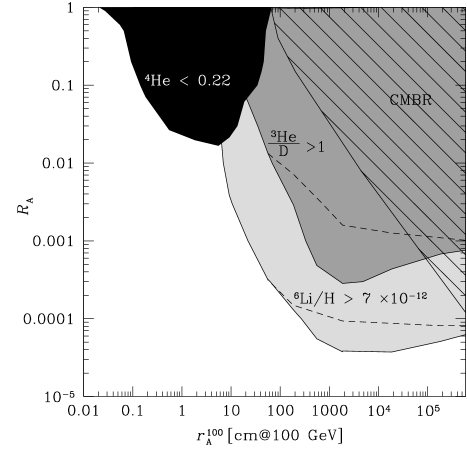
FIG. 10.: Limits on the presence of antimatter in the early Universe. Parameter combinations within the black shaded region result in a ⁴He mass fraction below 0.22, while in the dark grey shaded region the bound ${\rm{{}^{3}\mbox{He}}/^{2}H}<1$ is violated. The excluded range is extended by the light grey shaded region, if one adopts the tentative bound ${\rm{{}^{6}\mbox{Li}}/H}<7\times 10^{-12}$. The dashed lines indicate the results when ⁴He photodisintegration is ignored. Also shown are the usually weaker limits on the presence of antimatter from CMBR considerations (hatched region).

If we employ the new and still slightly speculative ⁶Li limit discussed above, we may significantly tighten the constraints on the amount of antimatter by requiring that pre-galactic production of ⁶Li is not to exceed ${\rm{{}^{6}\mbox{Li}}/H}\lesssim 7\times 10^{-12}$. This leads to an improvement of the limit on ${R_{\rm A}}$ for late time annihilation, i.e. $r_{\rm A}^{100}\gtrsim 6$ cm, by up to two orders of magnitude. This is evident from the light grey shaded region in Fig. 10. Nevertheless, due to the loophole of possible ⁶Li depletion in stars, and due to the still preliminary nature of the ⁶Li observations, this limit should be regarded as tentative at present.

The limits derived from annihilations below $T\lesssim 45$ eV, corresponding to antimatter domain sizes of $r_{\rm A}^{100}\gtrsim 10^{3}\,{\rm cm}$, have to be interpreted with care, since the photodisintegration yields in that regime are uncertain due to the unknown photon spectrum, as we discussed in Sec. IV B. But even if we completely ignore photodisintegration, meaningful limits due to direct production of ³He (and subsequent ⁶Li synthesis) via antiproton annihilation on ⁴He may still be obtained. These limits are indicated by the dashed lines in Fig. 10. Due to the increasing inefficiency of photodisintegration at low temperatures, both limits converge for large antimatter domain sizes.

Note that the limits derived here on the basis of the ³He/²H and ⁶Li data should be similar in magnitude to limits on scenarios where antimatter is homogeneously injected into the plasma, for example by the decay of a relic particle after the nucleosynthesis epoch, since they rely on the production of secondary nuclei from ⁴He disruption and photodisintegration. Both processes are generic for scenarios with injection of antimatter. The competition of annihilation within, and escape from, the annihilation region of the produced light isotopes is, however, particular to a scenario with individual domains. Escape of the annihilation products is inefficient for domain sizes between $\sim 10-100\,$cm, corresponding to the “injection” of antimatter between temperatures $\approx 3-0.4\,$ keV. In this regime more stringent constraints would apply to a homogeneous injection of the antimatter. Furthermore, the reduction of the $n/p$-ratio prior to ⁴He synthesis and thus of the ⁴He mass fraction also only applies to models where antimatter is confined to well defined domains. Only in this case annihilation proceeds via baryon diffusion and thus the differential diffusion of charged and neutral baryons may provide an efficient sink for neutrons. In contrast, a homogeneous injection of antimatter at temperatures above $T_{{}^{4}{\rm He}}\approx 80\,$keV (corresponding approximately to the scale $r_{\rm A}^{100}\approx 6\,$cm in Fig. 10) may be constrained by an increase of $Y_{p}$ due to proton-neutron conversion induced by pion charge exchange [32].

For comparison, we have also shown in Fig. 10 the limits on annihilation which may be derived from the upper limits on distortions of the spectrum of the CMBR. The very precise CMBR data allows us to place constraints on the amount of non thermal energy input at redshifts below $z\approx 3\times 10^{6}$. Each annihilation transforms about one half of the rest mass of the particles into electromagnetically interacting particles, thus the limits given in Ref. [58] may directly be converted into a limit on ${R_{\rm A}}$, which is indicated by the hatched region in Fig. 10. Using the above conservative data set, we find stronger limits from BBN than the ones provided by the CMBR data for annihilations occuring at temperatures above $T_{\rm ann}\gtrsim 1$ eV ($r_{\rm A}^{100}\lesssim 10^{5}$ cm), corresponding to a redshift of $z\gtrsim 4\times 10^{3}$. If we adopt the new ⁶Li bound, the presence of antimatter is more tightly constrained by BBN considerations, rather than by CMBR considerations, for the whole parameter range down to the recombination epoch at $z\approx 10^{3}$.

C Upper Limit on $\Omega_{b}$ in Matter-Antimatter Cosmologies

It is of interest to contemplate if a BBN scenario with matter-antimatter domains may reconcile the observationally inferred element abundances with the theoretically predicted ones for a baryonic density exceeding the upper bound from SBBN, $\Omega_{b}h_{100}^{2}\lesssim 0.02$. Possible alternative solutions to BBN which are in agreement with observationally inferred abundances for higher values of $\Omega_{b}$ have recently received renewed attention due to the results of the Boomerang and MAXIMA experiments [59, 60] on the anisotropies in the CMBR, which favor a baryonic density exceeding the SBBN value [61]. In the standard BBN scenario, such a Universe suffers from overproduction of ⁴He and ⁷Li, and from severe underproduction of ²H. In a scenario with annihilating antimatter domains, there exist two possibilities to reduce the primordial ⁴He mass fraction to the observed value. Early annihilation, prior to ⁴He synthesis, may reduce the $n/p$-ratio and thus the final ⁴He mass fraction. During late time annihilation ⁴He nuclei may be destroyed via antiproton induced disruption and via photodisintegration. At first sight, the possibility to achieve observationally acceptable ⁴He mass fractions at high baryon-to-photon ratios looks promising. But upon closer inspection, some severe shortcomings of such models arise. Scenarios at high net baryon-to-photon ratio and with annihilation prior to ⁴He formation still overproduce ⁷Li relative to the observational constraints. Furthermore, no additional source of ²H exists in this model, which is thus ruled out. In the complementary case, where annihilation is delayed until after the epoch of ⁴He synthesis, production of ²H and ³He due to disruption and photodisintegration of ⁴He results. Even though it is possible to find models where late time ²H production may reproduce the observationally inferred value, the ratio of ³He/²H will exceed unity. This is observationally unacceptable. Further, such a scenario would produce ⁶Li in abundance, which is most likely in conflict with recent observations. This remains true, even if we drop the assumption of a Universe in which the baryon- , or antibaryon-, to-photon ratio has initially the same value throughout the Universe, and furthermore allow the antimatter fraction and domain length scale to take different values at different locations in space. Let us assume that the Universe consists of two different types of regions. In regions of type A with net baryon-to-photon ratio $\eta^{\rm A}_{\rm net}$, the antimatter fraction is high, ${R_{\rm A}}\lesssim 0.25$, and mixing is effective between weak freeze out and ${T_{{}^{4}{\rm He}}}$. Irrespective of the exact value for $\eta^{\rm A}_{\rm net}$, that region consists of protons only after the annihilation is complete. In region B, with net baryon-to-photon ratio $\eta^{\rm B}_{\rm net}$, antimatter domains are larger, so they annihilate after the BBN epoch and light element synthesis may take place. If we further assume that region B is at high baryonic density, $\eta^{\rm B}_{\rm net}\gg\eta_{\rm SBBN}$, the production of ²H and ³He is negligible prior to annihilation. Mass 2 and 3 elements will however be produced in the course of late time annihilation of $\bar{p}$ on ⁴He. It is then easily feasible to find a ratio between the volumes of the two regions such that the average ⁴He mass fraction $\bar{Y}_{\rm p}$ is diluted to the observed value of $Y_{p}\approx 0.25$,

$$\bar{Y}_{\rm p} \approx \frac{\left(Y_{p}\right)_{B}}{1+\frac{\eta^{\rm A}_{\rm net}f_{A}}{\eta^{\rm B}_{\rm net}f_{B}}}\,,$$ (44)

where $f_{A,B}$ are the fractions of space occupied by the two different types of regions, respectively. The ⁴He mass fraction converges to $Y_{p}\approx 0.36$ for high baryonic densities, the required dilution factor is thus at most $(Y_{p})_{B}/Y_{p}\approx 1.5$ in order to obtain $Y_{p}\approx 0.25$. While the ⁴He mass fraction may agree with the observational constraints for an arbitrarily large average baryon density, we face the same problems with production of ²H, ³He and ⁶Li via late time annihilation as discussed above for a one zone model. Furthermore, in region B, ⁷Li is produced well in excess of the observed values and the dilution by mixing with the proton-only zones of type A may not reduce the ⁷Li abundance by more than a factor of 1.5. We thus conclude that it seems difficult to relax the SBBN upper bound on $\Omega_{b}$ by the existence of antimatter domains in the early Universe.

A further result of our study is that the putative presence of antimatter in the early Universe may provide some relieve for the tension between the lower of the two values for the primordial ⁴He mass fraction, $Y_{p}=0.234$ [42], and the low ²H determination, ${}^{2}{\rm H/H}=3.39\times 10^{-5}$ [46]. In view of the recently reported value of $Y_{p}$ derived from observations of the SMC [44], which coincides with the low value, this discrepancy has received new attention. In a Universe at a comparatively high baryon-to-photon ratio of $\eta\approx 5\times 10^{-10}$ with an antimatter fraction of a few $10^{-4}$ distributed on length scales smaller than 6 cm, the abundance yields for ⁴He and ²H may both be ‘low’ and thus the two observational constraints mentioned above may be fulfilled simultaneously.

VII Conclusions

In this work we have studied the mixing and subsequent annihilation of antimatter domains in the early Universe during a period from a cosmological temperature of about 10 MeV, well above the epoch of weak freeze out, down to the formation of neutral hydrogen (recombination) at about 0.2 eV. Such distinct domains of antimatter may possibly arise in some electroweak baryogenesis scenarios [7, 8], as well as in other proposed solutions to the baryogenesis problem (for a review see e.g. [62]). We have shown that the annihilation of antimatter domains may have profound impact on the light element abundances. Depending on the time when annihilation occurs, we identify two main effects. Annihilation prior to the incorporation of all neutrons into ⁴He results mainly in a reduction of the neutron-to-proton ratio, which determines the amount of ⁴He synthesized. Such scenarios are thus constrained by the possible underproduction of ⁴He. Even more stringent constraints on the antimatter-to-matter ratio may be derived if antimatter resides in slightly larger domains and annihilation proceeds after the formation of ⁴He. In this case, the dominant effect is the production of secondary energetic nuclei (²H, ³H, and ³He), which may increase their respective abundances, but may also lead to the production of ⁶Li nuclei. Further, energetic photons originating from the annihilation process may produce additional energetic nuclei via the photodisintegration of ⁴He.

In a second aspect of our work we demonstrated that the presence of small amounts of antimatter, separated from matter within some length scale regime may, in fact, even improve the agreement between BBN theory and observations by reducing the amount of synthesized ⁴He while leaving other light isotope yields basically unaffected. Finally, we argued that the SBBN upper bound on the cosmic baryon density $\Omega_{\rm b}$ is very unlikely to be relaxed in a scenario with annihilating antimatter domains in the early Universe.

A
Structure of the Annihilation Region

In this appendix we will develop a detailed picture about the structure of the annihilation region at the boundaries between matter and antimatter domains. We will also illustrate why the numerical resolution of this thin layer is not essential for making fairly accurate prediction on the light-element nucleosynthesis in an environment with matter-antimatter domains.

In case of annihilation via neutrons, i.e. ${T_{\rm ann}}\gtrsim{T_{{}^{4}{\rm He}}}\approx 80\,{\rm keV}$, diffusion within the annihilation region is — according to the local baryon-to-photon ratio $\eta_{\rm ann}$ — dominated either by magnetic moment scattering on electrons and positrons ($\eta_{\rm ann}\lesssim 10^{-8}$), or by nuclear scattering on protons ($\eta_{\rm ann}\gtrsim 10^{-8}$). In both cases, the typical scattering time for neutrons is much smaller than the annihilation time,

$$\frac{\tau_{ne^{\pm}}}{\tau_{\rm ann}} = \frac{\left(\sigma_{ne}v_{b}n_{e^{\pm}}\right)^{-1}}{\left({\sigma_{\rm ann}v_{b}}n_{\bar{b}}^{\rm ann}\right)^{-1}}$$ (A1)

$$\approx \frac{\left(8\times 10^{-4}\,{\rm mb}\ \sqrt{T/m_{\rm N}}\right)^{-1}}{\Big{(}40\,{\rm mb}\ \eta_{\rm ann}\Big{)}^{-1}}$$ (A2)

$$\approx 6\times 10^{-4}\left(\frac{T}{\,{\rm MeV}}\right)^{-1/2}\left(\frac{\eta_{\rm ann}}{4\times 10^{-10}}\right)$$ (A3)

and

$$\frac{\tau_{np}}{\tau_{\rm ann}} = \frac{\left(\sigma_{np}v_{b}n_{p}\right)^{-1}}{\left({\sigma_{\rm ann}v_{b}}n_{\bar{b}}^{\rm ann}\right)^{-1}}$$ (A4)

$$\approx \frac{\left(2\times 10^{4}\,{\rm mb}\ \sqrt{T/m_{\rm N}}\right)^{-1}}{\Big{(}40\,{\rm mb}\Big{)}^{-1}}$$ (A5)

$$\approx 6\times 10^{-2}\left(\frac{T}{\,{\rm MeV}}\right)^{-1/2}\,.\phantom{\left(\frac{\eta_{\rm ann}}{4\times 10^{-10}}\right)}$$ (A6)

Here $v_{b}$ is a typical baryon thermal velocity, $n_{\bar{b}}^{\rm ann}$ the antibaryon density in the annihilation region, $m_{\rm N}$ the nucleon rest mass and the relevant cross sections are $\sigma_{ne}\approx 8\times 10^{-4}\,{\rm mb}$ and $\sigma_{np}\approx 2\times 10^{4}\,{\rm mb}$ (see e.g. Ref. [20]). Neutron scattering is thus always more probable than annihilation. Note that Eqs. (A3, A6) assume an electron density roughly equal to the photon density, $n_{e^{\pm}}\approx n_{\gamma}$, which is appropriate at early times i. e. before $e^{\pm}$ annihilation, when neutron diffusion is important. In the numerical computations, however, we follow the exact densities of the species.

Annihilation via induced by protons diffusion occurs only in the keV era, where proton diffusion is limited by Thomson scattering of the electrons in the ‘electron-proton system’ off the ambient photons. Even though transport of the protons may now be controlled by hydrodynamic expansion, the movement of the particles over the boundary and inside the annihilation region is still described by diffusion. Comparing the Thomson interaction time with the annihilation time for protons (cf. Eq. 24),

$$\frac{\tau_{e\gamma}}{\tau_{\rm ann}} = \frac{\left(\sigma_{e\gamma}v_{b}n_{\gamma}\right)^{-1}}{\left({\sigma_{\rm ann}v_{b}}n_{\bar{b}}^{\rm ann}\right)^{-1}}$$ (A7)

$$\approx \frac{\left(6.7\times 10^{2}\,{\rm mb}\ \sqrt{T/m_{\rm N}}\right)^{-1}}{\Big{(}32\,{\rm mb}\ \sqrt{\,{\rm MeV}/T}\,\eta_{\rm ann}\Big{)}^{-1}}$$ (A8)

$$\approx 6\times 10^{-7}\left(\frac{T}{\,{\rm keV}}\right)^{-1}\left(\frac{\eta_{\rm ann}}{4\times 10^{-10}}\right),$$ (A9)

we find that the scattering time scale is again much shorter than the annihilation time scale. In both cases, the width of the annihilation region $l^{\rm ann}$ is thus given by the distance $d(\tau_{\rm ann})$ nucleons can diffuse into the respective anti-region during their typical lifetime against annihilation $\tau_{\rm ann}$ (cf. Eq. 11),

$$l^{\rm ann}\approx 2\,d(\tau_{\rm ann})\approx 2\,\left(\int_{0}^{\tau_{\rm ann}}6D(t){\rm d}t\right)^{1/2}\approx 2\sqrt{6D\tau_{\rm ann}}\;.$$ (A10)

We have included a factor of 2 to allow for diffusion of matter into the antimatter region as well as of antimatter into the matter region. The diffusion constant $D$ can be taken to be constant over the lifetime against annihilation. In order to calculate $\tau_{\rm ann}$, we need to estimate the density in the annihilation region. We assume that a steady state between diffusion of baryon number into the annihilation region and annihilation of this baryon number is established. The concept of a steady state is only appropriate for times somewhat shorter than the Hubble time, since the densities and diffusion constants vary with the expansion of the Universe. A typical baryonic density gradient some distance away from the annihilation region will however always be of the order of $\Delta n_{b}/d_{b}(\tau_{\rm Hubble})$, with $d_{b}(\tau_{\rm Hubble})$ the diffusion length scale over one Hubble time. The difference in baryon density is given by $\Delta n_{b}=\tilde{n}_{b}-n_{b}^{\rm ann}$, with $\tilde{n}_{b}$ the baryon density far away from the annihilation region and $n_{b}^{\rm ann}$ the baryon density within the annihilation region. The baryon density in the annihilation region will typically be much smaller than $\tilde{n}_{b}$; therefore we replace $\Delta n_{b}$ by $\tilde{n}_{b}$. This leads us to approximate the baryon number flux $F_{b}$ into the annihilation region by

$$F_{b} = D\nabla n_{b}A\approx D\frac{\Delta n_{b}}{d_{b}(\tau_{\rm Hubble})}A\approx D\frac{\tilde{n}_{b}}{d_{b}(\tau_{\rm Hubble})}A\;.$$ (A11)

The number of annihilations in a volume with surface $A$ and width $l^{\rm ann}$ should then be equal to the flux of baryons into the volume,

$${\sigma_{\rm ann}v_{b}}n_{b}^{\rm ann}n_{\bar{b}}^{\rm ann}\,A\,l^{\rm ann} = D\frac{\tilde{n}_{b}}{d_{b}(\tau_{\rm Hubble})}A\;.$$ (A12)

As long as the diffusion length is considerably smaller than the size of the antimatter region, $\tilde{n}_{b}$ is equal to the initial matter density, $\tilde{n}_{b}=\bar{n}^{\rm net}\Delta^{0}$, where $\Delta^{0}$ is the initial baryon overdensity and $\bar{n}^{\rm net}$ the initial average net baryon density (see Eq. 1). We may now compute the baryon density in the annihilation region. Inserting the annihilation length $l^{\rm ann}$, Eq. (A10), into Eq. (A12) and using $\tau_{\rm ann}=({\sigma_{\rm ann}v_{b}}n_{\bar{b}}^{\rm ann})^{-1}$ yields

$${\sigma_{\rm ann}v_{b}}n_{b}^{\rm ann}n_{\bar{b}}^{\rm ann}2A\sqrt{\frac{6\,D}{{\sigma_{\rm ann}v_{b}}n_{\bar{b}}^{\rm ann}}} = D\frac{\bar{n}^{\rm net}\Delta^{0}}{\sqrt{D\,\tau_{\rm Hubble}}}A\;.$$ (A13)

The baryon and antibaryon density within the annihilation region should be of the same magnitude, thus we finally obtain for the baryon density in the annihilation region

$$n_{b}^{\rm ann} = \left(\frac{(\bar{n}^{\rm net}\Delta^{0})^{2}}{6{\sigma_{\rm ann}v_{b}}\tau_{\rm Hubble}}\right)^{1/3}.$$ (A14)

This may be written in terms of the local baryon overdensity $\Delta^{\rm ann}$ in the annihilation region as

$$\Delta^{\rm ann} \equiv \frac{n_{b}^{\rm ann}}{\bar{n}^{\rm net}}$$ (A15)

$$= 2.4\times 10^{-3}\,(\Delta^{0})^{2/3}\left(\frac{{\sigma_{\rm ann}v_{b}}}{40\,\,{\rm mb}\,c}\right)^{-1/3}$$ (A17)

$$\times\left(\frac{\,{\rm MeV}}{T}\right)^{1/3}\left(\frac{\eta}{4\times 10^{-10}}\right).$$

Interestingly, the overdensity in the annihilation region $\Delta^{\rm ann}$ is independent of the diffusion constant. We may now calculate the width of the annihilation region in our comoving units,

$$l^{\rm ann}_{100} = \frac{2}{R}\,\left(\frac{6\,D}{{\sigma_{\rm ann}v_{b}}\,\bar{n}^{\rm net}\Delta^{\rm ann}}\right)^{1/2}.$$ (A18)

Using the relevant diffusion constants and annihilation cross sections and further assuming $\eta_{\rm net}=4\times 10^{-10}$, we obtain

$$l^{\rm ann}_{100} = 2\times 10^{-4}\,{\rm cm}\,(\Delta^{0})^{-1/3}\left(\frac{T}{\,{\rm MeV}}\right)^{-19/12}$$ (A19)

for annihilation via neutron diffusion and

$$l^{\rm ann}_{100} = 1.3\times 10^{-1}\,{\rm cm}\,(\Delta^{0})^{-1/3}\left(\frac{T}{\,{\rm keV}}\right)^{-17/12}$$ (A20)

for annihilation via proton diffusion.

FIG. 11.: Left panel: Snapshot of the neutron (full line) and the antineutron (dotted line) overdensity, $\Delta_{\rm n}$ and $\Delta_{\bar{n}}$ at a temperature of $T\approx 10\,{\rm MeV}$. This distribution was obtained with a high resolution simulation; the antimatter parameters were ${R_{\rm A}}$ = 0.9 and $r_{\rm A}^{100}$ = $1.5\times 10^{-2}\,{\rm cm}$. Right panel: Zoom into the annihilation region. See text for discussion.

We have numerically verified Eq. (A19) for a scenario with antimatter regions of size $r_{\rm A}^{100}=1.5\times 10^{-2}\,{\rm cm}$ and an initial overdensity $\Delta^{0}\approx 10$, corresponding to a matter-antimatter ratio of ${R_{\rm A}}=0.9$. In order to check the validity of the assumption of a steady state, we had to let the code evolve at least over the period of one Hubble time. The two snapshots of the neutron and antineutron overdensity, $\Delta_{n}$ and $\Delta_{\bar{n}}$ (cf. Fig. 11) were obtained in a simulation which was started at $T\approx 20\,{\rm MeV}$, and evolved down to $T\approx 10\,{\rm MeV}$. The left panel shows the whole simulation volume, while the right panel is a zoom into the annihilation region of the same simulation. The resolution is fine enough to describe (anti-)neutron diffusion within the annihilation region. We find an overdensity in the central region of $\Delta^{\rm ann}\approx\mbox{\it a\ few}\,10^{-3}$ which may be compared to the above estimate, $\Delta^{\rm ann}\approx 3\times 10^{-3}$. The width of the annihilation region is $l^{\rm ann}_{100}\approx 10^{-6}\,{\rm cm}$, following Eq. (A19).

Since the two relevant processes — transport of particles through their own region towards the annihilation region and diffusion within the anti-region — proceed on length scales which differ by orders of magnitude, it is very time-consuming to run simulations with the resolution necessary to adequately describe both processes. The numerical results presented in this work were obtained at a resolution which properly resolves the transport processes over the distance of order of the domain size, but does not resolve the diffusion within the annihilation region. This should however affect our results little, since the exact composition of the annihilation region is not decisive for the final abundances.

In case of annihilation before ⁴He synthesis, the exact annihilation time is crucial for our results. Protons hardly play a role in case of early annihilation due to their very short diffusion length. The protons which are originally present in the annihilation region are quickly annihilated. Additional protons may not be transported into the annihilation region and their density profile remains frozen in. The annihilation region is thus populated by neutrons and antineutrons only, and further annihilation may only proceed via neutrons and antineutrons. All particles which reach the annihilation region will inevitably be annihilated on a very short time scale compared to the transport time. Thus the time scale for annihilation of all antimatter is set by the transport of neutrons and antineutrons towards the annihilation region, hence over considerably longer distances than the annihilation region, which are properly resolved.

In case of annihilation after the disappearance of free neutrons at a temperature of ${T_{{}^{4}{\rm He}}}\approx 80\,{\rm keV}$, the dominant channels are $\bar{p}$$p$ and $\bar{p}$⁴He. The ratio of annihilations on either ⁴He or on protons is important, since this ratio determines how many secondary nuclei, which arise in ⁴He disruption, are produced for a given antimatter fraction. This ratio depends again on the transport of the nuclei over the whole matter region into the annihilation region. The transport time scale may either be set by charged particle diffusion or by hydrodynamic expansion. For both processes, resolution of the whole simulation volume is important, but since again all nuclei which reach the annihilation region are inevitably annihilated, the spatial distribution of the nuclei within the annihilation region should be of negligible importance.

The effect of not resolving the annihilation region is that matter and antimatter may travel further into the respective anti-region than is physically correct. But since in both cases discussed above the number of annihilations on a specific nucleus at a specific time is set by the transport processes, this lack of resolution should not be relevant. The relative independence of the results on the exact structure of the annihilation region is also evident by resolution studies given in App. B.

Energetic secondary nuclei arising in the ⁴He disruption process may only escape from the annihilation region and thus influence the final abundance yields if their stopping length is much larger than the annihilation region. The correct treatment of this effect is therefore independent of whether or not diffusion within the annihilation region is resolved.

B Numerical Methods

The task of performing detailed numerical BBN calculations was first fulfilled by Wagoner, Fowler & Hoyle [18]. Jedamzik & Fuller [20, 41] developed an inhomogeneous BBN code to describe the evolution of subhorizon-scale baryon-to-photon fluctuations in the early Universe and the resultant modifications of the light element abundances. To this end, a Lagrangian grid of zones was introduced in which the various thermodynamic quantities and the nuclear densities may deviate from the respective horizon average value. The BBN network is coupled to all relevant hydrodynamic processes, such as diffusion of baryons, photon diffusive heat transport, neutrino heat transport and late-time hydrodynamic expansion of high-density regions. The nuclear reaction network and the thermodynamic evolution of the homogeneous radiation background is treated as in an updated version of the original BBN code [63, 19]. Baryon diffusion and incorporation of baryons into nuclei proceeds on fast time scales, it is thus necessary to treat baryon diffusion implicitly. Further, neutrino and photon heat transport and hydrodynamic processes are included in the code.

FIG. 12.: Light element abundances obtained in simulations with three different combinations of the antimatter parameters (see legend). The number of zones was varied between 20 and 70 to check for convergence of the results.

We extended the inhomogeneous code [20, 41] to include antielements and adapted it to the present problem. We use a set of concentric spherical shells to describe the distribution of matter and antimatter. The number of zones in the simulations has to be chosen such, that the spatial resolution of the volume is sufficient to adequately describe the relevant physical processes. It turned out that 30 zones are sufficient to resolve diffusion of the nuclei and obtain reasonable convergence in the final abundances (see Fig. 12). The region where most of the annihilations occur, on the other hand, has not been resolved in our simulations. The results should however be fairly insensitive to the actual structure of the thin annihilation layer, as we discuss in App. A.

The whole procedure of solving the nuclear reaction matrix and the treatment of the hydrodynamical processes is included in a second order Runge-Kutta scheme, i.e. it has to be done twice per time step. The results of the two Runge-Kutta steps are averaged at the end of each time step. Since not only the densities within each zone, but also the radii of the zones may change, this has to be done very carefully in order to minimize errors. An adequate independent check of the numerical simulations is the achieved accuracy in baryon number conservation. Generally, the baryon number is conserved on the level of $\Delta N_{b}/N_{b}\lesssim{\cal O}(10^{-6})$ for those regions of the parameter space relevant for the derivation of our limits. Only for large antimatter fractions, ${R_{\rm A}}\gtrsim 0.5$ on length scales $r_{\rm A}^{100}\gtrsim 10\,{\rm cm}$, numerical conservation of baryon number deteriorates. It seems however very unlikely to find an observationally acceptable scenario for combinations of the parameters in that range such that the simulation of such scenarios is of little interest.

The escape of ⁶Li and the mass three nuclei from the annihilation region was treated as follows. We keep track of the number of ³H, ³He and ⁶Li nuclei produced in $\bar{p}$⁴He annihilations during a single time step. Using the stopping length for these nuclei according to Eq. (28) we may calculate the fraction of those thermalized within the matter region by geometrical considerations. This fraction is then added to the number density of the respective nuclei.

REFERENCES

- [1] G. Steigman, Ann. Rev. Astron. Astroph. 14, 339 (1976).
- [2] A. Cohen, A. de Rújula, and S. Glashow, ApJ495, 539 (1998).
- [3] W. H. Kinney, E. W. Kolb, and M. S. Turner, Phys. Rev. Lett.79, 2620 (1997).
- [4] A. G. Cohen and A. de Rújula, ApJ496, L63 (1998).
- [5] A. Dolgov and J. Silk, Phys. Rev. D47, 4244 (1993).
- [6] R. A. Sunyaev and Ya. B. Zel’dovich, Astrophys. Sp. Science 7, 20 (1970).
- [7] D. Comelli, M. Pietroni, and A. Riotto, Nuc. Phys. B412, 441 (1994).
- [8] M. Giovannini and M. E. Shaposhnikov, Phys. Rev. Lett.80, 22 (1998). M. Giovannini and M. E. Shaposhnikov, Phys. Rev. D57, 2186 (1998).
- [9] M. Yu. Khlopov, S. G. Rubin, and A. S. Sakharov, hep-ph/0003285 (2000).
- [10] J. B. Rehm and K. Jedamzik, Phys. Rev. Lett.81, 3307 (1998).
- [11] H. Kurki-Suonio and E. Sihvola, Phys. Rev. Lett.84, 3756 (2000).
- [12] G. Steigman, Cal-Tech Orange Aid OAP 280, (1972); F. Combes, O. Fassi-Fehri, and B. Leroy, Astrophys. Sp. Science 37, 151 (1975); J. J. Aly, Astron. Astrophys.64, 273 (1978).
- [13] V. M. Chechetkin, M. Yu. Khlopov, M. G. Sapozhnikov, and Ya. B. Zel’dovich, Phys. Lett. B118, 329 (1982); V. M. Chechetkin, M. Yu. Khlopov, and M. G. Sapozhnikov, Riv. Nuovo Cim. 5, 1 (1982).
- [14] Yu. A. Batusov et al., Nuovo Cim. Lett. 41, 223 (1984).
- [15] M. Yu. Khlopov and A. D. Linde, Phys. Lett. B138, 265 (1984); J. Ellis, D. V. Nanopoulos, and S. Sarkar, Nuc. Phys. B259, 175 (1985); D. Lindley, Phys. Lett. B171, 235 (1986); R. Domínguez-Tenreiro, ApJ313, 523 (1987); I. Halm, Phys. Lett. B188, 403 (1987).
- [16] R. Domínguez-Tenreiro and G. Yepes, ApJ317, L1 (1987); G. Yepes and R. Domínguez-Tenreiro, ApJ335, 3 (1988).
- [17] Yu. B. Zel’dovich, A. A. Starobinskii, M. Yu. Khlopov, and V. M. Chechetkin, Pis’ma Astron. Zh. 3, 208 (1977); B. V. Vainer, O. V. Dryzhakova, and P. D. Naselskii, Pis’ma Astron. Zh. 4, 344 (1978).
- [18] R. V. Wagoner, W. A. Fowler, and F. Hoyle, ApJ148, 3 (1967).
- [19] M. S. Smith, L. H. Kawano, and R. A. Malaney, ApJ Suppl. Ser. 85, 219 (1993).
- [20] K. Jedamzik and G. Fuller, ApJ423, 33 (1994).
- [21] J. H. Applegate, C. J. Hogan, and R. J. Scherrer, Phys. Rev. D35, 1151 (1987).
- [22] Here we have corrected for an obvious mistake in Ref. [20].
- [23] C. R. Alcock, D. S. Dearborn, G. M. Fuller, G. J. Mathews, and B. S. Meyer, Phys. Rev. Lett.64, 2607 (1990).
- [24] P. J. E. Peebles, Physical Cosmology (Princeton University Press, Princeton, NJ, 1971).
- [25] F. Balestra, S. Bossolasco, M. P. Bussa, L. Busso, and L. Fava, Nuovo Cim. 100A, 323 (1988).
- [26] J. Carbonell, K. V. Protasov, and A. Zenoni, Phys. Lett. B397, 345 (1997).
- [27] K. V. Protasov, G. Bonomi, E. L. Rizzini, and A. Zenoni, Eur. Phys. J. A7, 429 (2000).
- [28] A. Zenoni et al., Phys. Lett. B461, 413 (1999); A. Zenoni et al., Phys. Lett. B461, 405 (1999).
- [29] G. S. Mutchler et al., Phys. Rev. D38, 742 (1988).
- [30] J. Carbonell and K. Protasov, Hyperfine Interactions 76, 327 (1993).
- [31] J. Carbonell and K. V. Protasov, Z. Phys. A 355, 87 (1996).
- [32] M. H. Reno and D. Seckel, Phys. Rev. D37, 3441 (1988).
- [33] D. Lindley, Mon. Not. Roy. Astron. Soc. 193, 593 (1980).
- [34] J. Ellis, G. Gelmini, J. Lopez, D. Nanopoulos, and S. Sarkar, Nuc. Phys. B373, 399 (1992).
- [35] R. Protheroe, T. Stanev, and V. Berezinsky, Phys. Rev. D51, 4134 (1995).
- [36] K. Jedamzik, Phys. Rev. Lett.84, 3248 (2000).
- [37] J. D. Jackson, Classical Electrodynamics (John Wiley & Sons, New York, 1975).
- [38] S. Dimopoulos, R. Esmailzadeh, L. Hall, and G. Starkmann, ApJ330, 545 (1988).
- [39] The production of 7Li via T + 4He 7Li is less efficient due to a smaller cross section of mb.
- [40] J. P. Meyer, Astron. Astrophys. Suppl. 7, 417 (1972).
- [41] K. Jedamzik, G. M. Fuller, and G. J. Mathews, ApJ423, 50 (1994).
- [42] K. A. Olive, E. Skillman, and G. Steigman, ApJ483, 788 (1997).
- [43] Y. I. Izotov and T. X. Thuan, ApJ500, 188 (1998).
- [44] M. Peimbert, A. Peimbert, and M. T. Ruiz, astro-ph/0003154 (2000).
- [45] J. K. Webb et al., Nature388, 250 (1997).
- [46] S. Burles and D. Tytler, ApJ507, 732 (1998).
- [47] S. A. Levshakov, W. H. Kegel, and F. Takahara, ApJ499, L1 (1998).
- [48] G. Sigl, K. Jedamzik, D. N. Schramm, and V. S. Berezinsky, Phys. Rev. D52, 6682 (1995).
- [49] J. Geiss, in Origin and Evolution of the Elements, edited by N. Prantzos, E. Vangioni-Flam, and M. Cassé (Cambridge University Press, Cambridge, UK, 1993).
- [50] V. V. Smith, D. L. Lambert, and P. E. Nissen, ApJ408, 262 (1993); L. M. Hobbs and J. A. Thorburn, ApJ428, L25 (1994); R. Cayrel, M. Spite, F. Spite, E. Vangioni-Flam, M. Cassé, and J. Audouze, Astron. Astrophys.343, 923 (1999).
- [51] P. E. Nissen, D. L. Lambert, F. Primas, and V. V. Smith, Astron. Astrophys.348, 211 (1999).
- [52] P. Bonifacio and P. Molaro, Mon. Not. Roy. Astron. Soc. 285, 847 (1997).
- [53] M. H. Pinsonneault, C. P. Deliyannis, and P. Demarque, ApJ Suppl. Ser. 78, 179 (1992).
- [54] B. Chaboyer and P. Demarque, ApJ433, 510 (1994).
- [55] S. G. Ryan, J. E. Norris, and T. C. Beers, ApJ523, 654 (1999).
- [56] S. G. Ryan, T. C. Beers, K. A. Olive, B. D. Fields, and J. E. Norris, ApJ530, L57 (2000).
- [57] We note here that adopting the more conservative constraint , for example, would hardly change the constraints on shown in Fig. 10.
- [58] D. J. Fixsen et al., ApJ473, 576 (1996).
- [59] P. de Bernardis et al., Nature404, 955 (2000).
- [60] A. Balbi et al., astro-ph/0005124 (2000).
- [61] A. E. Lange et al., astro-ph/0005004 (2000); J. Lesgourgues and M. Peloso, astro-ph/0004412 (2000); M. Tegmark and M. Zaldarriaga, astro-ph/0004393 (2000); S. Hanany et al., astro-ph/0005123 (2000).
- [62] A. D. Dolgov, in Proceedings of International Workshop on Future Prospects of Baryon Instability Search in p-Decay and Oscillation Experiments, Oak Ridge, TN, USA ; 28 - 30 Mar 1996, edited by S. J. Ball and Y. A. Kamyshkov (National Laboratory, Oak Ridge, TN, 1996), p. 101.
- [63] L. Kawano, FERMILAB-Pub-92/04-A (1992).