Resolving the Structure of Cold Dark Matter Halos

Abstract

We present results of a convergence study in which we compare the density profiles of CDM dark matter halos simulated with varying mass and force resolution. We show that although increasing the mass and force resolution allows one to probe deeper into the inner halo regions, the halo profiles converge at scales larger than the “effective” spatial resolution of the simulation. This resolution is defined both by the force softening and by the mass resolution. On radii larger than the “effective” spatial resolution, density profiles do not experience any systematical trends when the number of particles or the force resolution increase further. In the simulations presented in this paper, we are able to probe density profile of a relaxed isolated galaxy-size halo at scales $r=(0.005-1)\mbox{$r_{\rm vir}$}$. We find that the density distribution at resolved scales can be well approximated by the profile suggested by Moore et al.(1998): $\rho\propto x^{-1.5}(1+x^{1.5})^{-1}$, where $x=r/\mbox{$r_{\rm s}$}$ and $r_{\rm s}$  is the characteristic radius. The analytical profile proposed by Navarro et al. (1996) $\rho\propto x^{-1}(1+x)^{-2}$, also provides a good fit, with the same relative errors of about 10% for radii larger than 1% of the virial radius. For this limit both analytical profiles fit well because for high-concentration galaxy-size halos the differences between these profiles become significant only at scales well below $0.01\mbox{$r_{\rm vir}$}$. We also find that halos of similar mass may have somewhat different parameters (characteristic radius, maximum rotation velocity, etc.) and shapes of their density profiles. We associate this scatter in properties with differences in halo merger histories and the amount of substructure present in the analyzed halos.

1 Introduction

During the last decade there has been an increasingly growing interest in testing the predictions of variants of cold dark matter (CDM) models at subgalactic ($\lesssim 100{\rm\ kpc}$) scales. This interest was initiated by indications that observed rotation curves in the central regions of dark matter dominated dwarf galaxies are at odds with predictions of hierarchical models. Specifically, it was argued (Flores & Primack 1994; Moore 1994) that circular velocities, $v_{c}(r)\equiv[GM(<r)/r]^{1/2}$, at small galactocentric radii predicted by the models are too high and increase too rapidly with increasing radius compared to the observed rotation curves. The steeper than expected rise of $v_{c}(r)$ implies that the shape of the predicted halo density distribution is incorrect and/or that the DM halos formed in CDM models are too concentrated (i.e., have too much of their mass concentrated in the inner regions).

In addition to the density profiles, there is an alarming mismatch in the predicted abundance of small-mass ($\lesssim 10^{8}-10^{9}\mbox{$h^{-1}$M${}_{\odot}$}$) galactic satellites and the observed number of satellites in the Local Group (Kauffmann, White & Guiderdoni 1993; Klypin et al. 1999; Moore et al. 1999). Although this discrepancy may well be due to feedback processes (such as photoionization) which prevent gas collapse and star formation in the majority of the small-mass satellites (e.g., Bullock, Kravtsov & Weinberg 2000), the mass scale at which the problem sets in is similar to the scale in the spectrum of primordial fluctuations that may be responsible for the problems with density profiles. In the age of precision cosmology that forthcoming MAP and Planck cosmic microwave background anisotropy satellite missions are expected to bring, tests of the cosmological models at small scales may prove to be the final frontier and the ultimate challenge to our understanding of cosmology and structure formation in the Universe. However, this obviously requires detailed predictions and checks from the theoretical side, as well as higher resolution/quality observations and a good understanding of their implications and associated caveats. In this paper we focus on the theoretical predictions of the density distribution of DM halos.

A systematic study of halo density profiles for a wide range of halo masses and cosmologies was done by Navarro, Frenk & White (1996, 1997; hereafter NFW), who argued that the analytical profile of the form $\rho(r)=\rho_{s}(r/r_{s})^{-1}(1+r/r_{s})^{-2}$ provided a good description of halo profiles in their simulations for all halo masses and in all cosmologies. Here, $r_{s}$ is the scale radius which, for this profile, corresponds to the scale at which $d\log\rho(r)/d\log r|_{r=r_{s}}=-2$. The parameters of the profile are determined by the halo’s virial mass $M_{\rm vir}$ and concentration defined as $c\equiv\mbox{$r_{\rm vir}$}/r_{s}$. NFW argued that there is a tight correlation between $c$ and $M_{\rm vir}$, which implies that the density distributions of halos of different masses can in fact be described by a one-parameter family of analytical profiles. Further studies by Kravtsov, Klypin & Khokhlov (1997), Kravtsov et al. (1998, hereafter KKBP98), Jing (2000), Bullock et al. (2000), although confirming the $c(\mbox{$M_{\rm vir}$})$ correlation, indicated that there is significant scatter in both the density profiles and concentrations for DM halos of a given mass.

Following the initial studies by Flores & Primack (1994) and Moore (1994), KKBP98 presented a systematic comparison of the results of numerical simulations with rotation curves of a sample of seventeen dark matter dominated dwarf and low surface brightness (LSB) galaxies.

We pointed out that the measured rotation curves of these galaxies all had the same shape with nearly linear central behavior, and furthermore, based on comparison with the density profiles of simulated halos there did not seem to be a significant discrepancy in the shape of the density profiles at the scales probed by the numerical simulations ($\gtrsim 0.02-0.03\mbox{$r_{\rm vir}$}$, where $r_{\rm vir}$ is halo’s virial radius). In other words, the central density distribution in both galaxies and CDM halos was found to be shallower than $\propto r^{-1}$. These conclusions were subject to several caveats and required further testing. First, observed galactic rotation curves had to be re-examined more carefully and with higher resolution. The fact that all of the observed rotation curves used in earlier analyses were obtained using relatively low resolution HI observations required checks of the possible beam smearing effects. Also, the possibility of non-circular random motions in the central regions which could modify the rotation velocity of the gas (e.g., Binney & Tremain 1987, p. 198) had to be considered. Second, the theoretical predictions had to be tested for convergence and extended to scales $\lesssim 0.01\mbox{$r_{\rm vir}$}$.

Moore et al. (1998; see also a more recent convergence study by Ghigna et al. 1999) presented a convergence study arguing that mass resolution has a significant impact on the central density distribution of halos. They suggested that at least several million particles per halo are required to reliably model the density profiles at scales $\lesssim 0.01\mbox{$r_{\rm vir}$}$. Based on these results, Moore et al. (1998) advocated a density profile of the form $\rho(r)\propto(r/r_{s})^{-1.5}[1+(r/r_{s})^{1.5}]^{-1}$, that behaves similarly ($\rho\propto r^{-3}$) to the NFW profile at large radii, but is steeper at small $r$: $\rho\propto r^{-1.5}$. Most recently, Jing & Suto (2000) presented a systematic study of density profiles for halo masses in the range $2\times 10^{12}\mbox{$h^{-1}$M${}_{\odot}$}-5\times 10^{14}\mbox{$h^{-1}$M${}_{\odot}$}$. The study was uniform in mass and force resolution featuring $\sim 5-10\times 10^{5}$ particles per halo and force resolution of $\approx 0.004\mbox{$r_{\rm vir}$}$. They found that galaxy-mass halos in their simulations are well fitted by the profile $\rho(r)\propto(r/r_{s})^{-1.5}[1+r/r_{s}]^{-1.5}$, but that cluster-mass halos are well described by the NFW profile, with logarithmic slope of the density profiles at $r=0.01\mbox{$r_{\rm vir}$}$ changing from $\approx-1.5$ for $\mbox{$M_{\rm vir}$}\sim 10^{12}\mbox{$h^{-1}$M${}_{\odot}$}$ to $\approx-1.1$ for $\mbox{$M_{\rm vir}$}\sim 5\times 10^{14}\mbox{$h^{-1}$M${}_{\odot}$}$. Jing & Suto interpreted these results as an evidence that profiles of DM halos are not universal (but see §3.1 for a possible alternative interpretation).

At small scales, the results of Kravtsov et al. (1998) are at odds with the results of above studies. Although fairly extensive convergence tests were done in that study, they focused on the effects of spatial resolution and the mass resolution was kept constant in almost all the tests. In this case we found that halo density profiles converged at scales larger than two formal resolutions of the ART code. As we will show in this paper, this is not true when the mass resolution is varied. In particular, the convergence study presented in this paper in which we varied both mass and force resolution shows that for the ART simulations convergence is reached at scales larger than four formal resolutions or the scales containing 200 particles, whichever is larger. The shallow behavior of the density profiles in Kravtsov et al. was found at scales $\approx 2-5$ formal resolutions (at larger scales profiles were consistent with the NFW functional form) and is therefore a numerical artifact. In simulations presented in this paper we find profiles that are consistent with cuspy NFW and Moore et al. distributions at well resolved scales.

New observational and theoretical developments show that comparison between model predictions and observational data is not straightforward. Decisive comparisons require reaching convergence of theoretical predictions and understanding the kinematics of the gas in the central regions of observed galaxies. As we noted above, in this paper we present convergence tests designed to test effects of mass resolution on the density profiles of halos formed in the currently popular CDM model with cosmological constant ($\Lambda$CDM) and simulated using the multiple mass resolution version of the Adaptive Refinement Tree code (ART). This study is crucial in resolving the discrepancy of our previous study on the density profiles with other numerical studies. We also discuss several caveats with respect to drawing conclusions about the density profiles from the fits of analytical functions to numerical results and their comparisons to observational data. In the following section we describe the code and numerical simulations used in our analysis. In §3 we compare the analytical fits advocated by NFW and Moore et al., fits of these profiles to the density profiles of simulated halos, and convergence analysis of our numerical results.

2 Numerical simulations

2.1 Code description

The Adaptive Refinement Tree code (ART; Kravtsov, Klypin & Khokhlov 1997) was used to run the simulations. The ART code starts with a uniform grid, which covers the whole computational box. This grid defines the lowest (zeroth) level of resolution of the simulation. The standard Particles-Mesh algorithms are used to compute density and gravitational potential on the zeroth-level mesh. The ART code reaches high force resolution by refining all high density regions using an automated refinement algorithm. The refinements are recursive: the refined regions can also be refined, each subsequent refinement having half of the previous level’s cell size. This creates a hierarchy of refinement meshes of different resolution, size, and geometry covering regions of interest. Because each individual cubic cell can be refined, the shape of the refinement mesh can be arbitrary and match effectively the geometry of the region of interest.

The criterion for refinement is the local density of particles: if the number of particles in a mesh cell (as estimated by the Cloud-In-Cell method) exceeds the level $n_{\rm thresh}$, the cell is split (“refined”) into 8 cells of the next refinement level. The refinement threshold may depend on the refinement level. The code uses the expansion parameter $a$ as the time variable. During the integration, spatial refinement is accompanied by temporal refinement. Namely, each level of refinement, $l$, is integrated with its own time step $\Delta a_{l}=\Delta a_{0}/2^{l}$, where $\Delta a_{0}$ is the global time step of the zeroth refinement level. This variable time stepping is very important for accuracy of the results. As the force resolution increases, more steps are needed to integrate the trajectories accurately. In the remainder of the paper by the term formal resolution, $h_{\rm formal}$, we will mean the size of a cell on the highest level of refinement reached in simulation. This is similar to the usual practice of defining formal resolution in the uniform grid codes. The actual force resolution of the code is somewhat larger than the formal resolution. In the ART code, the interparticle force is weaker (“softer”) than the Newtonian force at scales $<2h_{\rm formal}$. The average interparticle force is Newtonian at scales $\mathrel{\mathchoice{\lower 0.5pt\vbox{\halign{$\mathnew\displaystyle\hfil#\hfil$\cr>\crcr\sim\crcr}}}{\lower 0.5pt\vbox{\halign{$\mathnew\textstyle\hfil#\hfil$\cr>\crcr\sim\crcr}}}{\lower 0.5pt\vbox{\halign{$\mathnew\scriptstyle\hfil#\hfil$\cr>\crcr\sim\crcr}}}{\lower 0.5pt\vbox{\halign{$\mathnew\scriptscriptstyle\hfil#\hfil$\cr>\crcr\sim\crcr}}}}2h_{\rm formal}$, although there is a substantial scatter in the force at $\approx 2-3h_{\rm formal}$ due primarily to errors in numerical differentiation of potential. For comparison, average Plummer softened force with softening $\epsilon_{\rm Plummer}=h_{\rm formal}$, reaches the Newtonian value at scales $\approx 5-6h_{\rm formal}$ (see Kravtsov et al. 1997 for details). Therefore, one formal resolution in the ART code is equivalent to $\approx 0.3-0.4$ Plummer softening of the same value.

The cosmological simulations performed using the ART code were compared with the simulations started from identical initial conditions and performed using the well-known PM and AP³M codes. The comparisons showed that results of ART simulations (for a wide battery of the commonly used statistics and halo parameters) are similar to those of the AP³M simulations at all resolved scales. These comparisons and other tests of the ART code can be found in Kravtsov (1999) and Knebe et al. (2000).

2.2 Initial conditions

The current version of the ART code has the ability to handle particles of different masses. In the present analysis this ability was used to increase the mass (and correspondingly the force) resolution inside a few pre-selected halos. The multiple mass resolution is implemented in the following way. We set up a realization of the initial spectrum of perturbations in such a way that a very large number of small-mass particles can be generated in the simulation box. For example, for the first (second) set of simulations (see below) we generate $512^{3}$ ($1024^{3}$) independent spectrum harmonics. Potentially, initial conditions with $512^{3}/1024^{3}$ particles could be generated. Coordinates and velocities of the particles are calculated using all waves ranging from the fundamental mode $k=2\pi/L$ to the Nyquist frequency $k=2\pi/L\times N^{1/3}/2$, where $L$ is the box size and $N$ is the number of particles in the simulation.

The code actually generates positions and velocities for all $512^{3}/1024^{3}$ particles, but some of the particles are then merged into particles of larger mass. The larger mass (merged) particle is assigned velocity and displacement equal to the average velocity and displacement of the merged particles. The whole lagrangian space of particles is divided into large cubic blocks of particles with each block having $16^{3}$ particles. Depending on what local mass resolution is required, each particular block can be subdivided into smaller sub-blocks and generate from 1 to $16^{3}$ particles (the highest resolution). Using this procedure, we can generate particles with 5 different masses covering dynamic mass range of 4096.

We start simulations by making a low resolution run with uniform mass resolution in which all particles have the largest possible mass. Next we run simulations with $32^{3}$ and $64^{3}$ particles. Using these runs, we identify halos in the simulation and select halos to be re-simulated with higher mass and force resolution. For each selected halo we determine its virial radius. We then identify all particles inside the two virial radii and find lagrangian coordinates of each particle. The coordinates are used to mark blocks of particles to generate the initial conditions of the highest mass resolution. Once all particles are processed and all blocks are marked, we mark all blocks adjacent to those already marked to produce initial conditions of the eight times lower mass resolution. This procedure is repeated for lower and lower mass resolution levels. In the end, each unmarked block will produce one most massive particle and a marked block will generate a number of particles which depends on the step in which the block was marked. Figure 1 shows the outcome of the process of mass refinement in a 2-dimensional case.

Figure 2 shows an example of mass refinement for one of the halos in our simulations. A large fraction of high resolution particles ends up in the central halo, which does not have any larger mass particles (see insert in the bottom panel). At $z=10$, the region occupied by the high resolution particles is non-spherical: it is substantially elongated in the direction perpendicular to the large filament clearly seen at $z=0$.

Figure 1: Example of the construction of mass refinement in lagrangian space (here for illustration we show a 2D case). Three central blocks of particles were marked for highest mass resolution. Each block produces $16^{2}$ particles of the smallest mass. Adjacent blocks correspond to the four times lower resolution and produce $8^{2}$ particles each. The procedure is repeated recursively until we reach the lowest level of resolution. The region of the highest resolution can have arbitrary shape.

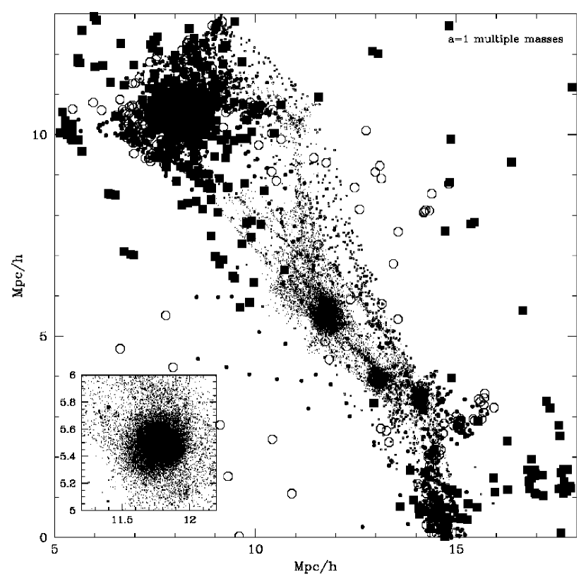
Figure 2: Distribution of particles of different masses in a thin slice through the center of halo A₁ (see Table 1) at $z=10$ (top panel) and at $z=0$ (bottom panel). To avoid crowding of points the thickness of the slice is made smaller in the center (about 30$h^{-1}$kpc) and larger (1$h^{-1}$Mpc) in the outer parts of the forming halo. Particles of different mass are shown with different symbols: tiny dots, dots, large dots, squares, and open circles.

After the initial conditions are set, we run the simulation again allowing the code to perform mesh refinement based only on the number of particles with the smallest mass.

2.3 Numerical simulations

We simulated a flat low-density cosmological model ($\Lambda$CDM) with $\Omega_{0}=1-\Omega_{\Lambda}=0.3$, the Hubble parameter (in units of $100{\rm\ kms^{-1}Mpc^{-1}}$) $h=0.7$, and the spectrum normalization $\sigma_{8}=0.9$. We have run two sets of simulations. The first set used $128^{3}$ zeroth-level grid in a computational box of $30\mbox{$h^{-1}$Mpc}$. The second set of simulations used $256^{3}$ grid in a $25\mbox{$h^{-1}$Mpc}$ box and had higher mass resolution. In the simulations used in this paper, the threshold for cell refinement (see above) was low on the zeroth level: $n_{\rm thresh}(0)=2$. Thus, every zeroth-level cell containing two or more particles was refined. This was done to preserve all small-scale perturbations present in the initial spectrum of perturbations. The threshold was higher on deeper levels of refinement. For the first set of simulations it was $n_{\rm thresh}=2$ at the first refinement level and $n_{\rm thresh}=3$ for all higher levels. For the second simulation the thresholds were $n_{\rm thresh}=3$ and $n_{\rm thresh}=4$ for the first level and higher levels, respectively.

In addition to effects introduced by limited mass and force resolution, integration errors of particle trajectories may affect the innermost regions of halos. The local dynamical time for particles moving in these regions is quite short. For example, the period of a particle on a circular orbit of radius $1\mbox{$h^{-1}$kpc}$ around the center of halo A is only $0.5\%$ of the Hubble time. Therefore, if the time step is not sufficiently small, numerical errors in these regions will tend to grow. Even for small time steps errors exist and tend to alter the density distribution in the centers of halos over some limited range of scales.

All of our simulations were started at $z_{i}=60$ and the step in the expansion parameter was chosen to be $\Delta a_{0}=2\times 10^{-3}$ for particles located on the zeroth base grid. This gives about 500 steps for particles located in the zeroth level for an entire run to $z=0$. We have done a test run with twice smaller time step for a halo of mass comparable (but with smaller number of particles) to the mass of halos studied in this paper. We did not find any significant differences in the resulting halo profile. For both sets of simulations, the highest level of refinement was ten for the largest mass resolution, which corresponds to $500\times 2^{10}\approx 500,000$ time steps at the tenth refinement level. Some simulations were rerun with smaller number of particles. They did not reach the highest levels of refinement, and, thus, they had fewer steps. For example, halo D₂ has reached only 7 levels of refinement and had only $500\times 2^{7}\approx 64,000$ time steps.

In the following sections we present density profiles of four halos. The halo A was the only halo selected for re-simulation in the first set of simulations. It was relatively quiescent at $z=0$ and had no massive neighbors. The halo was located in a long filament bordering a large void and was about 10 Mpc away from the nearest cluster-size halo. After the high-resolution simulation was completed we found that the nearest galaxy-size halo was about 5 Mpc away. The halo had a fairly typical merging history with $M(t)$ track slightly lower than the average mass growth predicted using the extended Press-Schechter model. The last major merger event occurred at $z\approx 2.5$; at lower redshifts the mass growth (the mass in this time interval has grown by a factor of three) was due to slow and steady mass accretion.

The halos B, C, and D were identified in the second set of simulations and were selected among halos residing in a well defined filament. Two of the halos (B and C) are neighbors located about 0.5 Mpc from each other. The third halo was 2 Mpc away from this pair. Thus, the halos were not selected to be too isolated as was the case in the first set of runs. Moreover, the simulation was also analyzed at both $z=0$ and at $z=1$ (when halos are more likely to be less relaxed). Therefore, the halo A can be considered as an example of a rather isolated well-relaxed halo. In many respects, this halo is similar to halos simulated by other research groups that used multiple mass resolution techniques. The halos B, C, and D from the second set of simulations can be viewed as representative of more typical halo population located in more crowded environments.

Parameters of the simulated dark matter halos are listed in Table 1. Columns in the table present (1) halo’s “name” (halos A₁, A₂, A₃ are the halo A re-simulated three times with different mass and force resolutions); (2) redshift at which the halo was analyzed; (3) the number of particles within the virial radius; (4) the smallest particle mass in the simulation; (5) formal comoving force resolution (cells size at the highest refinement level) achieved in the simulation.

Table 1: Simulation parameters

Halo	z	$N_{\rm part}$	$m_{\rm part}$	hformal
			$h^{-1}M_{\odot}$	$h^{-1}$kpc
(1)	(2)	(3)	(4)	(5)
A1	0	$1.2\times 10^{5}$	$1.6\times 10^{7}$	0.23
A2	0	$1.5\times 10^{4}$	$1.3\times 10^{8}$	0.91
A3	0	$1.9\times 10^{3}$	$1.1\times 10^{9}$	3.66
B1	0	$1.0\times 10^{6}$	$1.2\times 10^{6}$	0.10
B2	0	$1.5\times 10^{4}$	$1.2\times 10^{6}$	0.76
B3	1	$7.1\times 10^{5}$	$1.2\times 10^{6}$	0.19
C1	0	$1.1\times 10^{6}$	$1.2\times 10^{6}$	0.10
C2	0	$1.6\times 10^{4}$	$7.7\times 10^{7}$	0.76
C3	1	$5.0\times 10^{5}$	$1.2\times 10^{6}$	0.19
D1	0	$1.3\times 10^{6}$	$1.2\times 10^{6}$	0.10
D2	0	$2.0\times 10^{4}$	$7.7\times 10^{7}$	0.76
D3	1	$7.9\times 10^{5}$	$1.2\times 10^{6}$	0.19

3 Results

3.1 Comparison of the NFW and the Moore et al. profiles

Before we fit analytical profiles to profiles of simulated dark matter halos or compare them to the observed rotation curves, it is instructive to compare different analytical approximations. Although the NFW and Moore et al. profiles predict different behavior of $\rho(r)$ in the central regions of a halo, the scale at which this difference becomes significant depends on the specific values of the halo’s characteristic density and radius. Table 2 presents the parameters and statistics associated with the two analytical profiles. For the NFW profile more information can be found in Klypin et al. (1998), Łokas & Mamon (2000), and Widrow (2000).

Each profile is defined by two independent parameters. We choose these to be the characteristic density $\rho_{s}$ and radius $r_{s}$. In this case all expressions describing the properties of the profiles have a simple form and do not depend on the concentration. Both the concentration and the virial mass appear only in the normalization of the expressions. The choice of the virial radius (e.g., Łokas & Mamon 2000) as a scale unit results in more complicated expressions with explicit dependence on the concentration. In this case, one has to be careful about the definition of the virial radius, as there are several definitions in the literature. For example, it is often defined as the radius, $r_{200}$, within which the average density is 200 times the critical density. In this paper the virial radius is defined as the radius within which the average density is equal to the density predicted by the top-hat model: it is $\delta_{\rm TH}$ times the average matter density in the Universe. In the case of $\Omega_{0}=0.3$ models the virial radius defined in this way is about 30% larger than $r_{200}$ (e.g., Eke et al. 1998).

There is no unique way of defining a consistent concentration for the different analytical profiles. Again, it is natural to use the characteristic radius $r_{s}$ to define the concentration: $c\equiv r_{\rm vir}/r_{s}$. This simplifies the expressions. At the same time, if we fit the dark matter halo with the two profiles, we will get different concentrations because the values of the corresponding $r_{s}$ will be different. Alternatively, if we choose to match the outer regions of the profiles (say, $r>r_{s}$) as closely as possible, we may choose to change the ratio of the characteristic radii $r_{s,\rm NFW}/r_{s,\rm Moore}$ in such a way that both profiles reach the maximum circular velocity $v_{\rm circ}$ at the same physical radius $r_{\rm max}$. In this case, the formal concentration of the Moore et al. profile is 1.72 times smaller than that of the NFW profile. Indeed, with this normalization profiles look very similar in the outer parts as one finds in Figure 3. Table 2 also gives two other “concentrations”. The concentration $C_{1/5}$ is defined as the ratio of virial radius to the radius, which encompasses 1/5 of the virial mass (Avila-Reese et al. 1999). For halos with $C_{\rm NFW}\approx 5.5$ this 1/5 mass concentration is equal to $C_{\rm NFW}$. One can also define the concentration as the ratio of the virial radius to the radius at which the logarithmic slope of the density profile is equal to $-2$. This scale corresponds to $r_{s}$ for the NFW profile and $\approx 0.35r_{s}$ for the Moore et al. profile.

Table 2: Comparison of NFW and Moore et al. profiles

Parameter	NFW	Moore et al.
Density	$\rho=\frac{\displaystyle\rho_{s}}{\displaystyle x(1+x)^{2}}$	$\rho=\frac{\displaystyle\rho_{s}}{\displaystyle x^{1.5}(1+x)^{1.5}}$
$x=r/r_{s}$	$\quad\rho\propto x^{-3}$ for $x\gg 1$	$\quad\rho\propto x^{-3}$ for $x\gg 1$
	$\quad\rho\propto x^{-1}$ for $x\ll 1$	$\quad\rho\propto x^{-1.5}$ for $x\ll 1$
	$\quad\rho/\rho_{s}=1/4\phantom{string}$ at $x=1$	$\quad\rho/\rho_{s}=1/2\phantom{string}$ at $x=1$
Mass
$M=4\pi\rho_{s}r_{s}^{3}f(x)$	$f(x)=\ln(1+x)-\frac{\displaystyle x}{\displaystyle 1+x}$	$f(x)=\frac{2}{3}\ln(1+x^{3/2})$
$\phantom{string}=M_{\rm vir}f(x)/f(C)$
$M_{\rm vir}=\frac{4\pi}{3}\rho_{\rm cr}\Omega_{0}\delta_{\rm top-hat}r_{\rm vir}^{3}$
Concentration	$C_{\rm NFW}=1.72C_{\rm Moore}$	$C_{\rm Moore}=C_{\rm NFW}/1.72$
	for halos with the same $M_{\rm vir}$ and $r_{\rm max}$
$C=r_{\rm vir}/r_{s}$	$C_{1/5}\approx\frac{\displaystyle C_{\rm NFW}}{\displaystyle 0.86f(C_{\rm NFW})+0.1363}$	$C_{1/5}=\frac{\displaystyle C_{\rm Moore}}{[\displaystyle(1+C_{\rm Moore}^{3/2})^{1/5}-1]^{2/3}}$
	stringerror less than 3% for $C_{\rm NFW}=$5-30	string$\approx\frac{\displaystyle C_{\rm Moore}}{\displaystyle[C_{\rm Moore}^{3/10}-1]^{2/3}}$
	$C_{\gamma=-2}=C_{\rm NFW}$	$C_{\gamma=-2}=2^{3/2}C_{\rm Moore}$
		string$\approx 2.83C_{\rm Moore}$
Circular Velocity
$v_{\rm circ}^{2}=\displaystyle\frac{GM_{\rm vir}}{r_{\rm vir}}\frac{C}{x}\frac{f(x)}{f(C)}$	$x_{\rm max}\approx 2.15$	$x_{\rm max}\approx 1.25$
$\phantom{string}=\displaystyle v_{\rm max}^{2}\frac{x_{\rm max}}{x}\frac{f(x)}{f(x_{\rm max})}$	$v_{\rm max}^{2}\approx 0.216v_{\rm vir}^{2}\displaystyle\frac{C}{f(C)}$	$v_{\rm max}^{2}\approx 0.466v_{\rm vir}^{2}\displaystyle\frac{C}{f(C)}$
$v_{\rm vir}^{2}\phantom{.}=\displaystyle\frac{GM_{\rm vir}}{r_{\rm vir}}$	$\rho/\rho_{s}\approx 1/21.3$ at $x=2.15$	$\rho/\rho_{s}\approx 1/3.35$ at $x=1.25$

Figure 3 presents the comparison between the analytic profiles normalized to have the same virial mass and the same radius $r_{\rm max}$. We show results for halos of low and high values of concentration representative of cluster- and low-mass galaxy halos, respectively. The bottom panels show the profiles, while the top panels show the corresponding logarithmic slope as a function of radius. The figure shows that the two profiles are very similar throughout the main body of the halos. Only in the very central region do the differences become significant. The difference is more apparent in the logarithmic slope than in the actual density profiles. Moreover, for galaxy-mass halos the difference sets in at a rather small radius $\lesssim 0.01\mbox{$r_{\rm vir}$}$, which would correspond to scales $<1{\rm\ kpc}$ for the typical dark matter dominated dwarf and LSB galaxies. At the observationally interesting scales the differences between NFW and Moore et al. profiles are fairly small and the NFW profile provides an accurate description of the halo density distribution.

Note also that for galaxy-size (e.g., high-concentration) halos the logarithmic slope of the NFW profile has not yet reached its asymptotic inner value of $-1$ even at scales as small as $0.01\mbox{$r_{\rm vir}$}$. At this distance the logarithmic slope of the NFW profile is $\approx-1.4-1.5$ for halos with mass $\sim 10^{12}\mbox{$h^{-1}$M${}_{\odot}$}$. For cluster-size halos this slope is $\approx-1.2$. This dependence of the slope at a given fraction of the virial radius on the virial mass of the halo is very similar to the results plotted in Figure 3 of Jing & Suto (2000). These authors interpreted it as evidence that halo profiles are not universal. It is obvious, however, that their results are consistent with NFW profiles and the dependence of the slope on mass can be simply a manifestation of the well-studied $c_{\rm vir}(M)$ relation.

The NFW and Moore et al. profiles can be compared in a different way. We can approximate the Moore et al. halo of a given concentration with the NFW profile. Fractional deviations of the fits depend on the halo concentration and on the range of radii used for the fits. A low-concentration halo has larger deviations, but even for $C=7$ case, the deviations are less than 15% if we fit the halo at scales $0.01<r/\mbox{$r_{\rm vir}$}<1$. For a high-concentration halo with $C=17$, the deviations are much smaller: less than 8% for the same range of scales.

To summarize, we find that the differences between the NFW and the Moore et al. profiles are very small ($\Delta\rho/\rho<10\%$) for radii above 1% of the virial radius for typical galaxy-size halos with $C_{\rm NFW}\mathrel{\mathchoice{\lower 0.5pt\vbox{\halign{$\mathnew\displaystyle\hfil#\hfil$\cr>\crcr\sim\crcr}}}{\lower 0.5pt\vbox{\halign{$\mathnew\textstyle\hfil#\hfil$\cr>\crcr\sim\crcr}}}{\lower 0.5pt\vbox{\halign{$\mathnew\scriptstyle\hfil#\hfil$\cr>\crcr\sim\crcr}}}{\lower 0.5pt\vbox{\halign{$\mathnew\scriptscriptstyle\hfil#\hfil$\cr>\crcr\sim\crcr}}}}12$. The differences are larger for halos with smaller concentrations. In the case of the NFW profile, the asymptotic value of the central slope $\gamma=-1$ is not achieved even at radii as small as 1%-2% of the virial radius.

Figure 3: Comparison of the Moore et al. and the NFW profiles. Each profile is normalized to have the same virial mass and the same radius of the maximum circular velocity. Left panels: High-concentration halo typical of small galaxy-size halos $C_{\rm NFW}=17$. Right panels: Low-concentration halo typical of cluster-size halos. The deviations are very small ($<3\%$) for radii $r>r_{s}/2$. Top panels show the local logarithmic slope of the profiles. Note that for the high concentration halo the slope of the profile is significantly larger than the asymptotic value -1 even at very small radii $r\approx 0.01r_{\rm vir}$.

3.2 Convergence study

The effects of numerical resolution can be studied by resimulating the same objects with higher force and mass resolution and with a larger number of time steps. In this study we performed simulations of the same halos with increasingly higher mass resolution. In the ART code simulations the subsequent mesh refinements are done when particle density in a mesh cell exceeds a specified threshold. The mass resolution is thus tightly linked with the highest achievable spatial resolution.

Table 3 gives parameters of the halos and parameters of their fits. The first and the second columns give the halo name (Table 1) and the redshift at which the halo was studied. Columns (3-5) present virial mass, radius, and the maximum circular velocity of the halo. Columns (6-8) present parameters of the fits: the halo concentration as estimated using the NFW profile and the maximum relative errors of the NFW and Moore et al fits. The bottom panel in figure 4 shows density profiles for the simulations of halo A (see Table 1). Here, as in the Fig.1a in Moore et al. (1998), all profiles are plotted down to the formal force resolution of the corresponding run. Although it may appear that density profiles have not converged in the central region and that the low resolution simulations produce erroneous results, this is simply an artifact of plotting the profiles below the actual numerical resolution (or convergence scale). The top panel in figure 4 and figure 5 show profiles of halos A, B, C, and D plotted down to four formal resolutions of the simulations (4 mesh cells at the highest refinement level). The figures show that in this case density profiles in lower resolution simulations are in very good agreement with profiles in high-resolution runs at all radii. For example, there are no systematic differences in the logarithmic slope of the profile at a given distance and we find no significant change in the concentration parameters or the maximum circular velocities of halos (see Table 3).

Table 3: Halo parameters

Halo	z	$M_{\rm vir}$	$R_{\rm vir}$	$V_{\rm max}$	$C_{\rm NFW}$	RelErr	RelErr
		$h^{-1}M_{\odot}$	$h^{-1}$kpc	km/s		NFW	Moore
(1)	(2)	(3)	(4)	(5)	(6)	(7)	(8)
A1	0	$2.0\times 10^{12}$	257	247.0	17.4	0.17	0.20
A2	0	$2.1\times 10^{12}$	261	248.5	16.0	0.13	0.16
A3	0	$2.0\times 10^{12}$	256	250.5	16.6	0.16	0.10
B1	0	$1.2\times 10^{12}$	215	199.5	15.6	0.30	0.14
B2	0	$1.1\times 10^{12}$	213	205.0	16.5	0.15	0.14
B3	1	$8.5\times 10^{11}$	241	195.4	12.3	0.23	0.16
C1	0	$1.3\times 10^{12}$	225	190.6	11.2	0.29	0.23
C2	0	$1.2\times 10^{12}$	220	184.9	9.8	0.11	0.12
C3	1	$6.8\times 10^{11}$	208	165.7	11.9	0.37	0.20
D1	0	$1.5\times 10^{12}$	235	213.9	11.9	0.15	0.68
D2	0	$1.5\times 10^{12}$	234	216.8	13.4	0.10	0.09
D3	1	$9.6\times 10^{11}$	245	202.4	9.5	0.25	0.60

Closer examination of the bottom panel in Figure 4, shows that profiles have not converged at two formal resolutions. This is at odds with our convergence study in Kravtsov et al. (1998). We attribute this difference to the fact that mass resolution in the latter study was kept fixed when force resolution was varied. Our highest resolution run A₁, if considered including scales larger than two formal resolutions, is consistent with conclusion about the shallow central slope made in Kravtsov et al. (1998). Indeed, if the profiles are considered down to the scale of two formal resolutions (a scale smaller than the smallest converged scale), the density profile slope in the very central part of the profile $r\lesssim 0.01r_{\rm vir}$ is close to $\gamma=-0.5$. In light of the results shown in Figure 4, it is clear that this is an artifact of underestimating true convergence scale and conclusions about shallow central density distributions made in Kravtsov et al. (1998) are therefore incorrect.

Figure 4: Density profiles of halo A simulated with different mass and force resolutions. Bottom panel: The profiles are plotted down to the formal force resolution of each simulation. Because the plot shows results below the actual force resolution, one gets a wrong impression that the profile gets steeper and the concentration increases when the mass resolution is increased. Top panel: the profiles plotted down to four formal resolutions. For vastly different mass and force resolutions the convergence is reached at these scales. At the scale of a few percent of the virial radius the density profile is visibly steeper than the limiting slope $\gamma=-1$ of the NFW profile. This is consistent with the NFW profile for a halo of this concentration.

It is not clear which numerical effect determine the convergence scale. It is likely that this scale is determined by a complex interplay of all numerical effects. For the ART simulations we found empirically that the scale above which the density does not deviate (deviations were less than 10%) from results of higher resolution simulation is $\gtrsim 4$ formal force resolutions or containing more than 200 particles, whichever is larger. The limit very likely depends on particular code used and is not universal. Figure 4, top panel, shows that for the halo A, convergence for vastly different mass and force resolution is reached for scales $\gtrsim 4$ formal force resolutions (all profiles in this figure are plotted down to the radius of 4 formal force resolutions). For all resolutions, there are more than 200 particles within the radius of four resolutions from the halo center. For the highest resolution simulation (halo A₁) convergence is reached at scales $\gtrsim 0.005\mbox{$r_{\rm vir}$}$, assuming convergence at 4 times the formal resolution as found for halos A₂ and A₃. For halos B, C, D (figure 5) this criterion also worked, but was mostly defined by the number of particles (more than 200-300 particles for convergence).

Figure 5: Convergence of profiles for halos B, C, D. All the curves in this plot start at radii, which contain at least 200 particles and which are larger than 4 formal resolutions. For clarity, the profiles of halos C and B were shifted downwards by factors of 10 and 100, respectively. The full curves are for halos B₁, C₁, D₁, which have more than a million particles each. The dashed curves show profiles of halos B₂, C₂, D₂ with $(15-20)\times 10^{3}$ particles. The error bars indicate $2\sigma$ fluctuations of density at each radius due to moving satellites and residual oscillations inside the halos. The dispersion was estimated using density profiles at four time moments in the interval $z=0-0.03$ ($\approx 4\times 10^{8}$ yrs).

3.3 Halo profiles

In order to judge which analytical profile provides a better description of the simulated profiles we fitted the NFW and Moore et al. analytic profiles. Figure 6 presents results of the fits for halo A and shows that both profiles fit the simulated profile equally well: fractional deviations of the fitted profiles from the numerical one are smaller than 20% over almost three decades in radius. It is thus clear that the fact that the numerical profile has slope steeper than $-1$ at the scale of $\sim 0.01\mbox{$r_{\rm vir}$}$ does not mean that a good fit of the NFW profile (or even analytic profiles with shallower asymptotic slopes) cannot be obtained. Figure 7 shows the fitting of halos in the second set of simulations. Each halo in the plot has more than a million particles – ten times more than halo A. One would naively expect that this increase in the resolution should clearly show which profile makes a better fit. Indeed, more particles and better resolution gave smaller deviations, but the fits became better for both approximations. For example, at 1% of the virial radius of the halo D the deviations were 3.6% for the NFW profile and 6.2% for the Moore et al. profile – down from 20% for the halo A at the same distance. The Moore et al. approximation gave a better fit for halos B and C, but not for halo D. The NFW approximation was less accurate on intermediate scales around $(0.03-0.1)R_{\rm vir}$, but the errors were quite small. Thus, both approximations gave comparable results.

There is definitely a certain degree of degeneracy in fitting various analytic profiles to numerical results. Figure 8 illustrates this further by showing results of fitting profiles (solid lines) of the form $\rho(r)\propto(r/r_{0})^{-\gamma}[1+(r/r_{0})^{\alpha}]^{-(\beta-\alpha)/\gamma}$ to the same simulated halo profile (halo A₁) shown as solid circles. The legend in each panel indicates the corresponding values of $\alpha$, $\beta$, and $\gamma$ of the fit; the digit in parenthesis indicates whether the parameter was kept fixed ($0$) or not ($1$) during the fit. The two right panels show fits of the NFW and Moore et al. profile; the bottom left panel shows fit of the profiles used by Jing & Suto (2000). The top left panel shows a fit in which the inner slope was fixed but $\alpha$ and $\beta$ were fit. The figure shows that all four analytic profiles can provide a good fit to the numerical profile in the whole range of resolved scales: $0.005-1\mbox{$r_{\rm vir}$}$.

Figure 6: Fits of the NFW and Moore et al. halo profiles to the profile of halo A₁ (bottom panel). The top panel shows fractional deviations of the analytic fits from the numerical profile. Note that both analytic profiles fit numerical profile equally well: fractional deviations are smaller than 20% over almost three decades in radius.

As we mentioned in § 2.3, the halo A analyzed in the previous section is somewhat special because it was selected as an isolated relaxed halo. Halos, which are not very isolated and relaxed are also interesting. After all, they represent the majority of all halos. When we compare observed rotation curves of galaxies with predicted circular velocity curves of the halos, we do not know if the galaxy host halo is well relaxed or not. In order to reach unbiased conclusions, we will present analysis of halos from the second set of simulations at redshifts $z=0$ and $z=1$ (halos B_1,3, C_1,3, and D_1,3), which were not selected to be relaxed or isolated. Note that these halos did not have major mergers immediately prior to the epoch of analysis, which could produce large distortions of their profiles. Based on the results of the convergence study presented in the previous section, we will consider profiles of these halos only at scales above four formal resolutions and not less than 200 particles. There is an advantage in analyzing halos at a relatively high redshift. Halos of a given mass will have lower concentration (see Bullock et al. 2000). Lower concentration implies a large scale at which the asymptotic inner slope is reached.

Figure 7: Fits of the NFW (dotted curves) and Moore et al. (dot-dashed curves) profiles to the density distributions of halos B, C, D (solid curves) in the highest resolution run at $z=0$ (top left). For clarity, the profiles of halos C and B were shifted down by factors of 10 and 100, respectively. Error bars present $2\sigma$ fluctuations of density profiles at different time moments estimated over the last $\approx 4\times 10^{8}$yr of the run. Top right panel shows fractional deviations of the fitted profile from the simulated halo profile as a function of scale. The bottom panels show the same but for the halos B, C, and D at $z=1$. Note that halos at this redshift are not yet well relaxed as indicated by the density fluctuations in the peripheral parts of the profiles.

Figure 8: Analytic fits to the density profile of the halo A₁ from our set of simulations. The fits are of the form $\rho(r)\propto(r/r_{0})^{-\gamma}[1+(r/r_{0})^{\alpha}]^{-(\beta-\alpha)/\gamma}$. The legend in each panel indicates the corresponding values of $\alpha$, $\beta$, and $\gamma$ of the fit; the digit in parenthesis indicates whether the parameter was kept fixed ($0$) or not ($1$) during the fit. Note that various sets of parameters $\alpha$, $\beta$, $\gamma$ provide equally good fits to the simulated halo profile in the whole range resolved range of scales $\approx 0.005-1\mbox{$r_{\rm vir}$}$. This indicates a large degree of degeneracy in parameters $\alpha$, $\beta$, and $\gamma$

Figure 9: Circular velocity profiles for the halos B₁, C₁, and D₁ normalized to halo’s virial velocity. Halos are well resolved on all shown scales. Although the halos have very similar masses, the profiles are very different; the differences are due to real differences in the concentration parameters.

We found that substantial substructure is present inside the virial radius in all three halos at $z=1$. Figure 7 shows profiles of these halos at $z=0$ (top) and $z=1$ (bottom). The $z=0$ profiles are smoother than profiles at $z=1$. Note that bumps and depressions visible in the profiles have amplitude that is significantly larger than the shot noise. Halo C₃ appeared to be the most relaxed of the three halos. This halo had its last major merger somewhat earlier than the other two. Halo D₃ had a major merger event at $z\approx 2$. A remnant of the merger is still visible as a bump at $r\sim 100\mbox{$h^{-1}$kpc}$. The non-uniformities of profiles caused by substructure may substantially bias analytic fits if one uses the entire range of scales below the virial radius. Therefore, we used only the central, presumably more relaxed, regions in the analytic fits: $r<50\mbox{$h^{-1}$kpc}$ for halo D and $r<100\mbox{$h^{-1}$kpc}$ for halos B and C (fits using only central $50\mbox{$h^{-1}$kpc}$ did not change results).

The best fit parameters were obtained by minimizing the maximum fractional deviation of the fit: ${\rm max}[{\rm abs}(\log\rho_{\rm fit}-\log\rho_{\rm halo})]$. Minimizing the sum of squares of deviations ($\chi^{2}$), as is often done, can result in larger errors at small radii with the false impression that the fit fails because it has a wrong central slope. The fit that minimizes maximum deviations improves the NFW fit for points in the range of radii $(5-20)\mbox{$h^{-1}$kpc}$, where the NFW fit would appear to be below the data points if the fit was done by the $\chi^{2}$ minimization. For example, if we fit halo B by minimizing $\chi^{2}$, the concentration slightly decreases from 12.3 (see Table 1) to 11.8, the maximum error slightly increases to 27%, but the fit goes below the data points for most of the points at small radii.

We have also fitted density distribution of halo B assuming even more stringent limits on the effects of numerical resolution. We fitted the halo starting at the scale equal to six times the formal resolution, minimizing the maximum deviation. Inside this radius there were about 900 particles. Resulting parameters of the fit were close to those in Table 1: $C_{\rm NFW}=11.8$, and maximum error of the NFW fit was 17%.

We found that for halos B and C the errors in the Moore et al. fits were systematically smaller than those of the NFW fits, though the differences were not dramatic. But Moore et al. fit poorly in the case of halo D. It formally gave very small errors, but at the expense of unreasonably small concentration $C_{\rm NFW}=2$. When we constrained the approximation to have about twice larger concentration as compared with the best NFW fit, we were able to obtain a reasonable fit (this fit is shown in Figure 7). Nevertheless, the central density distribution is fit poorly in this case.

Therefore, our analysis does not show that one analytic profile is better then the other for description of the density distribution in simulated halos. Despite the larger number of particles per halo and the lower concentrations of $z=1$ halos, results are still inconclusive. The Moore at al. profile is a better fit to the profile of halo C; the NFW profile is a better fit to the central part of the halo D. Halo B represents an intermediate case where both profiles provide equally good fits (similar to the analysis of halo A). Remarkably, the same conclusions hold for the halo profiles at $z=0$.

Both at $z=0$ and $z=1$, there are real deviations in parameters of halos of the same mass. We find the same differences in estimates of $C_{1/5}$ concentrations, which do not depend on specifics of an analytic fit. The central slope at around $1{\ }\mbox{kpc}$ also changes from halo to halo. Halos B and C have the same virial radii and nearly the same circular velocities, yet their concentrations are different by 30%. Indeed, halos in the Table 3 have similar masses in the range $(1.2-2)\times 10^{12}\mbox{$h^{-1}$M${}_{\odot}$}$. If halos had a universal profile – a shape, which depends only on halo mass, then we should expect that the circular velocity curves are very similar for our halos. Figure 9 shows circular velocities for halos B, C, and D, which have only 25% deviations in their virial mass. The halos clearly do not have a universal one-parameter shape. There are substantial variations in the curves, which occur at relatively large radii ($\sim 0.1-0.3R_{\rm vir}$). The variations are due to differences in halo concentration – each curve is well described by a NFW or Moore et al. profile but their concentrations are somewhat different. Our three halos clearly constitute a small sample. Bullock et al. (2000) and Jing (2000) studied the spread of halo concentrations in a large sample of halos. For a given mass it was found that halos have 20-50% variations in the concentration at $1\sigma$ level, which is consistent with what we find for our halos.

4 Discussion and conclusions

We have analyzed a series of simulations with vastly different mass and force resolutions with the goal of studying density distribution in the central regions of galaxy-size dark matter halos. We used multiple mass simulations performed using the ART code; the simulations were performed with variable mass, force and temporal resolutions. In the highest resolution runs, we achieved a (formal) spatial dynamical range of $2^{18}=262144$; the simulation was run with 500,000 steps for particles at the highest level of refinement.

Using these simulations, we have studied convergence of halo density profiles for different mass and force resolutions. We show that the halo profiles converge at scales larger than a certain (true numerical resolution) scale defined by numerical effects. This scale is probably code dependent, but can be found for any numerical code by a convergence study. For the ART simulations presented here, the density profiles converged at the scale of four times the formal force resolution or the radius containing more than 200 particles, whichever is larger. In this sense, our results are consistent with results of the “Santa Barbara” cluster comparison project (Frenk et al. 1999): the density profiles of a cluster-size halo simulated with different numerical codes and resolutions agree with each other at all resolved scales.

In KKBP98 we have discussed convergence tests in which we varied force resolution while keeping mass resolution fixed. Using these tests we concluded that density profiles converge at radii twice the local formal resolution of a simulation. The convergence tests presented in this paper, however, show that mass resolution places more stringent conditions on the trustworthy range of scales. Although we can reproduce our previous results (shallower than $-1$ density profiles at radii of two formal resolution), our new convergence tests show that these results were affected by limited mass resolution. We conclude that we overestimated our force resolution KKBP98 and that the conclusions about the shallow central slopes presented there were an artifact of that overestimate. Other results in KKBP98 that focus on general halo characteristics, such as the scatter in profile shapes, and the agreement between the $V_{max}$ — $r_{max}$ relations of simulated dark halos and dark matter dominated dwarf and LSB galaxies, are valid.

At scales above four times the formal resolution and containing more than 200 particles results presented in this paper agree well with previous simulations. For example, the concentration parameter for the halos are in good agreement with the concentration-mass dependence ($c(M)$) presented in Bullock et al. (2000) based on the previous simulations.

We can also reproduce results of convergence studies by Moore et al. (1998) and Ghigna et al. (1999). At first glance it may appear that our conclusions are in direct contradiction with these studies that concluded that at least several millions of particles are needed to resolve a halo profile properly. However, the contradiction is only in interpretation rather than in the results themselves. For example, Figure 2 in Ghigna et al. shows a cluster profile simulated at 3 different mass and force resolutions. The conclusion the authors make based on this convergence study is (at least qualitatively) similar to our conclusion: the profiles converge at all mass resolutions at scales above $6\epsilon$, where $\epsilon$ is the spline force softening of their code (roughly equivalent to our formal resolution). Why is this criterion is more severe than ours? The obvious reasons are differences in the force shape and other differences between numerical codes. However, it appears that the softening in these simulations was set too low (the profiles were “overresolved”) and convergence scale is determined by the number of particles criterion rather than by force resolution. Indeed, we can estimate the number of particles within the softening scale in these simulations as $N_{p}(<\epsilon)\approx(4\pi/3)(\rho_{crit}/m_{p})(1+\delta)\epsilon^{3},$ where $\epsilon$ is the softening length, $m_{p}$ is the particle mass, $\rho_{crit}$ is the critical density, and $\delta$ is the overdensity reached at the softening scales. For the HIRES simulation in Ghigna et al., $\epsilon=0.5h^{-1}{\ }{\rm kpc}$ and $m_{p}=5.37\times 10^{7}h^{-1}{\ }{\rm M_{\odot}}$ and $\delta\sim(0.5\div 1.0)\times 10^{7}$, which gives $N_{p}(<\epsilon)\sim 10-30$. For their LOWRES simulation this number is even lower $\sim 5-10$. The scale containing $\gtrsim 200-300$ particles should be close to the convergence that is found in this study (e.g., $3-4\epsilon$ for the LOWRES run).

In light of these considerations, the profiles in Fig 2 of Moore et al. (1998) are perfectly consistent with each other if considered at scales $\gtrsim 4\epsilon$. Their results are thus perfectly consistent with our results and conclusions. One needs more particles only if the softening is set too small and the inner regions are over-resolved. In this case the true resolution is set by the radius that contains at least a couple hundred particles. The main point is that the higher mass resolution is needed to probe deeper into the inner regions of halos. However, if one is interested only in the profiles at, say, $r\gtrsim 0.02R_{vir}$ (sufficient to determine halo’s concentration, maximum circular velocity, etc.) than, as Figure 2 in Ghigna et al. (1999) and Figure 5 in this paper clearly show, $\sim(2-5)\times 10^{5}$ within the virial radius is adequate.

In this paper, we present results for halos that contain $1.2\times 10^{5}$ to $1.6\times 10^{6}$ particles within their virial radius. We show that for the galaxy-size halos ($M_{\rm vir}=7\times 10^{11}\mbox{$h^{-1}$M${}_{\odot}$}-2\times 10^{12}\mbox{$h^{-1}$M${}_{\odot}$}$ and $C=9-17$) both the NFW profile $\rho\propto r^{-1}(1+r)^{-2}$ and the Moore et al. profile $\rho\propto r^{-1.5}(1+r^{1.5})^{-1}$ provide fairly good fits of the simulated profiles with deviations of about 10% for radii larger than 1% of the virial radius. For dwarf and LSB galaxies commonly used for comparisons with model predictions, this corresponds to scales $\mathrel{\mathchoice{\lower 0.5pt\vbox{\halign{$\mathnew\displaystyle\hfil#\hfil$\cr>\crcr\sim\crcr}}}{\lower 0.5pt\vbox{\halign{$\mathnew\textstyle\hfil#\hfil$\cr>\crcr\sim\crcr}}}{\lower 0.5pt\vbox{\halign{$\mathnew\scriptstyle\hfil#\hfil$\cr>\crcr\sim\crcr}}}{\lower 0.5pt\vbox{\halign{$\mathnew\scriptscriptstyle\hfil#\hfil$\cr>\crcr\sim\crcr}}}}1$kpc. Therefore, the debate about which analytic profile provides a better description of the CDM halo profiles may well be irrelevant for comparisons to measured galaxy rotation curves. Such comparisons are also subject to other uncertainties, one of which is limited spatial extent of the observed rotation curves. The particular shape of the inner density distribution may be important for galaxy cluster observations, however. Cluster-size halos are predicted to have smaller concentrations, which means that the scale at which differences between the NFW and Moore et al. profiles become significant is larger and is observationally relevant.

These results are consistent with results of Moore et al. (1999) who found that galaxy-size halos in CDM models are well described by the $\rho\propto r^{-1.5}(1+r^{1.5})^{-1}$ profile. The authors used simulations of the standard CDM model with mass and force resolution similar to our simulations ($2\times 10^{6}{\ }M_{\odot}$ and $1$ kpc, respectively). They found that the NFW profile that was fitted at radii above $3\%$ of the halo’s virial radius, underpredicts the density at smaller radii by up to $20-30\%$. This is consistent with out results for halos B and C, although not for halo D, which probably indicates a certain degree of variance among profiles of halos of the same mass (Jing 2000; Bullock et al. 2000; Avila-Reese et al. 1999).

Jing & Suto (2000) simulated formation of galaxy-, group-, and cluster-size halos with resolution similar to our highest-resolution simulations. They also found that the NFW profile fit to the outer regions (radii above few percent of the virial radius) underestimates the density in the innermost regions of the halo. The degree of discrepancy, however, appears to be different for different halos (see their Fig. 2), which is consistent with our conclusions. The authors conclude that the shapes of the density profiles vary from galaxy- to group-, to cluster-size halos. However, as we argued in § 3.1, their results could be interpreted as the manifestation of concentration-mass relation instead.

Most recently, Fukushige & Makino (2001) simulated 12 halos with masses ranging from $4.3\times 10^{11}{\ }M_{\odot}$ to $7.9\times 10^{14}{\ }M_{\odot}$, again with resolution similar to the resolution of simulations presented here. The dependence of the inner logarithmic slope on the halo mass observed by Jing & Suto (2000) was not found in these simulations. Instead, the steepest slope of the density profiles was found to be close to $-1.5$ for all masses. This is surprising because such dependence is expected from the concentration-mass correlation (e.g., NFW; Bullock et al. 2000). It is not clear what could explain this discrepancy. Note also that setup of these simulations was somewhat different from the setup that is usually used: the simulations followed halo collapse from a spherically symmetric configuration centered on a gaussian density peak with no external tidal field included.

We show that density profiles of halos that are not fully relaxed may contain real non-uniformities due to substructure and differences in the density distributions. These non-uniformities affect the fit quality for a particular analytic profile and result in somewhat different values of fitted parameters (e.g., concentration). This was clearly seen at redshift $z=1$ for halos B,C,D (Figure 7), which by that time have not yet relaxed. At redshift $z=0$ the halos were much more quiet and the deviations from the fits were much smaller. It is interesting to note that the non-equilibrium effects do not qualitatively change the shape of the central parts of density profiles. For example, we found that at both redshifts the profile of halo C is best fit by the Moore et al. profile. The density profile of halo D, however, is best fit by the NFW profile again at both redshifts. Note that these three halos were simulated with the same mass and force resolution (indeed, in the same simulation). It seems that the main difference between these halos is their merger histories. We conclude, therefore, that differences in merger history and/or different degree of substructure in halos of the same mass may explain the scatter in profile shapes and concentration parameters found in previous studies (KKBP98; Jing 2000; Bullock et al. 2000).

In view of the current less confusing situation regarding the theoretical predictions for CDM profiles, it is interesting to discuss how the theory compares to observations. Rotation curves of a number of dwarf and LSB galaxies have recently been re-examined using H$\alpha$ observations and/or including corrections for beam-smearing in HI observations (e.g., Swaters, Madore & Trewhella 2000; van den Bosch et al. 2000). The results show that for the majority of galaxies, the H$\alpha$ rotation curves are significantly different in their central regions than the rotation curves derived from HI observations. This indicates that the HI rotation curves are affected by beam smearing (Swaters et al. 2000). This also implies that beam smearing may be at least partly responsible for the universal shape of the LSB rotation curves discussed in KKBP98.

It is possible that part of the discrepancy between the rotation curves of the different tracers may be due to real differences in the kinematics of the two gas components (ionized and neutral hydrogen). Preliminary comparisons between the new H$\alpha$ rotation curves and model predictions show that NFW density profiles are consistent with the observed shapes of the rotation curves (van den Bosch & Swaters 2000; Navarro & Swaters 2000). Moreover, cuspy density profiles with inner logarithmic slopes as steep as $\sim-1.5$ also seem to be consistent with the data (van den Bosch & Swaters 2000). A separate concern is not the shape of the inner density profile, but rather the value of the central density. There are indications that CDM halos are too concentrated (Navarro & Swaters 2000; McGaugh et al. 2000; Navarro & Steinmetz 2000; Firmani et al. 2000) in comparison with galactic halos. However, van den Bosch & Swaters (2000) have argued, based on detailed modeling of adiabatic contraction and beam-smearing, that dwarf galaxy concentrations are in fact consistent with the observed distribution in $\Lambda$CDM halos. Thus, although the shape of galactic rotation curves may be not as different from predictions as was thought before, the halo concentrations derived from observations are alarmingly low. The recent observational progress made in this field promises to resolve and clarify this issue in the near future. At larger scales ($r\gtrsim 100$ kpc), the constraints from weak galaxy-galaxy lensing (Fischer et al. 2000; Smith et al. 2000) should be very useful in constraining the overall profile and concentrations of galactic halos.

In summary, the study presented here is aimed to clarify the issue of convergence of the density profiles of CDM halos. We show that convergence can be reached regardless of the mass resolution, although the convergence scale does depend on the mass resolution: the higher mass resolution results in smaller convergence scale for the same objects, but it does not affect the outer parts of the profile. Our results also indicate that there is a real scatter in shapes of density profiles and halo parameters. Larger systematic studies currently underway may put these conclusions on a firmer footing.

References

- Avila-Reese et al. (1999) Avila-Reese, V., Firmani, C., Klypin, A.A., Kravtsov, A.V. 1999, MNRAS 310, 527
- Binney & Tremaine (1987) Binney, J., & Tremaine, S. 1987, Galactic Dynamics, Princeton: Princeton Univ. Press
- Bullock et al. (2000) Bullock, J.S., Kolatt, T.S., Sigad, Y., Somerville, R.S., Kravtsov, A.V., Klypin, A., Primack, J.P., Dekel, A. 2000, MNRAS submitted (astro-ph/9908159)
- Bullock, Kravtsov & Weinberg (2000) Bullock, J.S., Kravtsov, A.V., & Weinberg, D.H. 2000, ApJ 539, 517
- Eke et al. (1998) Eke, V.R., Cole, S., Frenk, C.S., & Henry, P.J. 1998, MNRAS, 298, 1145
- Firmani et al. (2000) Firmani, C., D’Onghia, E., Chincarini, G., Hernandez, X., Avila-Reese, V. 2000, MNRAS submitted (astro-ph/0005001)
- Fischer et al. (2000) Fischer, P. et al. 2000, AJ 120, 1198
- Flores & Primack (1994) Flores, R.A., & Primack, J.R. 1994, ApJ 427, L1
- Frenk et al. (1999) Frenk, C.S. et al. 1999, ApJ, 525, 554
- Fukushige & Makino (2001) Fukushige, T., & Makino, J. 2001, ApJ submitted (astro-ph/0008104)
- Ghigna et al. (1999) Ghigna, S., Moore, B., Governato, F., Lake, G., Quinn, T., Stadel, J. 1999, ApJ submitted (astro-ph/9910166)
- Jing (2000) Jing, Y.P. 2000, ApJ, 535, 30
- Jing & Suto (2000) Jing, Y.P. & Suto, Y. 2000, ApJ 529, L69
- Kauffmann et al. (1993) Kauffmann, G., White, S.D.M., & Guiderdoni, B. 1993, MNRAS 264, 201
- Klypin et al. (1998) Klypin, A., Gotlöber, S., Kravtsov, A.V., Khokhlov, A.. 1998, ApJ, 516, 530
- Klypin et al. (1999) Klypin, A., Kravtsov, A.V., Valenzuela, O., & Prada, F. 1999, ApJ, 522, 82
- Knebe et al. (2000) Knebe A., Kravtsov, A.V., Gottlöber, S., & Klypin A. 2000, MNRAS 317, 630
- Kravtsov (1999) Kravtsov, A.V. 1999, Ph.D. Thesis, New Mexico State University
- Kravtsov, Klypin & Khokhlov (1997) Kravtsov, A.V., Klypin, A., & Khokhlov, A.M. 1997, ApJS 111, 73
- Kravtsov et al. (1998) Kravtsov, A.V., Klypin, A., Bullock, J.S., & Primack, J.P. 1999, ApJ 502, 48
- Kravtsov & Klypin (1999) Kravtsov, A.V., & Klypin, A. 1999, ApJ 520, 437
- Łokas & Mamon (2000) Łokas, E.L., & Mamon, G. 2000, submitted to MNRAS, astro-ph/0002395
- McGaugh et al. (2000) McGaugh, S. et al. 2000, in preparation
- Moore (1994) Moore, B. 1994, Nature 370, 629
- Moore et al. (1998) Moore, B., Governato, F., Quinn, T., Stadel, J., Lake, G. 1998, ApJ 499, L5
- Moore et al. (1999) Moore, B., Quinn, T., Governato, F., Stadel, J., Lake, G. 1999, MNRAS 310, 1147
- Navarro et al. (1996) Navarro, J.F., Frenk, C.S., & White, S.D.M. 1996, ApJ 462, 563
- Navarro et al. (1997) Navarro, J.F., Frenk, C.S., & White, S.D.M. 1997, ApJ 490, 493
- Navarro & Steinmetz (2000) Navarro, J.F., & Steinmetz, M. 2000, ApJ 528, 607
- Navarro & Swaters (2000) Navarro, J.F., & Swaters, R.A. 2000, in preparation
- Smith et al. (2000) Smith, D.R., Bernstein, G.M., Fischer, P., Jarvis, R.M. 2000, ApJ submitted astro-ph/0010071
- Swaters et al. (2000) Swaters, R.A., Madore, B.F., Trewhella, M. 2000, ApJ 531, L107
- van den Bosch et al. (2000) van den Bosch, F.C., Robertson, B.E., Dalcanton, J.J., de Blok W.J.G. 2000, AJ 119, 1579
- (34) van den Bosch, F.C. & Swaters, R.A., 2000, AJ, submitted, astro-ph/0006048
- Widrow (2000) Widrow, L. 2000, submitted to ApJ., astro-ph/0003302