Dependence of Halo Properties on Interaction History, Environment and Cosmology

Abstract

I present results from numerical N-body simulations regarding the effect of merging events on the angular momentum distribution of galactic halos as well as a comparison of halo growth in Press-Schechter vs. N-body methods. A total of six simulations are used spanning 3 cosmologies: a standard flat $\Omega_{0}=1$ model, an open $\Omega_{0}=0.3$ model and a “tilted” flat $\Omega_{0}=1$ model with spectral index $n=0.8$. In each model, one run was conducted using a spatially uniform grid of particles and one using a refined grid in a large void. In all three models and all environments tested, the mean angular momentum of merger remnants (halo interaction products with mass ratios 3:1 or less) is greater than non-merger remnants. Furthermore, the dispersion in the merger-remnant angular momentum distribution is smaller than the dispersion of the non-merger distribution. The interpretation most consistent with the data is that the orbital angular momentum of the interactors is important in establishing the final angular momentum of the merger product. I give the angular momentum distribution which describes the merger remnant population.

I trace the most massive progenitor of $L_{*}$ galactic-mass halos (uniform grid) and $10^{11}M_{\odot}$ halos (refined void) from redshift $z=0$ back to $z=5$. Monte-Carlo mass histories match simulations reasonably well for the latter sample. I find that for halos of mass $10^{12}\mathrel{\hbox{\raise 2.15277pt\hbox{$<$}\hbox to0.0pt{\hss\lower 2.15277pt\hbox{$\sim$}}}}M\mathrel{\hbox{\raise 2.15277pt\hbox{$<$}\hbox to0.0pt{\hss\lower 2.15277pt\hbox{$\sim$}}}}10^{14}M_{\odot}$, this method can underestimate the mass of progenitors by 20%, hence yielding improper formation redshifts of halos. With this caveat, however, the general shapes of halo mass histories and formation-time distributions are preserved.

1 Introduction

The majority of spiral galaxies do not exist in isolation, but rather in an environment which sustains repeated close encounters and merging processes with both small and large companions (Schwarzkopf & Dettmar (2000)). Increasing evidence links disturbed or lopsided features of these galaxies to recent dynamical interactions. HST observations at high redshift have shown a preponderance of “train wreck” morphologies arising from major interactions. More recently, minor mergers have begun to be linked to $m=1$ mode disturbances as observed in the Fourier azimuthal decomposition of the galaxy’s surface brightness, generally denoted as “lopsidedness” (Rudnick, Rix, & Kennicut (2000); Rudnick & Rix (1998)). Specifically, studies by Richter & Sancisi (1994) have estimated that about half of late-type spirals exhibit significantly lopsided HI profiles, and half of these are field galaxies removed from cluster environments. Furthermore, Zaritsky & Rix find that 20% of all late-type spirals are significantly lopsided at optical and near-infrared wavelengths, yet have no obvious interactors. Rudnick & Rix (1998) find that one fifth of all disk galaxies, regardless of Hubble type, have azimuthal asymmetries in their stellar mass distribution. They also show that this observed asymmetry is in fact due to the underlying mass distribution and not dust obscuration or other non-dynamical effects. Dynamical profiles of this nature have been shown to be consistent with the accretion of a satellite galaxy of a larger system (Levine & Sparke (1998); Schwarzkopf & Dettmar (2000); and references therein). Consequently, it is probable that a substantial fraction of disk galaxies are experiencing interaction due to minor mergers.

Field spheroidals also have a number of properties such as shells, counterrotating inner disk, and bluer colors, which are believed to also be associated with recent merger events (de Carvalho & Djorgovski (1992); Rose et al. (1994); Longhetti et al. (1998); Abraham, et al. (1999)). By counting major mergers in large-scale simulations, Governato et al. (1999) show that a substantial fraction of the field elliptical population could be the result of major merging activity.

Hence, even in the field, observational evidence exists to support the hierarchical clustering scenario (HCS, see Peebles 1993) wherein larger objects are formed through the progressive assemblage of smaller mass collapsed structures. In short, the galaxy formation and evolution process is ubiquitously influenced by interactions. Therefore, to fully understand galactic formation and evolution and their consequences (both observational and theoretical), one must understand link between galaxy properties and interaction history, and how both of these may be modified by environmental effects.

The Press & Schechter formalism (1974, PS) is an analytical model to describe the hierarchical clustering scenario. The PS theory allows one to derive, in a relatively simple and straightforward way, the mass distribution of collapsed objects and its evolution with time in different FRW universes.

Despite its simple derivation, which relies uniquely on the linear theory, the PS formula captures the major feature of the hierarchical evolution as shown in the good fit of the PS mass function to N-body simulations (Frenk et al. (1988); Lacey & Cole (1994); Gardner et al. (1997); Borgani et al. (1999) and references therein). Recently it has become possible to pinpoint quantitative differences between this picture and the more complex N–body description. At cluster-sized masses, it is possible to match PS and simulated mass functions reasonably well (Governato et al. (1999); Borgani et al. (1999)), albeit with some tuning. However, at lower masses, evidence suggests that PS may provide a systematic overestimate of the halo number density (Bryan & Norman (1998); Gross et al. (1998); Tormen (1998)).

The PS formalism can be extended to give the probability that a halo of mass $M_{0}$ at redshift $z_{0}$ was also in a halo of mass $M_{1}$ at time $z_{1}$ (Bond et al. (1991)). This Extended Press-Schechter (EPS) can be further instrumented to construct halo formation times, mass histories, and merger rates in Monte-Carlo techniques (Lacey & Cole (1993)). Additional enhancements can be made which follow the detailed evolution and interaction of halos (Baugh et al. (1998) and references therein) in the form of semi-analytic merger trees (SAM) which are far less costly than N-body simulations. The SAM formalism has been used to predict a wide range of galaxy properties such as colors, morphology, merging history, and formation time (Baugh et al. (1996) and references therein). It has been used successfully to predict the same qualitative behavior found in N-body simulations. For instance, both SAM studies and N-body simulations find that the typical redshift of last major interaction of field ellipticals is lower than the cluster elliptical population (Governato et al. (1998); Baugh et al. (1996)). Furthermore, SAM results also generally reproduce observed behavior such as the morphology-density relation, color-magnitude diagrams, the Butcher-Oemler effect, and the luminosity evolution of color-selected galaxy samples (Kauffmann (1995); Kauffmann (1996); Kauffmann & Charlot 1998a ; Kauffmann & Charlot 1998b )

Given the great utility of PS methods, it is crucial to understand how the PS expression of structure formation relates to N-body simulations. PS predictions began to be tested against N-body results a number of years ago (Efstathiou et al. (1988); Lacey & Cole (1994)) and generally found, within the dynamic range of the simulations, to compare relatively well, although soon results were found that hinted at discrepancies between PS and simulations (Gelb & Bertschinger (1994)). As the range in masses accessible in the N-body method has increased, a number of other studies have been performed (Somerville et al. (2000); Tormen (1998); Sheth, Mo, & Tormen (1999); Borgani et al. (1999); Governato et al. (1999); Grammann & Suhhonenko (1999); Bryan & Norman (1998); Gross et al. (1998)). Somerville et al. (2000) compare the extended Press-Schechter model and find that, at high masses, discrepancies as high as 50% can exist between SAM and N-body predictions of progenitor numbers. They find discrepancies in such quantities as the PS mass function and conditional mass function, as well as SAM number-mass distributions. On the other hand, they find that a number of more relative quantities, such as the ratio of progenitor masses, are reproduced fairly well. Tormen (1998) also finds that EPS underpredicts the number of high-mass progenitors of cluster members at high redshift and concludes that caution should be exercised when modeling clustering properties of halo progenitors.

PS provides a representation of halos over a cosmologically representative range of environment. How applicable is the PS mass function in environmental extremes? Lemson & Kauffmann (1999) use N-body simulations to examine a number of halo parameters as function of environment. They find environmental dependence only for the mass distribution of halos, with angular momentum, concentration parameter, and formation time remaining unaffected. Consequently, one would expect PS to maintain as accurate a representation of environmental extremes as it does more representative regimes. In this work, I compare PS output to N-body simulations in both a representative volume and an extremely underdense region.

One quantity which cannot be derived from semi-analytic modeling is the angular momentum properties of a halo. Workers who study structure within galactic halos may derive halo mass and interaction histories from PS based methods, but spin parameters are typically assigned from the prescriptions found by previous N-body work. For example, Dalcanton, Spergel, & Summers (1997) use PS in combination with the spin parameter distribution of Warren et al. (1992) in order to study the distributions of surface brightness and scale length in disk galaxies. Van den Bosch (1998) uses this same distribution to examine the formation of disks and bulges within dark matter halos. Mo, Mao & White (1998) examine the formation of disk galaxies by incorporating an a priori distribution of dark matter halo angular momentum. Any SAM investigation of galaxy evolution and interaction (e.g. Somerville & Primack (1999)) must also assign spin parameters in this manner. When a halo experiences a major merging event, a new spin parameter can be assigned. However, should it be taken from the same general distribution found in N-body simulations or are the angular momenta of merger remnants systematically different from the quiescent population?

This paper is divided into two major thrusts. In the first, I examine the distribution of halo spin parameters in the overall halo population as well as merger remnants. I do this for several cosmologies, and for a large cosmologically representative volume (“uniform volume”) as well as a large, underdense void. In the second thrust, I compare semi-analytic halo progenitor masses and halo formation times to N-body simulations. I examine this relation in 3 uniform volumes and two voids, which collectively sample 3 different cosmologies.

2 Methods

2.1 The PS formalism

The standard PS formula predicts the number density $N(M,z)\,dM$ of high contrast structure of a given mass $M$ at a given epoch. The counting of such structures is based on the hypothesis that the overdense regions in the initial density field filtered on the scale of interest, will eventually collapse to form high contrast structure. Then to obtain the fraction of the mass collapsed on a certain scale, it needs to single out volumes of the filtered density field, where the (linearly) evolved density contrast $\delta$ exceeds a nominal threshold $\delta_{c}$ depending on the epoch, which guarantees that the associated volume is collapsed into a virialized object. The PS formula states:

$$N(M,z)~{}dM=\sqrt{2\over\pi}~{}{\rho_{0}\over M}~{}{\delta_{c}\over\sigma^{2}(M)}e^{\delta_{c}^{2}/2\sigma^{2}(M)}~{}{d\sigma(M)\over dM}~{}dM,$$ (1)

where $\sigma^{2}(M)$ is the mass variance of the perturbation field on the mass scale $M$:

$$\sigma^{2}(M)={1\over 2\pi^{2}}\int P(k)W^{2}(kR)k^{2}dk,$$ (2)

where $P(k)$ is the power spectrum and $W(kR)$ the Fourier transform if the real-space top-hat function. The conventional way to normalize the power spectrum is $\sigma_{8}$, the rms value of the linear fluctuation in the mass distribution on scales of $R=8\,h^{-1}$ Mpc. The field is taken to be Gaussian, and then the variance $S=\sigma^{2}(M)$ completely describes the density perturbation field. The threshold $\delta_{c}$ refers to the collapse of homogeneous spherical volumes and is found to be $\delta_{c}(z=0)=1.68$ for $\Omega_{0}=1$ models. The time variation of $\delta_{c}(z)$ is proportional to the linear growth factor $D(t)$ (see e.g. Peebles 1993) and contains the dependence from the specific FRW model. The overall normalization is such that at any $z$ all the available mass density $\rho$ resides in collapsed objects. For a detailed derivation and the analysis of the underlying statistics, see Bond et al (1991).

Paulo Tozzi graciously furnished the author with a copy of his code, an implementation of the Monte-Carlo method given in Lacey & Cole (1993) which is in turn based on the EPS “excursion set” formalism developed by Bond et al. (1991). In this method, the linear density field is smoothed at progressively larger mass scales and the mass of the halo containing a given particle at time $t_{1}$ is equal to the mass $M_{1}$ of the largest sphere which in which the average overdensity $\delta_{c}(t_{1})$ exceeds the collapse threshold. This ensures that a halos of mass $M$ has not yet been subsumed by a larger mass halo. $\delta_{c}(t)$, of course, changes with time and thus at later times, our halo of mass $M_{1}$ and time $t_{1}$ may ultimately become part of a larger collapsed structure $M_{2}$ which does not reach critical density until time $t_{2}$. By examining the growth of linear modes in the same region, one can statistically construct halo growth and interaction histories. Tozzi’s method differs from that of Lacey & Cole (1993) in the specifics of how it calculates the relationship between mass ($M_{1},M_{2}$, …) and collapse threshold ($\delta_{c}(t_{1}),\delta_{c}(t_{2})$, …) but yields essentially the same results (Tozzi, private communication). The method is described in detail by Governato & Tozzi (2001).

2.2 Simulations

I present 6 simulations which are evolved from 3 cosmological models: a critical universe (SCDM) ($\Omega_{0}=1$, $h\equiv H_{0}/100$ km s^-1 Mpc${}^{-1}=0.5$, $\sigma_{8}=0.7$), an open (OCDM) universe ($\Omega_{0}=0.3$, $h=0.75$, $\sigma_{8}=1$) and a tilted critical model (TCDM) with h$=0.5$, $\sigma_{8}=0.6$, a primordial index n$=0.8$ and a gamma factor $\Gamma=$ 0.37. The transfer function of Bardeen et al. (1986) was used in all cases. The simulated volume was 100 Mpc on a side (h already included) in all six runs. The parameters of the TCDM model have been chosen to satisfy both the cluster abundance and the COBE normalization at very large scales (Cavaliere, Menci, & Tozzi (1998)). This model differs from the SCDM in having less power and a steeper power spectrum at scales under 8h^-1 Mpc in comparison with the other two models. Each simulation was performed using PKDGRAV (Stadel & Quinn, in preparation) a parallel N–body treecode supporting periodic boundary conditions. All runs were started at redshifts sufficiently high to ensure that the absolute maximum density contrast $|\delta|\mathrel{\hbox{\raise 2.15277pt\hbox{$<$}\hbox to0.0pt{\hss\lower 2.15277pt\hbox{$\sim$}}}}1$. All simulations were evolved using between 500 and 1000 major time steps in which the forces on all particles were calculated. Each major time step is divided into a number of smaller substeps, the exact number of which is adaptively chosen by PKDGRAV such that all particles are moved on steps consonant with their dynamical times.

One simulation in each cosmology (the “uniform volume”) was run beginning from a spatially uniform grid of $144^{3}$ ($\sim$ 3 million) equal–mass particles with spline softening set to 60 kpc, allowing us to resolve individual halos with present-day circular velocities $V_{c}$ as low as 130 km s^-1 with 100 particles in OCDM and 170 km s^-1 with 100 particles in SCDM and TCDM. The particle masses were $1.57\times 10^{10}$ M_⊙ in OCDM and $2.32\times 10^{10}$ M_⊙ in SCDM and TCDM, while the opening angles of the SCDM and OCDM simulations were $\theta=0.5$ for redshifts $z>2$ and $\theta=0.7$ thereafter. TCDM was run with $\theta=0.5$ at all redshifts.

The remaining three simulations, one in each cosmology, were of a large void approximately 40 Mpc in diameter, where I defined the void region as the largest sphere that could be drawn in the simulation volume with mean overdensity $\bar{\delta}=-0.9$. The radii of the resultant spheres were 18.5 Mpc, 17 Mpc, and 13.5 Mpc for SCDM, OCDM and TCDM cosmologies respectively. The void runs were performed using the hierarchical grids technique in which the void region is represented with large numbers of low-mass particles, while the surrounding environment is composed of small numbers of high-mass particles. This allows much greater mass resolution to be achieved while ensuring that cosmological context is maintained. I used approximately 5 million particles in each void simulation, with an effective resolution of $432^{3}$ across the 100 Mpc box. $\theta$ was set to 0.6 for $z>2$ and 0.8 thereafter. Particles were spline-softened to 6.67 kpc, being $8.6\times 10^{8}$ M_⊙ in mass in critical models and $5.8\times 10^{8}$ in OCDM. Thus, structure in the voids was resolved in mass at a factor of 27 superior to the uniform volume runs. For convenience, I shall adopt the notation of SCDMu, OCDMu and TCDMu for the uniform volumes and SCDMv, OCDMv and TCDMv for the voids.

Throughout the paper, I identify halos using two primary methods. The first is the classic friends-of-friends (FOF) method (Davis et al. (1985)) using a linking length that corresponds to the mean interparticle separation at the density contour defining the virial radius of an isothermal sphere: $b=(n\rho_{vir}(z)/\bar{\rho}(z)/3.0)^{-1/3}$ where $n$ is the particle number density and $\rho_{vir}(z)$ is the virial density which depends on cosmology and is given in Kitayama & Suto (1996). The second is a variant of the spherical overdensity (SO) technique (Lacey & Cole (1994)) where I determine the most bound particle in a FOF group and find the radius from that particle at which the enclosed density crosses the virial threshold $\rho_{vir}(z)$.

2.3 Halo Mass Histories

In the simplest test between PS and N–body simulations, one assumes as input the spectral parameter $P(k)$ and $\sigma_{8}$, and compares the mass distribution at a given epoch. This essentially decides whether the PS formula correctly states the shapes and the normalization of the mass distribution of collapsed objects. Work has been done comparing the PS mass function to N-body simulations (Lacey & Cole (1994), Borgani et al. (1999), Governato et al. (1999), Bryan & Norman (1998), Gross et al. (1998), Tormen (1998)), and I do not use this method in my analysis.

I focus on another test which examines the evolution of the linear density field and compares it to the hierarchical clustering paradigm (cf. Kaiser (1986)) as realized in the N-body method. The parameter $\delta_{c}$ (cf. equation (1)) is the value of linear overdensity above which a perturbation is considered to be collapsed (evolved to the present day). Thus, $\delta_{c}$ determines the mapping between the linear perturbation field and the mass of a halo. By demanding that the $z=0$ PS mass function matches the z=0 mass function of the simulation, one is effectively anchoring $\delta_{c}$. This corresponds to the method used by Tormen (1998) in examining the conditional mass function of the calibrated EPS method. Thus there are no remaining free parameters to the evolution of the density perturbation field unless one invokes a $\delta_{c}(z)$ which varies non-linearly with redshift such as the one examined by Governato et al (1999).

In the uniform volume simulations, I identified all halos at z=0 of at least mass $M_{res}=2.318\times 10^{12}$ M_⊙, which corresponds to 100 particles in the flat models and roughly 150 in OCDM. With a mass-based cutoff, it is more straightforward to compare time evolution of the different cosmologies. Having at least 100 particles also insures that the halos are substantially larger than their softening lengths, guarding against the influence of numerical effects on global halo properties. I then “traced” each identified halo backwards in time, following the mass of the most massive progenitor as a function of redshift. In the case of the void runs, I identified all groups with at least 50 particles and traced them in a manner identical to the uniform volume counterparts. Unfortunately, the TCDM cosmology forms structure extremely late, and the void had only 12 halos in it greater than this mass cutoff. I therefore drop TCDMv from the following analysis.

I now wish to construct a Monte-Carlo realization which most accurately compares against the simulated results. Comparing individual halos is fruitless, given the extreme variation of mass histories even between halos of the same mass. Instead I wish to characterize the mean mass history of the sample, i.e. the average mass of a halo in the sample as a function of redshift. This was easily done by drawing the mass distribution of the halos to be modeled from the simulations themselves. Specifically, for each $M>M_{res}$ halo in a simulation, 100 Monte-Carlo realizations of the mass history of that halo were constructed. Thus, I can directly compare the aggregate mass history of the sample of simulated halos to the collective mass history of the Monte-Carlo realizations.

Errors in both simulated and Monte-Carlo samples were estimated using the bootstrap method. For each sample, 1000 identically-sized subsamples of halos were drawn from the z=0 distribution. Then, for each subsample, the mean mass history was calculated and used in the bootstrap estimate.

2.4 Halo Angular Momentum

For SCDMu and OCDMu uniform volumes and for the OCDMv void, I determine the distribution of halo spin parameters $\lambda=LE^{1/2}/GM^{5/2}$ for recent merger remnants versus non-remnants, where $E$ is the total energy of the halo, $L$ the angular momentum, and $M$ the mass. I select halos for this analysis based on particle number in the $z=0$ FOF group: 100 particles for SCDMu and OCDMu and 50 particles for OCDMv. The OCDMu particle cutoff is lower than in the section 2.3 for more favorable number statistics. To identify mergers, I use the groups determined by SKID, a halo-finding algorithm based on local density maxima. The SKID algorithm is similar to the DENMAX scheme (Gelb & Bertschinger, 1994) as it groups particles by moving them along the density gradient to the local density maximum. The density field and density gradient is defined everywhere by smoothing each particle with a cubic spline weighting function of size determined by the distance encompassing the nearest 32 neighbors. At a given redshift, only particles with local densities greater than one-third of 177 times the critical density are “skidded” to the local density maximum. This threshold corresponds roughly to the local density at the virial radius. The final step of the process is to remove all particles that are not gravitationally bound to their parent halo. SKID was originally designed to find high contrast density structures within larger halos (see Ghigna et al. (1998) for a more complete description). For halos with no resolved internal substructure (i.e. no halos within halos) it gives results very similar to FOF. However, SKID does not suffer of the well known pathology of FOF of linking together close binary systems (Governato et al. (1997)). Instead, it only combines two “clumps” of substructure when they are mutually gravitationally bound and thus is well suited for the task of identifying binary systems in the process of merging.

I denote a halo as a merger remnant if, at some time during $0<z<z_{m}$ it was classified as a single SKID group in one output, but two separate groups with a mass ratio $\leq 3:1$ in the preceding output. This method is essentially independent of output spacing except in the extreme case where the halo mass does grows quiescently by order its own mass between outputs. $z_{m}$ was chosen to be as close to $z=0.5$ as the outputs would allow. In SCDMu this is $z_{m}=0.4$, and in both OCDM runs $z_{m}=0.5$.

I use SKID to identify halos before the merging event and spherical overdensity to identify the descendant halo at the present time. The SO method has the advantage of culling out pathologically shaped groups which depart substantially from the isothermal sphere model. The most common example is a “dumbbell” halo, which consists of two spherical halos that FOF links together by a thin bridge of particles spaced close to $\rho_{vir}(z)/3$. The total spin parameter of such a configuration is irrelevant to this study which is concerned only with cases where the angular momentum of a galaxy is linked to its parent halo. The spin parameter $\lambda$ is calculated by considering the contributions of all particles within the SO virial radius. If I use the FOF group membership rather than the SO, the angular momenta for non-pathological cases (about the FOF center of mass) is generally the same. Strangely-shaped groups are in the minority and hence even with their addition in the FOF sample, the the results remain qualitatively similar.

3 Results

3.1 Angular Momentum of Merger Remnants

Figure 1: Distribution of spin parameters in flat and open uniform volumes, SCDMu and OCDMu, as well as the open-model void, OCDMv. Histograms depict the simulated data and curves show the best fit lognormal function as defined in equation 3. Dashed lines represent halos which have experienced no major merger since $z=0.5$ ($z=0.4$ in SCDMu), whereas solid lines depict the merger remnants. Since the void run contains relatively few halos, the spin parameters distribution is also shown in log space, where it should be Gaussian. Table 1 details fit and distribution parameters.

The halo spin parameter distribution in simulations is found to be well approximated by the lognormal function

$$p(\lambda){\rm d}\lambda={1\over\sigma_{\lambda}\sqrt{2\pi}}\exp\biggl{(}-{{\rm ln}^{2}(\lambda/\bar{\lambda})\over 2\sigma^{2}_{\lambda}}\biggr{)}{{\rm d}\lambda\over\lambda}$$ (3)

(van den Bosch (1998); Barnes & Efstathiou (1987); Ryden (1998); Cole & Lacey (1996); Warren et al. (1992)). Figure 1 shows $p(\lambda){\rm d}\lambda$ of simulated halos above $M_{res}$ at z=0. The solid histograms denote the merger-remnant population and the dotted histograms are halos which have not experienced a major merger since $z=z_{m}\sim 0.5$. The smooth curves are fits of the form in equation 3 to the simulated distribution. Parameters for the fits are given in Table 1. Since the OCDM void model contains so few halos, it is easier to see the details of the distributions by viewing them in log space in Figure 1d, where the fitting function is a Gaussian. It should be noted that Lemson & Kauffmann (1999) find no environmental dependence of spin parameter on environment. Hence, any differences in OCDMu vs. OCDMv arise from the fact that the simulations sample substantially different ranges in mass and not from environmental effects.

N-body results are often used to provide an angular momentum distributions for galaxy halos in semi-analytic models (Dalcanton et al. 1997; Mo et al. 1998; van den Bosch (1998)). Warren et al. (1992) find that the general distribution of halos peaks around $\bar{\lambda}=0.05$ with $\sigma_{\lambda}=0.7$, although later N-body researchers find distributions more consistent with $0.04\mathrel{\hbox{\raise 2.15277pt\hbox{$<$}\hbox to0.0pt{\hss\lower 2.15277pt\hbox{$\sim$}}}}\bar{\lambda}\mathrel{\hbox{\raise 2.15277pt\hbox{$<$}\hbox to0.0pt{\hss\lower 2.15277pt\hbox{$\sim$}}}}0.05$ and $\sigma_{\lambda}\approx 0.5$ (Cole & Lacey (1996); Mo, Mao, & White (1998); see also Steinmetz & Bartelmann (1995); Catelan & Theuns (1996)). I find $\sigma_{\lambda}$ of all halos (in the uniform volumes) lower than 0.6 with the merger remnant population tending lower still, while the peak of the all three simulations presented is $\bar{\lambda}\sim 0.035$. Hence, my results for the global halo population are in concordance with previous findings.

I find that in all cases the distribution of spin parameters of merger remnants is greater than non-merger remnants. The K-S probabilities that the two sets were drawn from the same distribution are given as $P_{KS}$ in Table 1 and are quite low. The K-S test is most certain in SCDMv, given the large number of major mergers. Even though both OCDM runs contain fewer resolved merger remnants, the K-S test differentiates the merger and non-merger remnant populations at substantial confidence. To determine the robustness of the dissimilar means $\bar{\lambda}$ of distributions, I use the Wilcoxon test (cf. Lupton 1993). The value $P_{Wil}$ given in Table 1 is the probability that the difference between the mean of the merger population the mean of the non-merger population could have occurred by chance. In all cases, the probability is quite high that $\bar{\lambda}$ of the two distributions are indeed significantly different. Consequently, spin parameters of halos which have experienced a recent major merger are distributed differently than halos which have not undergone a recent significant interaction.

Angular momentum has been found to be relatively insensitive to cosmology and collapse anisotropy for halos formed by less violent collapse, with the spread in $\bar{\lambda}$ arising mainly from tidal effects (Huss, Jain, & Steinmetz (1999)). This view is supported by Nagashima & Gouda (1998) who, using semi-analytics (the “merging-cell model”), find that the orbital angular momentum of major mergers is not important for the remnant, and that major merging activity as a whole has little effect on the halo angular momentum distribution. Given the large spread in $\bar{\lambda}$ in my results, it seems tempting to conclude that on a halo-by-halo basis, tidal effects are more important than merger history in determining the ultimate angular momentum of a halo. Merging may be looked at simply as adding a small upward bias. However, one should note that the dispersion $\sigma_{\lambda}$ in the merger remnants is typically lower than the non-merger remnants. This can imply one of two possibilities: A) the angular momentum of mergers is largely independent of tidal torques, depending more on the mergers themselves or B) merging adds selects for specific environments. In B), by considering mergers, we are simply biasing ourselves toward examining halos which are in a region that promotes merging, nurturing halos with a narrower range in $\lambda$ and a higher mean. In A), it is a combination of the orbital angular momentum of the merger and the spin-alignment of the halos that determines a remnant’s resultant angular momentum. However, if the spin-alignment were dominant, one would expect the dispersion in $\lambda$ to be larger than the non-merger distribution, as two average halos can either add their spins or have them cancel completely. Consequently in case A), the orbital angular momentum of merging halos is the more likely contributor to the final remnant momentum. To summarize, tidal effects can dominate the merger remnant angular momentum distribution only if the lower dispersion of the merger remnant population can be explained. A likelier explanation is that by examining mergers, one is merely selecting a specific environment and hence only a subset of the possible tidal torques. The equally likely alternative is that the orbital angular momentum of the pre-merger halos dominates the spin parameters of merger remnants.

How relevant is the contribution of mergers to the overall spin parameter distribution? Figure 2 plots the fraction of halos in my sample with spin parameters $\lambda$ that are major merger remnants. The result is strongly dependent on cosmology, given that in open universes, merging activity at low redshift is substantially less likely than in $\Omega_{0}=1$ models (Governato et al. (1998)). Consequently, the global effect of merging on halo angular momentum is simply determined by the rate of major mergers. This information is, however, of marginal utility since galaxy history or properties are rarely used to infer angular momentum. In general, the distribution $p(\lambda)d\lambda$ is employed in an a priori manner. In this case, researchers may wish to adopt a different distribution for galaxies which are merger remnants and those which are not.

The overall implication of these results is that merging activity is correlated with higher angular momentum. Orbital angular momentum of interaction halos would seem to be the cause most consistent my data. However, on galaxy scales, the angular momentum of ellipticals is generally much lower than spirals (Nagashima & Gouda (1998)). This is troublesome if ellipticals are to be considered merger remnants and spirals the results of long periods of quiescence. The quiescent accretion required to form a higher-$\lambda$ spiral disk would appear to take place in halos with systematically lower spin parameters. Differences in angular momenta between galaxy morphologies may be more due to formation epoch (Huss, Jain, & Steinmetz (1999)) than merger history.

Figure 2: The probability $P_{M}$ that a halo with a given spin parameter $\lambda$ is a merger remnant for SCDMu (solid line) and OCDMu (dotted line).

	All Halos				Merger Remnants				Non-Merger Remnants
Model	$N$	$\bar{\lambda}$	$\sigma_{\lambda}$		$N$	$\bar{\lambda}$	$\sigma_{\lambda}$		$N$	$\bar{\lambda}$	$\sigma_{\lambda}$	$P_{KS}$	$P_{Wil}$
SCDMu	1353	0.0366	0.585		261	0.0438	0.500		1092	0.0351	0.596	$10^{-7}$	$10^{-7}$
OCDMu	1609	0.0353	0.568		15	0.0492	0.278		1594	0.0352	0.569	0.0119	$10^{-3}$
OCDMv	94	0.0331	0.660		7	0.0495	0.657		87	0.0320	0.653	0.320	0.132

Table 1: Details of the halo spin parameter distribution for the sample of all halos, merger remnant halos, and non-merger remnant halos. $N$ denotes the number of halos in each distribution. The fitting parameters $\bar{\lambda}$ and $\sigma_{\lambda}$ for the lognormal distribution $p(\lambda)d\lambda$ are defined in equation 3. $P_{KS}$ is the K-S probability that the merger and non-merger populations were drawn from the same distribution. $P_{Wil}$ is the Wilcoxon probability that $\bar{\lambda}$ of the merger and non-merger populations occurred by chance.

3.2 Halo Mass Histories and Formation Times

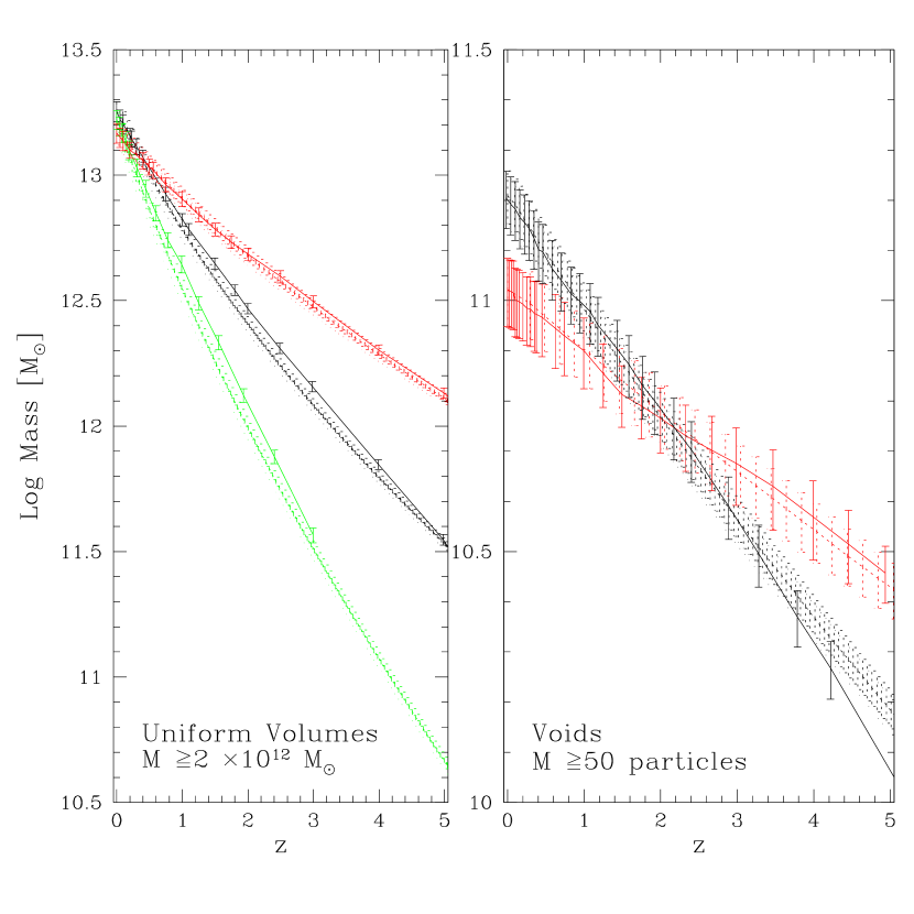
Figure 3: Average most massive progenitor mass vs. redshift $z$. The solid curves denote the average mass of the most massive progenitor of all halos in the simulations greater than the mass cut $M\geq 2\times 10^{12}M_{\odot}$ (uniform volumes, left panel) or $M>$ 50 particles (voids, right panel). The dashed curves are the Monte-Carlo realizations of the same sample of halos. The errorbars for all curves at the $1-\sigma$ deviations of 1000 bootstrap samples of the $z=0$ halo sample. In the left panel, each pair of curves (i.e. one dashed and one solid) represents a different cosmology from top to bottom view at $z=5$: OCDMu, SCDMu, TCDMu. In the right panel, the steep pair of curves denotes the SCDMv run, and the shallower the OCDMv run.

Here I compare the Monte-Carlo approximation to simulated data in differing cosmologies and environment. Figure 3 shows the mean mass histories of halos selected in accordance with section 2.3 for the uniform volumes in all three cosmologies, and the voids in SCDM and OCDM. This is essentially a measurement of the conditional mass function examined by other authors (Tormen (1998); Somerville et al. (2000); Bower (1991)). It has been established in previous studies that the Press-Schechter model underestimates the number of halos relative to simulations at mass scales which lessen with increasing redshift (Somerville et al. (2000), Gross et al. (1998), Tormen (1998)). Somerville et al. (2000) find that for their tilted CDM model, EPS underpredicts the masses of the most massive progenitor at redshifts $z\mathrel{\hbox{\raise 2.15277pt\hbox{$>$}\hbox to0.0pt{\hss\lower 2.15277pt\hbox{$\sim$}}}}0.5$. In the flat uniform volumes, I also find that EPS systematically predicts lower-mass principle progenitors than simulations. The discrepancy in the average progenitor mass is as high as 20% in SCDM and TCDM. Interestingly enough, things are different in the OCDMu open model in contrast to the findings of Somerville et al. (2000). In this case, the semi-analytic predictions appear to be roughly in line with the simulations. Also, EPS appears to reproduce the mean mass histories of both voids reasonably well, trailing outside the 1-$\sigma$ dispersion bars for SCDMv only at very high redshift. It should be noted that the void simulations sample halos of a much lower mass range resulting in higher typical formation redshifts and making a direct comparison between uniform volume and void runs somewhat hazardous. The difference in mass history between SCDMu vs. SCDMv and OCDMu vs. OCDMv is most likely caused by the difference in mass range. The important comparison is between Monte-Carlo and simulated results in each regime. The masses of the halos in the void runs are somewhat lower than in the uniform volumes and thus farther from $M_{*}$ of the mass function. Since the shape of the mass function changes little in this low-mass regime, it may be possible for $10^{11}M_{\odot}$ halos to match while $10^{13}M_{\odot}$ halos do not. Somerville et al. (2000) also find that EPS progenitor masses match better for halos of mass $\sim 10^{12}M\odot$ than for halos $M>10^{13}M_{\odot}$. Hence, these results are reasonably consistent with their findings. Given the small number of halos in the void, however, these results are not conclusive and should be reexamined with a larger sample size.

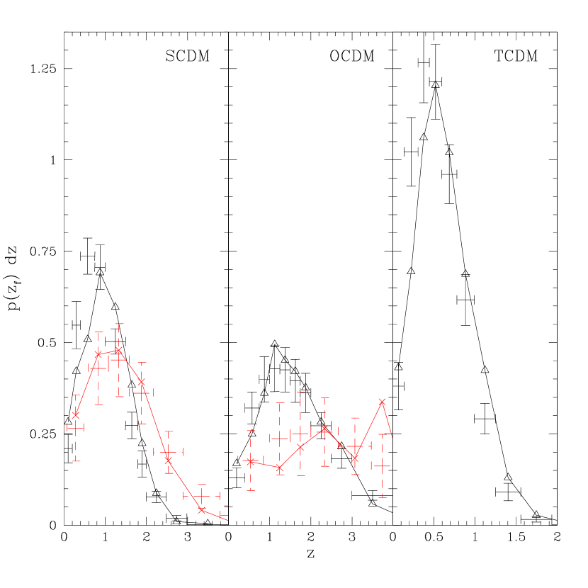
Figure 4: Probability distribution of formation redshift $p(z_{f})dz$ vs. redshift $z$. In each model, the solid line and triangular points represent the uniform volume, while the solid line and starred points denote the void simulations. The Monte-Carlo results are indicated by errorcrosses, with solid representing the uniform volumes and dashed representing the voids. The horizontal errorcross components denote the bin boundaries which were used for both the Monte-Carlo and simulated halos. The vertical components enclose 90% of 1000 bootstrap resamplings of the Monte-Carlo realizations. Thus, for EPS to match the simulated formation times the vertical errorbars must enclose 9 out of 10 points. Note that the horizontal scale for TCDM is half that of the other panels.

The difference in results can be examined more quantitatively by comparing halo formation times. A halo is said to have formed when the mass of the most massive progenitor is 50% of the z=0 mass. Given the discreteness of the simulation outputs, the formation time of simulated halos can only be bounded between adjacent outputs where the halo transitions the 50% formation threshold. Figure 4 plots the formation times of halos in simulations vs. their respective Monte-Carlo realizations. The points from the simulations (connected by lines) denote the number of halos formed in a bin $\Delta z$ where the bin boundaries correspond to simulation output times. In some cases multiple simulation outputs are combined into a single bin in order to increase statistics. In order to make a meaningful comparison, the formation time for each Monte-Carlo realization is binned in exactly the same manner as the simulation output. The bin boundaries are given by the horizontal bars in the Monte-Carlo data in Figure 4. To determine confidence limits, I bin 1000 bootstrap samples of the Monte-Carlo realization and show the regime in which 90% of the realizations fall as vertical errorbars. Consequently, for the simulation to match the EPS prediction, 90% of the simulation points should fall within the Monte-Carlo errorbars. As we expect from the mass history results, the EPS results are clearly different from SCDMu and TCDMu simulations at the 90% confidence level. The median formation time is a good measure for the “error” in formation time between simulated and EPS realizations. In SCDMu, the median simulated formation time in units of the $z=0$ age of an SCDM universe is approximately 0.20 while the Monte-Carlo realizations find a median formation time of 0.38. For OCDMu, 4 out of 10 simulated points are outside the errorbars, meaning that EPS also fails to match at the 90% confidence level. In the case of the void runs, the sampling errors are too large to rule out either Monte-Carlo realization, consistent with the interpretation from Figure 3. Consequently, the EPS appears to diverge notably from simulated realizations in flat models, as well as maintain a measurable difference in open models. The difference in the results between open and flat-matter cosmologies is most likely related to the growth of fluctuations in each. Since structure grows faster in $\Omega_{0}=1$ models, the differences between EPS and simulations is most likely exaggerated with respect to low-$\Omega_{0}$.

Note again that these results allow no freedom of choice of the critical density parameter $\delta_{c}$ as the PS and simulated mass functions are constrained to match at redshift $z=0$. Governato et al. (1999) provide evidence that a better fit can be attained by evolving $\delta_{c}$ in a nonlinear fashion. Hence, one is effectively renormalizing the mass function at every epoch, thus changing the mapping between perturbation spectrum and mass. If I use their fitting formula $\delta_{c}(z)=1.686\left[(0.7/\sigma_{8})(1+z)\right]^{-0.125}$ (valid for $\Omega_{0}=1$) for SCDMu, I find that this does indeed change the Monte-Carlo mass history of Figure 3b substantially. While the Monte-Carlo history is lower for small redshifts, it crosses the simulated curve and eventually diverges $2\sigma$ above the simulated histories for $z>1.4$. Governato et al. construct this relation from cluster-mass halos, well over an order of magnitude more massive than this study, so it is not surprising that using this fit does not induce EPS to match my simulated data. Still, the simulated results are bracketed with static $\delta_{c}$ producing too rapid halo growth and redshift-variant $\delta_{c}$ producing halos which grow slower than in N-body simulations. It may be possible to fine-tune a prescription for $\delta_{c}(z)$ to simulated data. As with any fine tuning of semi-analytic parameters, however, it is essential to understand the physical mechanisms underlying such parameters lest their predictive power be compromised. A study of such scope is best left to a future paper.

4 Conclusions

I present results from numerical N-body simulations regarding the effect of merging events on the angular momentum distribution of galactic halos as well as a comparison of halo growth in Monte-Carlo vs. N-body methods. In all three models tested and both in a uniform sample and in an underdense region, the distribution of halo spin parameters of merger remnants is greater than non-merger remnants. The spin parameters of the global halo population are consistent with other recent results Cole & Lacey (1996); Mo, Mao, & White (1998); Steinmetz & Bartelmann (1995); Catelan & Theuns (1996)). However, the K-S probabilities of merger and non-merger samples being from the same sample are quite low, and the mean spin parameters of the two samples $\bar{\lambda}$ are significantly different. The actual contribution of merging on the global spin parameter distribution depends on the fraction of halos that are merger-remnants and hence is greatly affected by cosmology. The overall effect of merging is to increase the mean and decrease the dispersion of the spin parameter distribution. I offer the tentative conclusion that this is consistent with the orbital angular momentum of the merging halos playing a major role in establishing the remnant’s resultant net angular momentum. The causes and time-evolution of this behavior should be investigated in greater detail in future studies using simulations of superior dynamic range. It is also possible that angular momentum distributions could vary as a function of redshift, but I leave this for a future paper.

I trace the most massive progenitor of halos of mass $M_{i}\sim 10^{13}M_{\odot}$ at redshift $z=0$ back to $z=5$ for “uniform volumes” in all three cosmologies as well as mass $M_{i}\sim 10^{11}M_{\odot}$ halos for large voids in the $\Omega_{0}=1$ and $\Omega_{0}=0.3$ cosmologies. I find that in the uniform volumes, the Press-Schechter based method reproduces the general trend of the simulated mass histories relatively well, although in $\Omega_{0}=1$ models it underpredicts the average mass history of halos by roughly 20%. This leads to a further discrepancy in the estimation of halo formation times. For example, the median formation time of halos in a flat universe (SCDMu) is 20% the age of the Universe according to simulations, but 38% the age of the Universe in Monte-Carlo realizations. Because the PS $z=0$ mass function is constrained to match the simulated halo mass function, $\delta_{c}$ is no longer a free parameter. It may be possible fine-tune PS to match simulated results by the use of a $\delta_{c}$ which evolves non-linearly with redshift, although such a study is beyond the scope of this paper.

My results are consistent with work by Somerville et al. (2000) and Tormen (1998). Somerville et al. find that EPS reproduces relative properties of the progenitor halo distribution, e.g. their mass ratios, quite well. However, the absolute progenitor masses and the overall conditional mass function exhibits discrepancies of up to 50%. Tormen concludes that the EPS formulation is inadequate to describe clustering in a constrained environment and may possibly be inadequate in a general context. I find that the latter is indeed true, as the conditional halo mass function in a cosmologically representative sample does not agree with simulated data. Consequently, care should be taken when comparing the raw masses of halo progenitors, or their mass relative to their eventual “children” of the present day. Formation times of halos from the EPS conditional mass function are systematically biased. Furthermore, care should be taken when examining the redshift evolution of any absolute quantity which depends on the evolution of mass, such luminosity or color. Halo properties should be compared in a relative sense at each redshift and not in an absolute sense with respect to their parents or children at other times.

Recently, alternative expressions for the PS mass function have been proposed and investigated. Sheth & Tormen (1999) modify the Press-Schechter formalism, producing a much better match to the mass function, especially at the low-mass end, of simulations. Mo, Sheth, & Tormen (1999) have shown that significant improvements to the standard PS approach can be made by modeling the formation of bound structures as an ellipsoidal rather than a spherical collapse. Jenkins et al. (2000) derive an empirical mass function by fitting the results numerous N-body simulations. My results further demonstrate the need for using these alternative approaches when generating Monte-Carlo mass histories.

References

- Abraham, et al. (1999) Abraham, R. G., Ellis, R. S., Fabian, A. C., Tanvir, N. R. and Glazebrook, K. 1999, MNRAS, 303, 641
- Bardeen et al. (1986) Bardeen, J., Bond, J.R., Kaiser, N. & Szalay, A.S. 1986, ApJ, 304, 15
- Barnes & Efstathiou (1987) Barnes, J.E., & Efstathiou, G. 1987, ApJ, 319, 575
- Baugh et al. (1998) Baugh, C.M., Cole, S., Frenk, C.S. & Lacey, C.G. 1998, ApJ, 498, 504
- Baugh et al. (1996) Baugh, C.M., Cole, S., & Frenk, C.S. 1996, MNRAS, 283, 1361
- Bertshinger (1985) Bertschinger, E. 1985 ApJS, 58, 39
- Bond et al. (1991) Bond, J.R., Cole, S., Efstathiou, G., & Kaiser, N., 1991, ApJ, 379, 440
- Borgani et al. (1999) Borgani, S. , Rosati, P. , Tozzi, P. & Norman, C. 1999, ApJ, 517, 40
- Bower (1991) Bower, R.J. 1991, MNRAS, 248, 332
- Bryan & Norman (1998) Bryan, G.L. & Norman, M.L. 1998, ApJ, 495, 80
- Catelan & Theuns (1996) Catelan, P. & Theuns, T. 1996, MNRAS, 282, 455
- Cavaliere, Menci, & Tozzi (1998) Cavaliere, A., Menci, N. & Tozzi, P. 1998, ApJ, 501, 493
- Cole & Lacey (1996) Cole, S. & Lacey, C. 1996, MNRAS, 281, 716
- Dalcanton, Spergel, & Summers (1997) Dalcanton, J.J., Spergel, D.N., & Summers, F.J. 1997, ApJ, 482, 659
- Davis et al. (1985) Davis, M., Efstathiou, G., Frenk, C.S., & White, S.D.M. 1985, ApJ, 292, 371
- de Carvalho & Djorgovski (1992) de Carvalho, R. R., & Djorgovski, S. 1992, ApJ, 389, 49
- Efstathiou et al. (1988) Efstathiou, G., Frenk, C.S., White, S.D.M. & Davis, M. 1988, MNRAS, 235, 715
- Frenk et al. (1988) Frenk, C.S., White, S.D. M., Davis, M. & Efstathiou, G. 1988, ApJ, 327, 507
- Gardner et al. (1997) Gardner, J.P., Katz, N., Hernquist, L., & Weinberg, D.H. 1997, ApJ, 484, 31.
- Gelb & Bertschinger (1994) Gelb, J.M. & Bertschinger, E. 1994, ApJ, 436, 467
- Ghigna et al. (1998) Ghigna, S. , Moore, B. , Governato, F. , Lake, G. , Quinn, T. & Stadel, J. 1998, MNRAS, 300, 146
- Governato et al. (1999) Governato, F., Babul, A., Quinn, T., Tozzi, P., Baugh, C.M., Katz, N. & Lake, G. 1999, MNRAS, 307, 949
- Governato et al. (1998) Governato, F., Gardner, J.P., Stadel, J., Quinn, T., & Lake, G. 1998, AJ, 117, 1651.
- Governato et al. (1997) Governato, F. , Moore, B. , Cen, R. , Stadel, J. , Lake, G. & Quinn, T. 1997, New Astronomy, 2, 91
- Governato & Tozzi (2001) Governato, F., & Tozzi, P. 2000, in preparation
- Grammann & Suhhonenko (1999) Grammann, M., & Suhhonenko, I. 1999, ApJ, 519, 433
- Gross et al. (1998) Gross, M.A.K., Somerville, R.S., Primack, J.R., Holtzman, J. & Klypin, A. 1998, MNRAS, 301, 81
- Huss, Jain, & Steinmetz (1999) Huss, A., Jain, B. & Steinmetz, M. 1999, MNRAS, 308, 1011
- Jenkins et al (2000) Jenkins, A., Frenk, C.S., White, S.D.M., Colberg, J.M., Cole, S., Evrard, A.E., Couchman, H.M.P., & Yoshida, N. 2000, MNRAS, submitted, Astro-ph/0005260
- Kaiser (1986) Kaiser, N. 1986, MNRAS, 222, 323
- Kauffmann (1996) Kauffmann, G. 1996, MNRAS, 281, 487
- Kauffmann (1995) Kauffmann, G. 1995, MNRAS, 274, 153
- (33) Kauffmann, G. & Charlot, S. 1998, MNRAS, 297, L23
- (34) Kauffmann, G. & Charlot, S. 1998, MNRAS, 294, 705
- Kauffmann & White (1993) Kauffmann, G., & White, S.D.M., 1993, MNRAS, 261, 921
- Kitayama & Suto (1996) Kitayama, T. & Suto, Y. 1996, ApJ, 469, 480
- Lacey & Cole (1994) Lacey, C., & Cole, S. 1994, MNRAS, 271, 676
- Lacey & Cole (1993) Lacey, C., & Cole, S. 1993, MNRAS, 262, 627
- Lemson & Kauffmann (1999) Lemson, G. & Kauffmann, G. 1999, MNRAS, 302, 111
- Levine & Sparke (1998) Levine, S. E., & Sparke, L. S. 1998, ApJ, 496, L13
- Longhetti et al. (1998) Longhetti, M., Rampazzo, R., Chiosi, C., & Bressan, A. 1998, A&AS, 130, 267
- Lupton (1993) Lupton, R. 1993, Statistics in Theory and Practice, pp. 126, Princeton
- Mo, Mao, & White (1998) Mo, H.J., Mao, S. & White, S.D.M. 1998, MNRAS, 295, 319
- Nagashima & Gouda (1998) Nagashima, M., & Gouda, N. 1998, MNRAS, 301, 849
- Governato & Tozzi (2000) Governato, F., & Tozzi, P. 2000, in preparation
- Peebles (1993) Peebles, P.J.E. 1993, Principles of Physical Cosmology, Princeton
- Press & Schechter (1974) Press, W.H., & Schechter, P. 1974, ApJ, 187, 425
- Richter & Sancisi (1994) Richter, O. & Sancisi, R. 1994, A&A, 290, L9
- Rose et al. (1994) Rose, J. A., Bower, R. G., Caldwell N., Ellis R. S., Sharples, R. M., & Teague, P. 1994, AJ, 108, 2054
- Rudnick & Rix (1998) Rudnick, F., & Rix, H. 1998, AJ, 116, 1163
- Rudnick, Rix, & Kennicut (2000) Rudnick, F., Rix, H., & Kennicutt, R.C. 2000, ApJ, in preparation
- Ryden (1998) Ryden, B.S. 1988, ApJ, 329, 589
- Schwarzkopf & Dettmar (2000) Schwarzkopf, U. & Dettmar, R. 2000, A&AS, 144, 85
- Sheth, Mo, & Tormen (1999) Sheth, R.K., Mo, H.J., & Tormen G. 1999, MNRAS, submitted, Astro-ph/9907024
- Sheth & Tormen (1999) Sheth, R.K. & Tormen, G. 1999, MNRAS, 308, 119
- Somerville et al. (2000) Somerville, R.S., Lemson, G., Kolatt, T.S., & Dekel, A. 2000, MNRAS, 316, 479
- Somerville & Primack (1999) Somerville, R.S. & Primack, J.R. 1999, MNRAS, 310, 1087
- Steinmetz & Bartelmann (1995) Steinmetz, M. & Bartelmann, M. 1995, MNRAS, 272, 570
- Tormen (1998) Tormen, G. 1998, MNRAS, 297, 648
- van den Bosch (1998) van den Bosch, F.C. 1998, ApJ, 507, 601
- Warren et al. (1992) Warren, M. S., Quinn, P.J., Salmon, J.K. & Zurek, W.H. 1992, ApJ, 399, 405
- White et al. (1993) White, S.D.M., Efstathiou, G., & Frenk, C.S. 1993, MNRAS, 262, 1023
- (63) Zaritsky, D. & Rix, H.-W. 1997, ApJ, 477, 118