The Far-Infrared emission of Radio Loud and Radio Quiet Quasars.

Abstract

Continuum observations at radio, millimetre, infrared and soft X-ray energies are presented for a sample of 22 quasars, consisting of flat and steep spectrum radio loud, radio intermediate and radio quiet objects. The primary observational distinctions, among the different kinds of quasars in the radio and IR energy domains are studied using large observational datasets provided by ISOPHOT on board the Infrared Space Observatory, by the IRAM interferometer, by the sub-millimetre array SCUBA on JCMT, and by the European Southern Observatory (ESO) facilities IRAC1 on the 2.2 m telescope and SEST.

The spectral energy distributions of all quasars from radio to IR energies are analyzed and modeled with non-thermal and thermal spectral components.

The dominant mechanism emitting in the far/mid-IR is thermal dust emission in all quasars, with the exception of flat spectrum radio loud quasars for which the presence of thermal IR emission remains rather uncertain, since it is difficult to separate it from the bright non-thermal component. The dust is predominantly heated by the optical/ultraviolet radiation emitted from the external components of the AGN. A starburst contributes to the IR emission at different levels, but always less than the AGN ($\leq$ 27%). The distribution of temperatures, sizes, masses, and luminosities of the emitting dust are independent of the quasar type.

1 Introduction

Radio quiet and radio loud (not blazar) quasars (RQQ and RLQ, respectively) have similar spectral properties in the ultraviolet (UV), optical, and infrared (IR), but their radio powers differ by several orders of magnitude (Elvis et al. (1994)). This divergence takes place at millimetre (mm) wavelengths. At these wavelengths the contribution from two emission components merge, namely the synchrotron emission dominant in the radio domain and thermal emission from cool dust (30-50 K) in the far-IR (Barvainis & Antonucci (1989)). It is still not entirely clear whether the distinction between RLQ and RQQ is a consequence of differences in their central engines or whether it merely reflects differences in their environments. The primary observational distinctions in the IR domain, and the proposed physical mechanisms to explain them are studied here, using the new insights provided by Infrared Space Observatory (ISO; Kessler et al. (1996)) measurements.

1.1 The Radio emission

Two main types of RLQ can be distinguished on the basis of their radio spectrum: the flat spectrum radio loud quasars (FSRQ), and the steep spectrum radio loud quasars (SSRQ). FSRQ show highly-collimated structures and very compact features, with flat or inverted radio spectra. SSRQ have radio spectra dominated by synchrotron emission from extended radio lobes. The lobes and a radio core in the centre of these objects are signs of a relativistic jet. According to the unified scheme (Barthel (1989); Urry & Padovani (1995)) FSRQ are the counterparts of SSRQ in which the jet is aimed at the observer.

The origin of the much weaker radio emission in RQQ is far less certain. The majority of the total radio emission from the RQQ comes from the compact features in the nucleus ($<$ 1 kpc for unresolved regions, and at least 2 kpc for the resolved ones) rather than the body of the host galaxy (Kukula et al. (1998)). It has been proposed that the activity in RQQ is supplied by a starburst, i.e. thermal bremsstrahlung and synchrotron emission coming from strongly radiative supernovæ  and supernovæ  remnants (SNRs) in a very dense environment where shocks accelerate electrons (Terlevich et al. (1992)). Alternatively, if the energy supply arises from accretion onto a massive black hole, the radio emission from RQQ (as in RLQ) is caused by radio jets, but the bulk kinetic power of these jets is for some reason $\sim$ 10³ times lower than those of RLQ (Miller et al. (1993)). This second hypothesis seems to be favored by recent studies, because of high brightness temperatures calculated (typical SN/SNRs have T${}_{\mathrm{B}}\leq 10^{5}$K), by the evidence of a pc-scale jet (Blundell & Beasley (1998)) and by observations of flat/inverted and variable radio spectra (Barvainis et al. (1996)).

Recently, quasars with intermediate radio luminosities have been discovered and labeled Radio Intermediate Quasars (RIQ) (Francis et al. (1993), Falcke et al. (1995)). RIQ may represent the Doppler boosted counterparts of radio quiet quasars. This hypothesis is suggested by the variability observed at radio wavelengths (Falcke et al. (1996)).

1.2 The Infrared emission

The presence of a dominant thermal (circumnuclear dust emission), or non-thermal (synchrotron radiation from the AGN) component in the IR continuum of quasars is still debated.

Many attempts to establish the origin of the IR emission in RLQ and RQQ have been performed through observations in the sub-millimetre (sub-mm) of quasars detected by IRAS (RLQ in Chini et al. 1989a , and Antonucci et al. (1990); RQQ in Chini et al. 1989b , Barvainis et al. (1992), Hughes et al. (1993), and Hughes et al. (1997); and both in Andreani et al. (1999), this last work is the only one based on an optically selected sample). The main test applied to recognize the presence of thermal emission in the IR spectra of the objects was based on the slope of the continuum emission (F${}_{\nu}\propto\nu^{\alpha}$) connecting the far-IR and sub-mm data. A steep, $\alpha\,>$ 2.5, continuum is strong evidence for thermal dust emission. Most of the sources studied have $\alpha\,<$ 2.5 and are consistent with a dominant self-absorbed synchrotron emission component. However, some RQQ have spectral slopes as steep as $\alpha$ = 4.35, which, along with observations of strong molecular gas (CO) emission (Barvainis (1997)), give strong support to a thermal mechanism as the origin of the far-IR component in RQQ.

Among the RLQ, $\alpha$ is, at most, $\simeq$ 0.9 for the FSRQ, and 1.1 for the SSRQ (Chini et al. 1989a ). Variability, shape of the continuum spectral energy distribution and, in some cases polarization, indicate that the radio, mm and far-IR emission of FSRQ is dominated by the synchrotron process (Lawrence et al. (1991)). On the contrary, many SSRQ show evidence of thermal emission: their far-IR spectra are brighter than extensions of the radio emission (Antonucci et al. (1990)), suggesting a different origin than the non-thermal radio component; and the flux is constant, consistent with it arising from a region much larger than a light year (Edelson & Malkan (1987)). Moreover, the spectral energy distributions of some RLQ, both FSRQ and SSRQ, show evidence for a galaxy component: reddening, residual starlight, molecular gas (Scoville et al. (1993)), and some thermal dust emission in the near-IR (Barvainis (1987)). Both components, non-thermal synchrotron radiation and thermal dust emission, are probably present at IR wavelengths, as observed in the RLQ 3C273 (Robson et al. (1986); Barvainis (1987)).

1.3 Relation between the Radio and Infrared emission

A tight, linear correlation is observed between the far-IR flux and the radio fluxes in AGN (Sopp & Alexander (1991)), suggesting a common origin. RQQ and RLQ occupy well defined regions in Log($L$(IR))–Log($L$(Radio)) space, and show a relation with a similar slope, just shifted to higher radio power by a factor $\sim$10⁴ in RLQ. RQQ show a similar relation as spirals, starbursts, and ultra luminous IR galaxies (ULIRG), suggesting that their IR emission may arise from sufficiently energetic star formation in the host galaxy (Sopp & Alexander (1991)). However, the majority of the bolometric luminosity in over half of known ULIRG seems to arise from a buried AGN (Sanders (1999)). Additionally, the variable and flat spectra, and high brightness temperatures shown by many RQQ at radio frequencies (Barvainis et al. (1996)) suggest that the radio emission is related to the AGN rather than to a starburst.

1.4 Proposed scenarios

The unified model (Barthel (1989); Urry & Padovani (1995)) predicts that similar disk–like dust distributions exist in both RQQ and RLQ. Orientation of the active nucleus, environment, and jet luminosity all affect the relative contributions of thermal and non-thermal sources to the observed infrared luminosity (Chini et al. 1989a ).

Other scenarios have been proposed to explain the large differences in radio power between RQQ and RLQ: different spin of the central black hole (Wilson & Colbert (1995)), or different morphological type of the host galaxy. Indeed, different radio powers are expected if one population of objects is fueled by mergers (ellipticals) and one is fueled by mostly internal processes within the galaxy (spirals) (Wilson & Colbert (1995)). However, recent studies on the host galaxies of quasars indicate that the host galaxies of RQQ are in several cases elliptical and not always spiral galaxies (Taylor et al. (1996)).

1.5 Open issues

A better knowledge of the radio and IR properties of quasars is required to test the unified model predictions, and answer the following questions:

1. What is the dominant mechanism emitting at IR wavelengths in RLQ and RQQ?

2. Do RLQ and RQQ have the same dust properties (temperature, source size, mass, and luminosity)?

3. Does an interplay between the radio and the IR components exist?

These questions can be addressed through the study of the spectral energy distributions (SED) of RLQ and RQQ. Here, we present the SEDs from radio to IR frequencies of a sample of 22 AGN (7 RQQ, 11 RLQ, 2 radio galaxies (RG) and 2 RIQ). The selected sample, even if incomplete and heterogeneous, is useful to address these questions thanks to several properties characterizing the sample (steep/flat radio spectra, radio loudness/quietness), and to the large amount of photometric data available in the radio, mm/sub-mm and IR domains. This work is based mainly on IR data provided by ISO. ISO data reduce the frequency gap between sub-mm and far-IR observations, better sample the IR spectral band with a larger number of filters than previous instruments, and increase the number of detected objects thanks to a higher sensitivity. The study of the IR emission of quasars will be extended in the future with the results of the European and of the U.S. ISO Key Quasar Programs providing a similar coverage of the IR SED for a larger sample of quasars (see first results in Haas et al. (1998), and Wilkes et al. (1999)).

2 Observational dataset

Source names, coordinates, and redshifts of the selected sample were taken from the NASA Extragalactic Database (NED), and are listed in Table 1. Infrared observations were obtained for 18 of the sources with the Imaging Photopolarimeter on ISO (ISOPHOT; Lemke et al. (1996)), and 3 were observed with IRAC1 on the 2.2 m ESO/MPE telescope. Millimetre and sub-mm data were obtained for 10 objects with the IRAM interferometer at Plateau de Bure in France (Guilloteau et al. (1992)), the Sub-millimetre Common User Bolometer Array (SCUBA; Holland et al. (1999)) on the James Clerk Maxwell Telescope and the Swedish ESO Sub-mm Telescope (SEST) of the European Southern Observatory (ESO) at La Silla. The instruments used for each object are indicated in a footnote to Table 1.

Table 1: Basic properties of the sample

Source	RA (J2000)	Dec (J2000)	Type†	z
Name	$h\;\;m\;\;s$	$\degr\;\;\arcmin\;\;\arcsec$
3C 471,4	01 36 24	+20 57 27	SSRQ	0.425
PKS 0135$-$2471	01 37 38	$-$24 30 53	FSRQ	0.831
PKS 0408$-$651,2	04 08 20	$-$65 45 09	RG	…
PKS 0637$-$751,2	06 35 47	$-$75 16 17	FSRQ	0.653
PG 1004+1302	10 07 26	+12 48 56	SSRQ	0.240
PG 1048$-$0902	10 51 30	$-$09 18 10	SSRQ	0.344
4C 61.201	10 52 33	+61 35 20	SSRQ	0.422
PG 1100+7721,5	11 04 14	+76 58 58	SSRQ	0.312
PG 1103$-$0062	11 06 32	$-$00 52 52	SSRQ	0.423
PG 1216+0691,2	12 19 21	+06 38 38	RIQa	0.331
PG 1352+1831	13 54 36	+18 05 18	RQQ	0.152
PG 1354+2131	13 56 33	+21 03 51	RQQ	0.300
PG 1435$-$0671,3	14 38 16	$-$06 58 21	RQQ	0.129
PG 1519+2261	15 21 14	+22 27 43	RQQ	0.137
PG 1543+4891,5	15 45 30	+48 46 09	RQQ	0.400
PG 1718+4811	17 19 38	+48 04 13	RIQa	1.084
B2 1721+341	17 23 20	+34 17 58	SSRQ	0.206
HS 1946+76581,4	19 44 55	+77 05 52	RQQ	3.020
3C 4051	19 59 28	+40 44 01	NLRG	0.056
B2 2201+31A1	22 03 15	+31 45 38	FSRQ	0.295
PG 2214+1393	22 17 12	+14 14 21	RQQ	0.066
PG 2308+0981,3	23 11 18	+10 08 15	SSRQ	0.433

^† SSRQ: Steep Spectrum Radio Loud Quasar; FSRQ: Flat Spectrum Radio Loud Quasar; RQQ: Radio Loud Quasar; RIQ: Radio Intermediate Quasar; NLRG: Narrow Line Radio Galaxy; RG: Radio Galaxy.

¹ Observed with ISOPHOT; ² Observed with SEST; ³ Observed with IRAC1; ⁴ Observed with IRAM; ⁵ Observed with SCUBA.

^a Classification in Falcke et al. (1996).

The observational details (observing date, wavelength, and measured flux density) of IRAC1, SEST, IRAM, and SCUBA observations are reported in Table 2. The data obtained with the SEST telescope were reduced to outside the atmosphere, corrected for the gain elevation characteristic of the telescope, and calibrated with Uranus. All IRAM observations were performed in compact configuration. All five antenna were used during most of the observations, with the exceptions indicated in a footnote of Table 2. The calibrators were 3C 454.3 for 3C 47, and 22040+420 and 1928+738 during the two observations of HS 1946+7658. SCUBA observations yielded good results at 850 $\mu$m only due to marginal weather. The fluxes were calibrated using the canonical gain value of 220 Jy/V, since a calibration scan at 850$\mu$m was not done. The chosen value is relatively insensitive to the weather and should be good to within 20%. ISOPHOT observations and data reduction are described in the next section. These new observations were supplemented with literature data from radio to near-IR. We have also collected data at soft X-ray energies. For reasons of homogeneity we collected only ROSAT data, available for most of the sources. From published soft X-ray spectra we derived the flux at 1 keV corrected for absorption. The observed absorption is always compatible with the galactic absorption. The list of references from which data were retrieved, for each object, is reported in Table 3.

Table 2: IRAC1, SEST, IRAM and SCUBA results

Source Name	Instrum.	Obs. Date	$\lambda$	F${}_{\nu}^{\dagger}\;\;\;\;$
		($d\;m\;y$)	($\mu$m)	(mJy)
3C 47	IRAM	14 07 981,2	1300	17.0$\pm$2.3
		14 07 981,3	3000	30.8$\pm$0.6
PKS 0408$-$65	SEST	30 11 95	1300	$<$30
PKS 0637$-$752	SEST	30 11 95	1300	724$\pm$37
			1300	905$\pm$31
PG 1004+130	SEST	30 11 95	1300	$<$39
PG 1048$-$090	SEST	30 11 95	1300	$<$18
PG 1100+772	SCUBA	17 01 99	850	6.8$\pm$2.4
PG 1103$-$006	SEST	30 11 95	1300	$<$27
PG 1216+069	SEST	30 11 95	1300	$<$45
PG 1435$-$067	IRAC1	21 06 96	3.7	12.1$\pm$0.4
			3.7	12.2$\pm$0.5
PG 1543+489	SCUBA	17 01 99	850	$<$5.4
HS 1946+7658	IRAM	20 05 984	1300	$<$10.4
		20 05 984	3000	$<$5.0
PG 2214+139	IRAC1	21 06 96	4.7	44.2$\pm$4.6
PG 2308+098	IRAC1	21 06 96	3.7	$<$17.56

^† Upper limits to the flux are given at the 3$\sigma$ level. ¹ Also observed on July 17, and 22. ² Only four antenna were used on July 17. ³ Only three antenna were used on July 14, and four on July 17, and 22. ⁴ Also observed on May 23.

Table 3: List of references of selected published data

Source Name		References number†
3C 47		1, 2, 3, 4, 5
PKS 0135$-$247		1, 3, 5, 6, 7
PKS 0408$-$65		1
PKS 0637$-$75		1, 2, 3, 5, 6, 8, 9
PG 1004+130		1, 10, 11, 12, 13, 14, 15, 16
PG 1048$-$090		1, 3, 11, 14, 15, 17
4C 61.20		1, 3, 18
PG 1100+772		1, 2, 3, 12, 15, 17, 19, 20, 21
PG 1103$-$006		1, 12, 14, 15, 22, 23
PG 1216+069		2, 12, 14, 23, 24, 25, 26
PG 1352+183		2, 14, 15, 17, 25
PG 1354+213		2, 14, 15, 25
PG 1435$-$067		2, 14, 15, 25
PG 1519+226		2, 14, 15, 25
PG 1543+489		12, 14, 15, 25, 27, 28, 29
PG 1718+481		1, 2, 14, 23, 26, 30
B2 1721+34		1, 13, 17, 31
HS 1946+7658		25, 32
3C 405		1, 33, 34
B2 2201+31A		1, 2, 7, 13, 16, 20, 31, 35, 36, 37
		38, 39, 40, 41
PG 2214+139		1, 12, 15, 29, 30, 42
PG 2308+098		1, 15, 30

† 1: NED; 2: Gezari et al. (1997);	3: Brinkmann et al. (1997);
4: van Bemmel et al. (1998);	5: Kühr et al. (1981);
6: Tornikoski et al. (1996);	7: Steppe et al. (1993);
8: Véron-Cetty & Véron (1998);	9: Tanner et al. (1996);
10: Wilkes et al. (1994);	11: Kapahi (1995);
12: Sanders et al. (1989);	13: Lister et al. (1994);
14: Neugebauer et al. (1987);	15: Miller et al. (1993);
16: Ennis et al. (1982);	17: Elvis et al. (1994);
18: Reid et al. (1995);	19: Antonucci et al. (1990);
20: Chini et al. 1989a ;	21: Lonsdale & Morison (1983);
22: Siebert et al. (1998);	23: Kellermann et al. (1989);
24: Blundell & Beasley (1998);	25: Yuan et al. (1998);
26: Falcke et al. (1996);	27: Andreani et al. (1999);
28: Barvainis et al. (1996);	29: Chini et al. 1989b ;
30: Wang et al. (1996);	31: Schartel et al. (1996);
32: Kuhn et al. (1995);	33: Robson et al. (1998);
34: Haas et al. (1998);	35: Bloom et al. (1999);
36: Hoekstra et al. (1997);	37: Mitchell et al. (1994);
38: Neugebauer et al. (1986);	39: Ghosh et al. (1994);
40: Neugebauer et al. (1979);	41: Teräsranta et al. (1992);
42: Hughes et al. (1993).

3 ISOPHOT observations and data reduction

Photometric data at several (up to 11) wavelengths between 3.6 and 200 $\mu$m were obtained for each object using the single-element P1 and P2 detectors plus the two array cameras, C100 (3 pixels $\times$ 3 pixels) and C200 (2 pixels $\times$ 2 pixels). Detector and observing parameters are listed in Table 4. Most of the observations (124 in total for 16 objects) were performed in chopper mode, and the remaining (37 for 10 objects) by mapping the region surrounding the target (scans or rasters).

Table 4: ISOPHOT detector properties and covered sky region in mapping observations

Detector	$\lambda$	Pixel	Scan	Raster
Name	( $\mu$m )	size	Coverage
		( $\arcsec$ )	( $\arcsec\times\arcsec$ )	( $\arcsec\times\arcsec$ )
P1	3.6, 4.8, 7.3, 12	-	52$\times$156	-
P2	25	-	-	-
C100	60, 80, 100	43.5	138$\times$230	230$\times$230
C200	150, 170, 200	89.4	184$\times$460	276$\times$460

In chopper mode the radiation beam is deflected from the source (on-source position) to adjacent fields on the sky (off-source position) several times in order to measure the background emission. Triangular (T) and rectangular (R) chopping modes were used. In the triangular chopper mode the background emission is measured in two different regions, while in the rectangular chopper mode it is measured in only one position. Observing dates, filters, apertures, exposure times, chopping mode, and measured fluxes are reported in Table 5 for each ISOPHOT chopper observations.

In mapping mode the telescope moves in a pattern around the source, providing more sky coverage than in the chopper mode (Table 4). P1 detector maps were performed with an aperture of 52$\arcsec$ during all observations, except one (B2 2201+31A) during which the chosen aperture was 23$\arcsec$. Observing dates, filters, exposure times, and measured fluxes are reported in Table 6. More details on mapping mode are reported in section 3.2.1.

3.1 First steps of the data reduction: from ERD to AAP level

The first part of the data reduction was performed using version 8.1 of the PHT Interactive Analysis (PIA) tool (Gabriel (1997)). We started the reduction with the raw data processed with version 8.7 of the Off-Line Processing (Laureijs et al. (1998)). The raw data form a sequence of detector read-outs distributed in 2ⁿ ($n$=2-6) sets of four response curves or ramps, as function of time (Edited Raw Data: ERD in Volts).

Each set of four ramps represents a sky position. Each ramp is corrected for the non-linearity of the detector response, and for contamination of cosmic particle events (glitches). The removal of read-outs affected by glitches is carried out by applying two median filtering techniques: the single-threshold technique that uses a threshold of 4.5 standard deviations ($\sigma$) for flagging bad read-outs and the two-threshold technique that uses a threshold of 3.0$\sigma$ for flagging and 1.0$\sigma$ for re-accepting read-outs. After applying the non-linearity correction and the deglitching to the ERD, a straight line is fitted to each ramp, in order to determine its slope or Signal per Ramp Data (SRD in Volt/s).

In most of the cases the first 25 or 50% (1 or 2 ramps of 4) of the signals per chopper plateau at the SRD level are discarded to enable the detector response to stabilize at the level corresponding to the source flux density. The remaining data are further corrected for highly discrepant points (value at more than 3$\sigma$ from the average signal) still contaminated by glitches, for the orbital dependent dark current, and for the signal dependence on the ramp integration time (reset time interval) to obtain an average Signal per Chopper Plateau (SCP in Volt/s).

After applying flat-fielding correction using PIA values, the SCP data are calibrated to obtain the Standard Processed Data (SPD in unit of Watts). Since the detector response varies with time, it is determined at the time of the observation by measuring the flux emitted by two thermal Fine Calibration Sources (FCS1 and FCS2) on board. The FCS measurements are reduced in the same way as the scientific measurements up to this step. Data from FCS1 are used because they are the best calibrated. The FCS1 signal is checked in order to remove data with large uncertainties (this step is equivalent to computing the weighted mean of the FCS1 data).

In the case of mapping observations, the FCS1 is observed twice, before and after the observation of the source. The photometric calibration we use is the average value of the two FCS1 measurements.

After the flux calibration the AAP (Auto Analysis Product) data are obtained. They are a sequence of 2ⁿ off- and on-source flux measurements (in Jy) each corresponding to a sky position. The reduction from the AAP level to the final results is performed using our own IDL routines, and not following the standard pipeline. This procedure was also applied in the reduction of ISOPHOT chopper data of a sample of Seyfert galaxies (Polletta & Courvoisier (1999)).

Table 5: Details of ISOPHOT Observations performed in Chopper Mode

$\lambda$	Apt.	Exp.	Chop.	Fν	Uncert.†
($\mu$m)	($\arcsec$)	(s)	Mode	(mJy)	Stat.	Syst.
3C 47 (January 30, 1997)
4.8	23	128	R	$<$64.
12.8	23	128	R	69.	10.	21.
20	23	128	R	$<$171.
60	-	256	R	170.	52.	51.
100	-	256	R	246.	52.	74.
PKS 0408$-$65 (June, 05 1997)
4.8	23	128	R	$<$26.
12.8	23	128	R	$<$60.
20	23	128	R	$<$84.
60	-	128	R	$<$308.
100	-	128	R	$<$162.
PKS 0637$-$75 (June, 05 1997)
4.8	23	128	R	$<$26.
12.8	23	128	R	$<$43.
20	23	128	R	$<$99.
60	-	128	R	$<$117.
100	-	128	R	$<$143.
4C 61.20 (April, 27 1996)
7.3	13.8	512	T	$<$35.
12	23	256	T	$<$34.
25	52	512	T	$<$110.
60	-	128	R	$<$278.
80	-	128	R	258.	48.	77.
100	-	128	R	$<$303.
150	-	128	R	$<$267.
170	-	128	R	$<$148.
200	-	128	R	$<$335.

• In units of mJy.

Table 5: (continued)

$\lambda$	Apt.	Exp.	Chop.	Fν	Uncert.†
($\mu$m)	($\arcsec$)	(s)	Mode	(mJy)	Stat.	Syst.
PG 1100+772 (June, 17 1996)
4.8	52	512	R	25.	7.	8.
7.3	52	512	R	32.	5.	10.
12	52	512	R	36.	8.	11.
25	120	512	R	54.	10.	16.
60	-	256	R	70.	14.	21.
100	-	128	R	$<$282.
150	-	512	R	$<$417.
200	-	512	R	$<$468.
PG 1216+069 (July, 11 1996)
4.8	52	512	R	50.	15.	15.
7.3	52	512	R	72.	6.	22.
12	52	512	R	90.	12.	27.
25	120	512	R	95.	26.	29.
60	-	128	R	65.	14.	20.
100	-	128	R	$<$140.
150	-	512	R	$<$137.
200	-	512	R	$<$149.
PG 1352+183 (December, 14 1996)
60	-	64	R	198.	23.	59.
80	-	64	R	$<$237.
100	-	64	R	$<$213.
150	-	64	R	$<$283.
170	-	64	R	$<$240.
200	-	64	R	$<$206.
PG 1354+213 (June, 13 1996)
7.3	13.8	2048	T	18.	5.	5.
12	23	1024	T	21.	5.	6.
25	52	2048	T	23.	7.	7.
60	-	128	R	$<$298.
80	-	128	R	$<$194.
100	-	128	R	$<$125.
150	-	128	R	$<$170.
170	-	128	R	$<$137.
200	-	128	R	$<$280.

• In units of mJy.

Table 5: (continued)

$\lambda$	Apt.	Exp.	Chop.	Fν	Uncert.†
($\mu$m)	($\arcsec$)	(s)	Mode	(mJy)	Stat.	Syst.
PG 1435$-$067 (January, 07 1997)
7.3	13.8	256	T	70.	9.	21.
12	23	64	T	$<$94.
25	52	128	T	$<$718.
60	-	64	R	$<$1111.
80	-	64	R	$<$849.
100	-	64	R	$<$333.
150	-	64	R	$<$386.
170	-	64	R	$<$369.
200	-	64	R	$<$317.
PG 1519+226 (February, 01 1997)
7.3	13.8	256	T	32.	8.	10.
12	23	64	T	$<$48.
25	52	64	T	76.	17.	23.
60	-	128	R	172.	44.	52.
80	-	128	R	$<$194.
100	-	128	R	121.	22.	36.
150	-	128	R	$<$207.
170	-	128	R	$<$151.
200	-	128	R	$<$154.
PG 1543+489 (May, 30 1996)
4.8	52	512	R	20.	6.	6.
7.3	52	256	R	39.	4.	12.
12	52	256	R	45.	6.	14.
25	120	512	R	140.	13.	42.
60	-	128	R	470.	144.	141.
100	-	128	R	399.	55.	120.
150	-	128	R	455.	117.	182.
200	-	256	R	$<$377.
PG 1718+481 (May, 30 1996)
4.8	52	512	R	18.	3.	5.
7.3	52	256	R	24.	6.	7.
12	52	256	R	25.	6.	8.
25	120	512	R	44.	7.	13.
60	-	128	R	90.	1.	27.
100	-	128	R	56.	1.	17.
150	-	128	R	$<$251.
200	-	256	R	$<$261.

• In units of mJy.

Table 5: (continued)

$\lambda$	Apt.	Exp.	Chop.	Fν	Uncert.†
($\mu$m)	($\arcsec$)	(s)	Mode	(mJy)	Stat.	Syst.
B2 1721+34 (April, 20 1996)
7.3	13.8	512	T	19.‡	5.	6.
12	23	512	T	$<$26.‡
25	52	512	T	$<$135.‡
HS 1946+7658 (May, 27 1996)
4.8	52	1024	R	$<$5.
7.3	52	1024	R	4.5	1.2	1.4
12	52	1024	R	8.7	0.7	2.6
25	120	1024	R	47.	15.	14.
60	-	64	R	$<$230.
100	-	64	R	$<$300.
150	-	64	R	682.‡	17.	273.
200	-	64	R	378.‡	27.	151.
B2 2201+31A (November, 16 1996)
3.6	5	2048	T	$<$17.
4.8	7.6	1024	T	$<$52.
7.3	13.8	256	T	45.	5.	14.
12	23	64	T	64.	8.	19.
12	23	64	T	$<$62.
25	52	128	T	106.	25.	32.
60	-	128	R	193.	13.	58.
80	-	128	R	139.	11.	42.
100	-	128	R	212.	51.	64.
150	-	128	R	847.	97.	339.
170	-	128	R	699.	98.	280.
200	-	128	R	382.	97.	153.
PG 2308+098 (November, 26 1996)
3.6	5	2048	T	$<$31.
4.8	7.6	1024	T	13.	2.	4.
12	23	128	T	$<$39.
PG 2308+098 (December, 12 1996)
7.3	13.8	256	T	$<$21.
12	23	128	T	16.	55.	5.
25	52	512	T	$<$108.
60	-	128	R	$<$183.
80	-	128	R	$<$174.
100	-	128	R	$<$83.
150	-	128	R	$<$201.
170	-	128	R	$<$152.
200	-	128	R	$<$214.

^† In units of mJy. ^‡ Doubtful data. Discussed in Sec. 3.3 and 4.1.

Table 6: Details of ISOPHOT Observations performed in Raster Mode

Obs. date	$\lambda$	Exp.	Fν	Uncert.†
	($\mu$m)	(s)	(mJy)	Stat.	Syst.
3C 47
January, 31 1998	60	636	$<$129.
PKS 0135$-$247
December, 12 1997	12d	1206	$<$199.
PKS 0408$-$65
June, 05 1997	170a	195	$<$51.
PKS 0637$-$75
June, 05 1997	170a	346	$<$180.
March, 15 1998	150a	387	$<$171.
	200a	387	$<$203.
PG 1100+772
August, 15 1997	60	348	$<$99.
	100	348	$<$55.
	150b,c	579	$<$82.
	200b,c	579	$<$54.
October, 28 1997	12d	954	$<$161.
	60d	630	68.	22.	20.
November, 02 1997	150a	579	$<$120.
PG 1543+489
November, 01 1997	12d	864	$<$202.
	60d	630	269.	27.	81.
	150a,d	574	279.	45.	84.

^† In units of mJy. ^a4$\times$2 map. ^b2$\times$4 map. ^cStep amplitude of 90$\arcsec$. ^dTelescope nodding mode.

Table 6: (continued)

Obs. date	$\lambda$	Exp.	Fν	Uncert.†
	($\mu$m)	(s)	(mJy)	Stat.	Syst.
PG 1718+481
April, 20 1997	60	348	59.	16.	18.
	100	348	40.	13.	12.
	150a	323	$<$104.
	200a	579	$<$56.
November, 01 1997	12d	864	$<$164.
	60d	630	69.	13.	21.
	150a,d	574	$<$145.
HS 1946+7658
April, 28 1997	60	348	49.	12.	15.
	100	348	79.	14.	24.
	150a	451	$<$114.
	200a	579	$<$356.
October, 26 1997	200a	579	$<$227.
November, 17 1997	12d	954	$<$171.
November, 18 1997	12d	954	$<$168.
	60d	630	66.	15.	20.
December, 08 1997	60d	630	68.	20.	20.
3C 405
October, 30 1997	60d	630	2360.	76.	708.
	170a,d	574	1582.	160.	475.
B2 2201+31A
November, 20 1997	12d	852	55.	15.	17.
	60d	414	111.	20.	33.
	170a	387	$<$249.

^† In units of mJy. ^a4$\times$2 map. ^b2$\times$4 map. ^cStep amplitude of 90$\arcsec$. ^dTelescope nodding mode.

3.2 From the AAP level to final results

The last steps of the data reduction before determining the source flux are the background subtraction, the deletion of remaining highly discrepant points, and the correction for effects depending on chopper plateau time, vignetting (only for chopper observations) and point spread function.

In the case of chopper observations with the C100 detector only the central pixel pointed on the source is considered to derive the flux density, since the eight border pixels contain only a small fraction of the central point source and summing these values would hence only increase the noise.

3.2.1 Background subtraction

In chopper observations the background is measured at each off-source position. Since in some cases the instruments show long term drift effects, the background signal is estimated near the time of each on-source measurement and subtracted. In the case of chopper observations the background estimates are obtained by computing the weighted mean of each pair of consecutive off-source measurements. The weights are computed from PIA statistical uncertainties. Since the sequence of chopper plateaux ends with an on-source position, we used the weighted mean of the two last on-source measurements, and the flux observed in the last off-source position to determine the last pair of on- and off-source values, for a total of 2^n-1 flux values.

Small maps of the regions immediately surrounding ten of the targets were constructed in one or both of the following ways (Fig. 1): multiple linear scans across the source and rastering the detector about the source. A scan with the P1 and C100 detectors consisted of three steps of the telescope, with this sequence repeated three times. Only the middle row of C100 pixels (8, 5, and 2, as depicted in Fig. 1) viewed the source. The C200 scans contained four steps, repeated twice, with the source centered between two pixels. Note that the source was observed in only the middle two steps of the C200 scan. The raster patterns were 3$\times$3, 3$\times$3, and 4$\times$2 or 2$\times$4, for the P1, C100, and C200 detectors, respectively. Each pixel viewed the source once in the raster maps. The step size between exposures for both scans and rasters was approximately equal to the pixel size, a little more to take into account the gap between pixels, for the C100 and C200 cameras, and equal to the aperture size for the P1 detectors, which resulted in a different total sky coverage for each detector (see Table 4). A background estimate for each on-source measurement was obtained from a weighted average of the flux measured in the raster or scan positions immediately preceding and following the source position by the same pixel. Using the same pixel to determine the background reduced the impact of uncertainties in the flat field. The weighted average background was subtracted from each on-source measurement providing a sequence of source flux values.

Figure 1: Schematic representation of the two observing modes used for mapping observations: telescope nodding (scan) on the left side and classical raster on the right side. The position of the source in the different cases is represented by a star. The bold square represents the initial position of the detector. The numbering corresponds to the pixels numbers. The detectors move first from the left to the right, then in the opposite direction. In the case of classical raster, at each change of the horizontal direction, the detector shifts down one step. All the steps are separated by the pixel size. The reported pixel sizes do not correspond to the real proportions. The numbers in parenthesis refer to the number of horizontal steps $\times$ the number of repetitions for nodding and vertical steps of telescope motion in the raster maps.

Residual effects of detector instabilities, in both chopper observations and maps, produced occasional discrepant points, which were culled by one-pass sigma clipping. The threshold number of standard deviations to reject a flux value depended on the number of points in the sequence (Chauvenet’s criterion in Taylor (1982)), ranging from 1.15$\sigma$ to 2.66$\sigma$.

In the case of chopper observations with the C200 camera, the source flux was computed by adding together the fluxes measured by each of the four pixels. The source flux was divided between pairs of adjoining pixels in the C200 scans; these were averaged by weighting with their uncertainties. Table 6 lists the weighted mean of each flux sequence after clipping, or 3$\sigma$ upper limits for non–detection, where $\sigma$ is the quadratic sum of the statistical and systematic uncertainties (see section 3.3), also reported in the tables.

3.2.2 Vignetting correction

In the case of chopper observations with the C100 and C200 detectors, the data are further corrected for the signal loss outside the beam of the telescope (vignetting). The PIA default vignetting correction factors were computed considering the dependency only on the distance of the chopper positions and on the filter, but recent investigations have shown that they depend also on the time per chopper plateau (M. Haas, private communication).

The PIA default vignetting factors were applied directly to the data, resulting in little change to the flux values obtained with the C100 camera. However, the fluxes from the C200 detector are $\sim$ 80%, in median, larger after the vignetting correction. Given the uncertainty over the accuracy of the vignetting factors, we averaged the fluxes derived with and without the correction and added the respective uncertainties in quadrature.

3.2.3 Correction for effects depending on the chopper plateau time and point spread function

In the case of chopper observations a correction for the signal loss due to effects depending on the time per chopper plateau is applied to the computed flux value. Since short integration times with the C100 and C200 detectors do not reach the full signal, the observed flux can be reduced by large factors, typically up to 68 % for the C100 detector, and up to 12% for the C200 detector for the shortest observations. The correction factors we use are the PIA default values.

All the computed fluxes are finally corrected for the point spread function (psf) of each detector using the default PIA values derived empirically in most of the cases. The available psf correction values correspond to a source position centered in a pixel or located in a corner of the pixel. In case of scans with the C200 detector we needed the psf correction corresponding to the target located in the middle of a side of the pixel. We derived it by assuming a bi-dimensional Gaussian function for the psf and constraining its parameters using the other two known values for each wavelength (30.6% at 150 $\mu$m, and 29.1% at 170 $\mu$m).

3.3 Calculation of systematic uncertainties

During the data reduction only statistical errors were taken into account, and not those in the absolute flux density calibration. The accuracy of the absolute photometric calibration depends mainly on systematic errors (detector transient effects, calibration response, dark current, point spread function), and it is currently known to be better than 30% (Klaas et al. (1998)). The associated statistical and systematic uncertainties are reported in the last two columns of Table 5 and 6. We associate to the measured flux an uncertainty that is the quadratic sum of their statistical uncertainties and 30% (for the C200 measurements obtained in chopper mode we use 40% that corresponds to half of the uncertainty due to the vignetting correction) of the measured value. Among our ISOPHOT observations the datasets of B2 1721+34 were identified as failed after inspection of their quality by the ISO team because they were heavily affected by cosmic rays and thus scientifically useless. We report these data in Table 5, and indicate that they are doubtful in a footnote.

4 The spectral energy distributions

We report the first far-IR detection for 9 (4C 61.20, PG 1216+069, PG 1352+183, PG 1354+213, PG 1435$-$067, PG 1519+226, PG 1718+481, PG 2308+098, and HS 1946+7658) of the 18 sources observed with ISOPHOT. Among the remaining 9 sources, three (PKS 0135$-$247, PKS 0408$-$65, and PKS 0637$-$75) were not detected, and the remainings 6 were already detected by IRAS.

All the data were converted to monochromatic luminosities in the rest frame of the object (H₀ = 75 km s^-1 Mpc^-1, q₀=0.5) using the following equation:

$$L_{\nu\,\mathrm{em}}=4\pi d_{\mathrm{L}}^{2}F_{\nu\,\mathrm{obs}}/(1+z),$$ (1)

where $F_{\nu\,\mathrm{obs}}$ is the monochromatic flux in the observer’s frame, and $d_{\mathrm{L}}$ is the luminosity distance to the object. In the case of PKS 0408$-$65 we adopted a redshift value equal to 0.5, arbitrarily chosen, since no redshift measurement is available. This source will not be considered in the following analysis.

The spectral energy distributions (SEDs) as $\nu L_{\nu}$ versus $\nu$ in the rest frame of all sources are shown in Fig. 2. Upper limits are plotted only if there is no detection at that frequency at any epoch, and in cases of multiple upper limits at the same frequency from different epochs, only the most stringent is used. A broad band spectrum of a local galaxy in its rest frame, representing the AGN host galaxy, is superposed in each panel of Fig. 2. We chose the spiral galaxy M100, modeled by Silva et al. (1998), to which we added data in the radio (Becker et al. (1991); Gregory & Condon (1991); White & Becker 1992) and in the soft X-ray energy domains (Immler et al. (1998)) in the case of RQQ, and the template of a giant elliptical galaxy (Silva et al. (1998)) in the case of RLQ, RIQ and RG. The reported host galaxy template was not modified by any normalization. In many cases this is orders of magnitude below the observed luminosities, and even if it is shifted towards higher luminosities to reach the quasar SED, it will remain below at most frequencies.

Figure 2: SEDs as $\nu L_{\nu}$ versus $\nu$ in the rest frame of the objects. All sources shown on this page are FSRQ. Full circles represent literature data, stars SEST data, open diamonds ISOPHOT chopper data, triangles and filled diamonds ISOPHOT raster data at different epochs, and squares IRAS data. Arrows represent 3$\sigma$ upper limits. The solid line represents the sum of all single fitted components represented by dotted lines. The dotted lines represent the best fit non-thermal models of the radio component (see section 4.2, and Table 7), and the parabolic fits of the IR component (see section 5.2). When more than one radio component is present a symbol is reported for each spectral component: C for core and L for lobe (L1 and L2 for two lobes). A typical host galaxy template (dashed line), a spiral galaxy in the case of RQQ, and a giant elliptical galaxy in the case of RLQ, RIQ and RG, is over-plotted. The radio spectrum of PKS 0637$-$752 was fit in two ways, using only the simultaneous mm data corresponding to the flattest power law fit (c) (dash-dot line in b) and the two corresponding to the steepest power law fit (d) (dash-dot-dot-dot line in b). The radio spectrum of B2 2201+31A was also fit in two ways, taking all data from radio to mid-IR (e) and only data from radio to far-IR (f). The flattest power law fit (dash-dot line in e) and the steepest one (dash-dot-dot-dot in e) measured during simultaneous mm observations of B2 2201+31A are reported. The big open circles in e correspond to simultaneous observations at mm and near-IR wavelengths.

Figure 2: Continued. SEDs for SSRQ are displayed on this page.

Figure 2: Continued. The sources shown on this page include 2 SSRQ (m, n), 2 RG (o, p), and 2 RIQ (q, r). In the case of PG 2308+098 the star represents the IRAC1 measurement.

Figure 2: Continued. All sources shown on this page are RQQ. In the case of PG 1435$-$067 the star represents the IRAC1 measurement.

4.1 The nature of the IR emission: thermal or non-thermal emission ?

The IR emission can have a thermal or non-thermal origin. Several investigation methods can be applied to identify the emission process:

1. The value of the slope of the sub-mm/far-IR spectral break can discriminate between optically-thick (self-absorbed) synchrotron and thermal emission from dust grains. The self-absorbed synchrotron model is characterized by a maximum value of the sub-mm/far-IR slope that is 2.5 (F${}_{\nu}\propto\nu^{\alpha}$), if the radiation is emitted by an electron population with a simple power-law energy distribution, or somewhat larger ($\alpha\leq$ 3) if a thermal electron pool or dual power-law energy distribution is invoked (de Kool & Begelman (1989); Schlickeiser et al. (1991)). In either case the maximum synchrotron slope is attained only for a completely homogeneous source, otherwise it will be lower. The asymptotic thermal sub-mm/far-IR slope is expected to be $\geq$ 3 since the optically thin thermal spectrum derives from Rayleigh-Jeans law with an additional parameter dependent on frequency, $F_{\nu}\propto B_{\nu}(T)\cdot\tau_{\mathrm{d}}$ where $\tau_{\mathrm{d}}$, the dust optical depth, is $\propto\nu^{\beta}$ with $\beta\simeq$1–2 (see section 4.3).

2. A non-thermal origin of the IR emission is indicated if relatively short time scale flux variability is observed, since a synchrotron component is expected to come from a very compact source. Most of the dust emission comes from an extended source with a long variability time scale.

3. A thermal origin can be attributed to the IR emission if a non-varying excess from any reasonable extrapolation from the radio domain in the plot $\nu L_{\nu}$ versus $\nu$ is observed (Hughes et al. (1997)).

It is possible to distinguish the origin of the IR emission based on brightness temperature (Sanders et al. (1989)) and polarization measurements, but the lack of these kind of data for the sample does not allow us to apply them.

The first test will prove the thermal origin of the far-IR emission only if the coldest dust component is also the brightest one. Colder and less bright dust components will flatten the sub-mm/far-IR spectral slope. Two sources in the sample, PG 1543+489 and 3C 405, have a sub-mm/far-IR spectral index larger than 2.5. Their far-IR emission is therefore dominated by thermal radiation. The remaining sources have insufficient data at long wavelengths to constrain the sub-mm/far-IR spectral slope.

The observation of no variability is not conclusive, while if a flux variation is observed the non-thermal hypothesis will be strongly supported. This method can be applied only to those sources that were observed several times. In our sample, at least two IR observations (IRAS and ISOPHOT, or several ISOPHOT observations) at different epochs are available for ten sources (3C 47, PKS 0637$-$752, PG 1100+772, PG 1543+489, PG 1718+481, B2 1721+481, HS 1946+7658, 3C 405, B2 2201+31A, and PG 2214+139) (see Fig. 3). The data relative to the same observation epoch, instrument and observation mode are represented with the same symbol and connected by a line in Fig. 3. At least two measurements at the same wavelength are available for all the ten objects with the exception of PG 2214+139. Six sources (PG 1718+481, PG 1100+772, 3C 405, PG 1543+489, B2 1721+34, and PG 2214+139) show no sign of variability. Two of them also satisfy the first test. For two other sources (3C 47, and B2 2201+31A) the observed variation is only marginally $<$1.6$\sigma$, where $\sigma$ includes the statistical and the systematic uncertainties. We consider their emission as constant in the span of our observations. In the case of PKS0637-752 we can only give a lower limit of the variation since the source was not detected by ISOPHOT. At wavelengths shorter than 60$\mu$m ISOPHOT and IRAS give consistent results, while at longer wavelengths they differ of more than 1.9$\sigma$.

Figure 2: Continued.

Figure 3: IR data at different epochs. Symbols as in Fig. 2. Lines connect data relative to the same epoch. All objects are RLQ (2 FSRQ, 3 SSRQ, and 1 RG).

Figure 3: Continued (3 RQQ, and 1 RIQ).

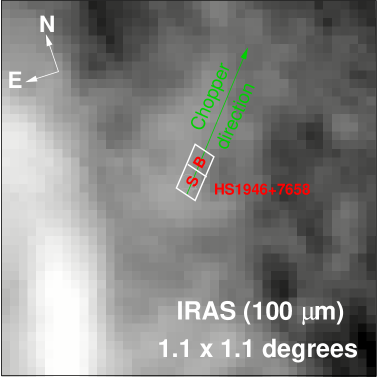
Figure 4: IRAS observation at 100 $\mu$m of a sky region of 1.1$\times$1.1 degrees around the source HS 1946+7658, whose position is indicated by S. The sky region where the background was measured is indicated by B. The white polygon represents approximatively the region observed by the C200 camera. The solid line indicates the chopper direction $\sim$41^∘ to the West of North.

The 150$\mu$m flux values for the high redshift source HS 1946+7658 differ by at least a factor of 6 between two epochs separated by less than a year (see Tables 5 and 6). Such extreme FIR variability is unlikely in a RQQ. The larger flux resulted from a chopped measurement, which is more susceptible at longer wavelengths to both background fluctuations and instrumental effects (e.g., a number of inadequately corrected cosmic ray strikes, unusually high detector drift, etc…) than the raster maps. Fig. 4 shows a 1.1$\times$1.1 degree region around HS 1946+7658 at 100$\mu$m from IRAS, with the position of the source and the ISOPHOT chopper direction indicated. Bright cirrus structures are nearby, and the background ranges from 0.21 – 0.38 MJy/sr within 90″of the source (equivalent to 0.16 – 0.28 Jy on the C200 covered area) (IRSKY version 2.5). A strong gradient in the direction SE–NW in the background emission is clearly shown, which coincides with the ISOPHOT chopper direction. These variations may be greater at longer wavelengths and with the better spatial resolution of ISOPHOT. As a consequence of the uncertainties for this source, chopped data at $\lambda$ $>$ 100$\mu$m for HS 1946+7658 will not be included in subsequent analysis.

The result of this method suggests that for all the selected objects, with the exception of PKS 0637$-$752, the IR emission is thermal in origin. The result is not very strong since a non-thermal process may also produce a constant flux. However, it is unlikely to measure the same flux from a non-thermal source during three different observations performed in a range of 14 years (from 1983 to 1997) as observed in six objects (see Fig. 3).

The third test is the simplest, and it can be applied to the whole sample since a broad spectral coverage from radio to the IR is available for all the sources. Before applying this test we need to estimate the contribution from the non-thermal component in the IR and subtract it from the observed IR spectrum. The non-thermal contribution can be estimated by fitting the radio data with a reasonable model and then extrapolating it to higher frequencies (see next section).

4.2 Contribution of the radio non-thermal component in the infrared

In order to estimate the contribution of the radio non-thermal component in the IR domain, the radio continuum was fitted with some plausible models, and extrapolated to higher frequencies. In the following we will distinguish two components in the radio spectra of RLQ, the extended component (radio lobes), and the core component (unresolved core, jet, etc…).

The radiation emitted by compact sources, like the cores and the hot-spots of radio loud objects, can be modeled by a self-absorbed synchrotron emission spectrum. In the case of a homogeneous plasma with isotropic pitch angle distribution and power law energy distribution of the form $N(E)\!\propto\!E^{-s}$, this can be expressed as:

$$L_{\nu}\propto\left(\frac{\nu}{\nu_{\mathrm{t}}}\right)^{\alpha_{\mathrm{1}}}\cdot\left[1-\exp\left(-\left(\frac{\nu_{\mathrm{t}}}{{\nu}}\right)^{\alpha_{\mathrm{1}}-\alpha_{\mathrm{2}}}\right)\right]\cdot e^{-\frac{\nu}{\nu_{\mathrm{cut\,off}}}},$$ (2)

where $\nu_{\mathrm{t}}$ is the frequency at which the optical depth of the plasma is equal to unity, and $\nu_{\mathrm{cut\,off}}$ is the frequency corresponding to the cut off energy of the plasma energy distribution, at which the energy gains and losses of the electrons are equal. The optically thick and optically thin spectral indices are denoted by $\alpha_{\mathrm{1}}$, and $\alpha_{\mathrm{2}}$. In the case of a homogeneous source, $\alpha_{\mathrm{1}}$ is expected to be 2.5, and $\alpha_{\mathrm{2}}$ is related to the exponent $s$ of the plasma energy distribution by the relationship: $\alpha_{\mathrm{2}}=-(s-1)/2$. The superposition of several self-absorbed components can produce a flatter power law. In this case the spectral model of equation (2) will remain valid, but $\alpha_{\mathrm{2}}$ will not have the same meaning. If the source is optically thin, as in extended sources (radio lobes), the emitted spectrum can be expressed more simply as:

$$L_{\nu}\propto\left(\frac{\nu}{\nu_{\mathrm{cut\,off}}}\right)^{\alpha_{\mathrm{2}}}\cdot\mathrm{e}^{-\frac{\nu}{\nu_{\mathrm{cut\,off}}}}.$$ (3)

In many cases the contribution of the synchrotron component at high frequencies is negligible compared to the observed emission, therefore a high energy cut off was not included in the model. The model is then represented by a broken power law of slopes $\alpha_{\mathrm{1}}$ and $\alpha_{\mathrm{2}}$, or by a simple power law of slope $\alpha_{\mathrm{2}}$, according to the presence/absence of self absorption.

The synchrotron model describes well the observed radio spectra of most of the sources in the sample. However, while in the case of SSRQ it is quite easy to separate the different components and hence apply a model for each of them, the spectral modeling is more difficult for FSRQ. For these sources we parameterize the emitted spectrum with an empirical equation that is valid if the resulting spectrum is produced by self-absorbed synchrotron emission or by optically thin synchrotron emission due to a hard electron spectrum produced through the acceleration processes in turbulent plasma (Wang et al. (1997)). The observed flat radio spectra are described by the following equation:

$$L_{\nu}\propto\left(\frac{\nu}{\nu_{\mathrm{b}}}\right)^{\alpha_{\mathrm{1}}}\cdot\frac{\left[1-\exp\left(-\left(\frac{\nu_{\mathrm{t}}}{{\nu}}\right)^{\alpha_{\mathrm{1}}-\alpha_{\mathrm{2}}}\right)\right]}{\left[1-\exp\left(-\left(\frac{\nu_{\mathrm{b}}}{{\nu}}\right)^{\alpha_{\mathrm{0}}-\alpha_{\mathrm{1}}}\right)\right]}\cdot\mathrm{e}^{-\frac{\nu}{\nu_{\mathrm{cut\,off}}}},$$ (4)

where $\nu_{\mathrm{b}}$ is the frequency at which the spectrum flattens, $\alpha_{\mathrm{0}}$ is the spectral index observed at low frequencies ($\nu<\nu_{\mathrm{b}}$), and the other model parameters have the same meaning as in equation (2).

The observed SEDs from the radio to the mm energy domains were fitted with one or a combination of these models (see best fit parameters in Table 7).

Table 7: Best fit parameters of non-thermal models

Source Name	Model†	$\alpha_{\mathrm{0}}$	$\alpha_{\mathrm{1}}$	$\alpha_{\mathrm{2}}$	$\nu_{\mathrm{t}}$	$\nu_{\mathrm{cut\,off}}$
Source					(109 Hz)	(1014 Hz)
3C 47 (Core)	$b$		1.64	$-$0.45	2.98
3C 47 (Lobe)	$c$			$-$0.99
PKS 0135$-$247	$d$	$-$0.78	0.30	$-$0.80	69.52	2.00
PKS 0408$-$65	$c$			$-$1.19
PKS 0637$-$752	$d$	$-$0.60	0.55	$-$0.78	37.20	4.49
PKS 0637$-$752 (Low)	$e$	$-$0.55	0.55	$-$1.50	75.12
PKS 0637$-$752 (High)	$d$	$-$0.60	0.49	$-$0.78	41.28	4.22
PG 1004+130 (Core)	$b$		0.53	$-$0.19	2.00
PG 1004+130 (Lobe)	$c$			$-$0.80
4C 61.20 (Core)	$b$		0.20	$-$0.15	20.00 (F)
4C 61.20 (Lobe 1)	$c$			$-$1.04
4C 61.20 (Lobe 2)	$c$			$-$0.93
PG 1048$-$090 (Core)	$b$		0.50	$-$0.65	20.00 (F)
PG 1048$-$090 (Lobe)	$c$			$-$0.84
PG 1100+772 (Core)	$b$		0.15	$-$0.80	11.00
PG 1100+772 (Lobe)	$c$			$-$0.83
PG 1103$-$006 (Core)	$b$		0.30	$-$0.50	20.00 (F)
PG 1103$-$006 (Lobe)	$c$			$-$0.70
PG 1216+069	$a$		0.76	$-$0.09	0.96	20.39
PG 1543+489	$c$			$-$0.90
PG 1718+481	$b$		0.58	$-$0.34	11.45
B2 1721+34	$c$			$-$0.69
3C 405 (Core)	$a$		0.50 (F)	$-$0.74	126.00 (F)	3.58
3C 405 (Lobe 1)	$c$			$-$1.26
3C 405 (Lobe 2)	$c$			$-$1.30
B2 2201+31A (Low)	$d$	$-$0.52	0.60	$-$0.30	28.60	0.034
B2 2201+31A	$d$	$-$0.44	0.50	$-$0.50	34.89	0.24
PG 2214+139	$c$			$-$0.92
PG 2308+098	$c$			$-$0.85

^† Model $a$ corresponds to equation (2), and model $b$ to the same equation without cut off;
   model $c$ corresponds to a simple power law; model $d$ to equation (4), and model $e$ to the
same equation without cut off.
(F) indicates a fixed value.

In some cases near-IR data have also been used in the fits, in particular when no data in between mm and near-IR frequencies constrained the spectrum to lie below the near-IR flux (PKS 0135$-$247, PKS 0637$-$752, 4C 61.20, PG 1004+130, PG 1216+069, PG 1718+481, 3C 405, and B2 2201+31A). In a few cases we fixed some model parameters, as indicated in a footnote of table 7, since the available data could not constrain them. The fixed values were chosen in the range of values that provided reasonable spectra with properties similar to those observed in other sources. Model $a$ in Table 7 corresponds to equation (2). It was applied for modeling core spectra of PG 1216+069, and 3C 405. The same model without the cut off ($b$) was applied for modeling weak core spectra for which the high energy cut off was not constrained (3C 47, PG 1004+130, 4C 61.20, PG 1048$-$090, PG 1100+772, PG 1103$-$006, and PG 1718+481). A simple power law model ($c$) was used to fit the radio emission from the lobes of SSRQ and RG (3C 47, PKS 0408$-$65, PG 1004+130, 4C 61.20, PG 1048$-$090, PG 1100+772, PG 1103$-$006, B2 1721+34, 3C 405 and PG 2308+098) and the radio emission of RQQ (PG 1543+489, and PG 2214+139). Simultaneous observations available in the literature generally do not provide wide or well-sampled wavelength coverage, so all available data were used in the fits to the SEDs. The data and analysis are adequate for the central purpose of estimating the contribution of the non-thermal component to the IR emission. The model $d$, corresponding to equation (4), was applied to fit the radio emission of FSRQ (PKS 0135$-$247, PKS 0637$-$752, and B2 2201+31A). The value of the break frequency $\nu_{\mathrm{b}}$ was arbitrarily fixed to 2.75 GHz, since it provides a good fit to the emitted spectrum of the three objects. In the case of PKS 0637$-$752 (Low) (see section 4.2.1) the cut off was not included in the model ($e$) since the high frequency part of the spectrum is very steep.

4.2.1 Uncertainties in the radio contribution estimate

The location of the high energy cut off is difficult to establish. Every power law relative to the optically thin emission was extended at higher frequencies until the spectrum turned down, and hence a cut off was required by the data. A spectral cut off was thus required only in five objects (PKS 0135$-$247, PKS 0637$-$75, PG 1216+069, 3C 405, and B2 2201+31A), but it could have been located at lower frequencies and present in other objects, too. In most of the cases this parameter does not affect the presence and the strength of the remaining IR flux, but its energy value may be important in FSRQ (PKS 0135$-$247, PKS 0637$-$75, and B2 2201+31A), since these objects have flat radio spectra for which extrapolation up to IR frequencies is comparable to the IR fluxes. For these sources a more accurate analysis of their radio spectra is needed. Since PKS 0135$-$247 was not detected in the IR, no further analysis can be performed. We concentrate only on PKS 0637$-$75 and B2 2201+31A. In order to better constrain the non-thermal radio spectrum, i.e. to find some evidence of a spectral cut off at sub-mm/far-IR frequencies, we searched in the literature for simultaneous observations at these wavelengths, and we selected those that showed the flattest and the steepest spectrum. For PKS 0637$-$75 the flattest mm power law, chosen among several simultaneous observations (Tornikoski et al. (1996)), was measured on February 15th, 1990 ($\alpha$(3.0-1.3 mm) = $-$0.77), and the steepest one was measured on April 4th, 1991 ($\alpha$(3.0-1.3 mm) = $-$1.47). The two power laws are reported in Fig. 2b with a dashed, and a dashed-dotted line, respectively, plus displayed separately with flattest (Fig. 2c) and steepest (Fig 2d) spectral fits. The flattest spectrum overlaps the observed IR spectrum, leaving no additional IR component. On the contrary, the extrapolation of the steepest spectrum to IR frequencies is clearly below the observed IR spectrum, but the IR observations were not simultaneous to the mm observations. The source was observed by IRAS in 1983, and by ISO at different wavelengths in 1997. During the elapsed time the source became fainter in the far-IR, while shorter wavelength data from the two diferent epochs are consistent. In the following we will suppose that a thermal IR component is present, but dominating only at $\lambda<$60 $\mu$m, and we will analyze its properties and compare them with those observed in other sources.

For B2 2201+31A the flattest mm power law ($\alpha$(1.0-0.87 mm) = $-$0.09) was measured on February 1989 (Chini et al. 1989a ), and the steepest one was measured on September 14th, 1993 ($\alpha$(2.0-1.3-1.1 mm) = $-$0.72). The two power laws are reported in Fig. 2e with a dashed, and a dashed-dotted line, respectively. The spectrum is in both cases quite flat, however the extrapolation of the 1993 spectrum lies below the IR spectrum. More than the sub-mm data, the analysis of the emission at shorter wavelengths gives important indications on the origin of the IR emission. B2 2201+31A was observed on September 15th, 1993 also in the near-IR (simultaneous sub-mm and near-IR data are indicated by large open circles in Fig. 2e). The near-IR data are above the extrapolation of the sub-mm data, suggesting the presence of two different spectral components in these two wavelength ranges (see the analogous case of 3C 273 in Robson et al. (1986)). This hypothesis is also suggested by the constant emission observed up to 60 $\mu$m. A non-thermal source is expected to vary more at higher frequencies, due to greater energy losses. All these considerations suggest the short wavelength continuum is dominated by a thermal component. As in the case of PKS 0637$-$75 we will suppose that an additional IR thermal component is present at $\lambda\,\leq$ 60 $\mu$m.

These two sources (PKS 0637$-$752, and B2 2201+31A) are good examples of how variability can create an artificial IR spectral turnover, or hide a real one. An IR spectral turnover may be due to different luminosity states of the source at different epochs, instead of to the presence of a separate IR component. The weakness of the radio emission in RQQ precludes that its extrapolation could account for the IR emission for all reasonable assumptions on the radio variability. In SSRQ the extrapolation of the radio component in the IR is usually too faint to explain the IR emission, even if we take into account variability. The variability factors observed in two SSRQ in our sample, 3C 47 and PG 1004+130, are too small to explain the much higher IR fluxes, and this is probably true for the SSRQ in general. In the mm domain we measured a flux variation from the core of the SSRQ 3C 47 of a factor of $\sim$ 2 in almost three years (the emitted flux density at $\sim$ 100 GHz was equal to 16.3$\pm$0.9 mJy on September 1995 (van Bemmel et al. (1998)), and equal to 30.8$\pm$0.6 mJy on July 1998 (this work)). The SSRQ PG 1004+130 was observed twice at 6 cm, in 1982 and in 1984, with a flux variation of a factor $\sim$2.5, from 12 mJy to 30 mJy (Lister et al. (1994)).

In conclusion, the radio models shown in Fig. 2 indicate the presence of an additional IR component in almost the whole sample. According to the third test, this result indicates that the observed IR emission is of thermal origin. The properties of the IR emission in quasars will be derived and analyzed in section 4.3, after subtraction of the non-thermal contribution extrapolated from the radio domain.

4.3 Modeling of the IR component

The IR emission can be accounted for by reradiation of the central luminosity by gas and dust in warped discs in the host galaxies of the quasars (Sanders et al. (1989)), in the outer edge of the accretion disc and in a torus of molecular gas within a few parsecs of the central energy source (Niemeyer & Biermann (1993); Granato & Danese (1994); Granato et al. (1997); Pier & Krolik (1992), 1993), and/or by starburst emission (Rowan-Robinson (1995)). The host galaxy starlight contribution is probably negligible in the far/mid-IR since the host galaxy spectrum largely differs in shape and luminosity from the SED of the selected objects (see Fig. 2). We describe here the main observational properties of the different objects of each class and compare them using a very simple model of thermal emission: the grey body model. This model does not take into account the source geometry (toroidal, warped disc, etc). An isothermal grey body at the temperature T emits at frequency $\nu$ a luminosity density given by the following equation (Gear (1988), Weedman (1986)):

$$L_{\nu\,\mathrm{em}}=4\pi^{2}r^{2}\cdot\mathrm{B}(\nu_{\mathrm{em}},\mathrm{T})\cdot(1-e^{-\tau_{\mathrm{d}}}),$$ (5)

where $r$ is the radius of the projected source, B($\nu$,T) is the Planck function for a blackbody of temperature T, and $\tau_{\mathrm{d}}$ is the optical depth of the dust. The optical depth can be approximated by a power law of type $\tau_{\mathrm{d}}$ = $(\nu/\nu_{\mathrm{0}})^{\beta}$, where $\nu_{\mathrm{0}}$ is the frequency at which the dust becomes optically thin, and $\beta$ is the dust emissivity index. A non-linear least squares fit was used in the fitting procedure, leaving the radius $r$, the temperature T, and the frequency $\nu_{\mathrm{0}}$ free to vary , while the emissivity exponent $\beta$ was fixed equal to 1.87 (Polletta & Courvoisier (1999)).

Figure 5: SEDs as $\nu L_{\nu}$ versus $\nu$ in the rest frame of the objects (2 FSRQ, 2 RIQ, 1 RG, 1 RQQ). Symbols as in Fig. 2. Dotted lines represent the best fit non-thermal models of the radio component and the best fit grey body models of the IR component. The temperature of each grey body component is reported. The sum of all single fitted models is shown by a solid line.

Figure 5: Continued (6 SSRQ).

Figure 5: Continued (6 RQQ).

The observed IR SEDs are smooth and indicate a wide and probably continuous range of dust temperatures, describable by several grey body components. The best fit grey body models of the observed IR SEDs are shown in Fig. 5. The thick solid line represents the sum of non-thermal and grey body components. Each individual component is represented by a dotted line. The temperature (T) and the size (r) of each grey body component are listed in columns 5–10 of Table 8. It is worth noting that we could fit the observed IR spectra using a different optical depth function (different $\beta$, and $\nu_{\mathrm{0}}$ values). The optical depth value is important in a discussion of the source geometry in terms of an extended or compact heating source. In our models the optical depth values derived by the fits are low ($<\,$1) in the far/mid-IR, and $\simeq$1 in the near-IR ($\sim$ 3$\mu$m). If the dust becomes optically thin at longer wavelengths, the real source sizes will be smaller than our estimates, and vice versa. Using our optical depth values, the estimated sizes of the observed dust components range between 0.06 pc and 9.0 kpc, and the temperatures between 43 K and 1900 K. The minimum temperature may be due to an absence of dust at large distances (few kpcs) or at low temperature, and/or to starlight heating to the orders of the inferred minima. The maximal temperature is generally explained as a drop in opacity caused by the sublimation of the most refractory grains at temperatures T $\sim$ 2000 K (Sanders et al. (1989)). The total luminosities observed in the IR, obtained by integrating the grey body components (see column 1 in Table 8), vary over a wide range, from 2.0$\cdot$10¹¹ $L_{\mathrm{\odot}}$ to 7.6$\cdot$10¹³ $L_{\mathrm{\odot}}$. No significant difference in the distribution of sizes, temperatures, and luminosities are observed among different types of quasars.

Table 8: Best fit parameters of grey body models

Source Name	Total L(IR)	$\frac{L(60-200\mu m)}{L(3-60\mu m)}$	Log(Md)	I Component		II Component		III Component
	(1011 L⊙)		(M⊙)	T (K)	r (pc)	T (K)	r (pc)	T (K)	r (pc)
3C 47	36.1	0.205	7.55	42.7	7621	208	109
PKS 0637$-$752 (Low)	58.6	0.056	6.68	61.0	1923	219	276
PG 1004+130	11.6	0.040	5.35	92.6	663	421	12
4C 61.20	29.8	0.086	6.14	86.8	1401
PG 1100+772	14.1	0.024	5.38	74.9	597	174	49	696	2.16
PG 1103$-$006	25.3	0.024	5.18	120.0	496			1322	0.33
PG 1216+069	28.8	0.007	4.76	115.8	310	511	8
PG 1352+183	3.8	0.091	5.26	80.9	556			1584	0.11
PG 1354+213	9.3	0.001				211	23	898	0.98
PG 1435$-$067	2.8						4	465
PG 1519+226	3.8	0.097	5.97	50.7	1264	168	41	591	1.34
PG 1543+489	49.9	0.202	7.54	46.0	8997	165	183	561	5.17
PG 1718+481	105.3	0.007	5.06	141.5	573			878	3.60
B2 1721+34	8.6	0.047	5.36	80.0	611	230	32	1800	0.11
HS 1946+7658	761.5	0.006	6.00	130.8	1294	528	37
3C 405	4.6	0.137	5.79	67.7	1265	184	13
B2 2201+31A (Low)	19.5	0.002				222	18	611	3.99
PG 2214+139	2.0	0.091	5.22	63.7	540	399	3	1900	0.06
PG 2308+098	11.1						6	569

We also derive the mass of each dust component at the measured temperature, using the following equation (Hughes et al. (1997)):

$$\mathrm{M}_{\mathrm{d}}=\frac{L_{\nu\,\mathrm{em}}}{K_{\mathrm{d}}(\nu_{\mathrm{emis}})}\frac{1}{\mathrm{B}(\nu_{\mathrm{emis}},\mathrm{T})},$$ (6)

where $K_{\mathrm{d}}(\nu_{\mathrm{emis}})\propto\nu^{\beta}$, $\beta$ = 1.87, is the rest-frequency dust absorption coefficient. The normalization is $K_{\rm d}(\nu_{\rm emis})=10\;{\rm cm}^{2}{\rm g}^{-1}$ at 250 $\mu$m (Hildebrand (1983)), giving $K_{\mathrm{d}}(\nu)$ = 1.14 cm² g^-1 at 800 $\mu$m. The range of assumed values of $K_{\mathrm{d}}(\nu)$ at 800 $\mu$m in the literature is 0.4–3.0 cm² g^-1 (Draine & Lee (1984); Mathis & Whiffen (1989)). Our dust mass estimates can thus differ by, at most, a factor 2.7. The derived values of dust masses are reported in column 4 of Table 8, and, separately for each class, in Fig. 6. Since the largest dust masses are located in the outer, less illuminated, lower temperature regions of the dust distribution, M_d is mainly constrained by far-IR data. Therefore, when sub-mm and far-IR data are not available, the real dust mass cannot be well measured. For this reason we did not report the dust and gas masses when the low temperature component was not constrained. The absence of data in the near-IR has a negligible effect on the dust mass estimate. As for the other parameters (T, L(IR), r), the dust mass distribution does not differ significantly among different types of quasars (see Fig. 6).

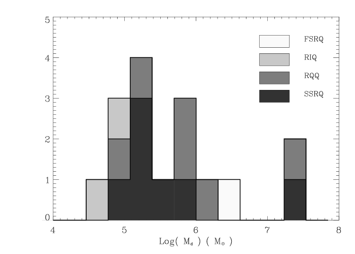
Figure 6: Histogram of the dust masses for the different classes: RQQ, SSRQ, FSRQ, and RIQ.

5 Similarities and differences in the SED of RLQ and RQQ

The present sample contains a range of radio source classifications, with which we can elucidate the dependence of broad-band spectral features on radio properties, thereby testing some unification scenario predictions. The limitations of these tests lie in the sample’s relatively small size and heterogeneous nature.

5.1 Average SED

A quick look at the main spectral differences between the different kinds of quasars is provided by the comparison of the average SED of RQQ, RIQ, FSRQ, and SSRQ (including the RG 3C 405). The SEDs are shown in $L_{\nu}$–$\nu$ and $\nu$L_ν–$\nu$ spaces separately for each class over the radio/soft X-ray frequency range in Fig. 7.

Figure 7: The average quasar energy distribution for RQQ (solid line), RIQ (dotted line), FSRQ (dashed line), and SSRQ (dash-dot line). The number of objects that were used in each class is reported on the figure with the class name. A symbol is reported for each frequency bin, if at least one data point is available. The two high redshift objects of the sample: HS 1946+7658, and PG 1718+481, were excluded since they are characterized by very high luminosities that modify the average SEDs at a few frequencies producing an irregular spectral shape. Two host galaxy templates are also reported: a typical spiral galaxy (dash-dot-dot-dot line), and a giant elliptical galaxy (long dashed line). No normalization was applied to the reported curves.

The broad spectra of two typical host galaxies (a giant elliptical and a spiral galaxy), in their rest frames and without any normalization, are also plotted in Fig. 7, as in Fig. 2. The average SEDs have been computed using the conventional mean, excluding upper limits. The width of each frequency bin is equal to 0.5 in Log($\nu$). The reported uncertainties correspond to the standard deviation of the mean of the data per frequency bin. All the data have been connected by straight lines. At soft X-ray energies we indicate the average power law $\pm$ 1$\sigma$ computed from the distribution of best fit soft X-ray power law models of all objects of the same class (photon index $\Gamma$ = 2.73$\pm$0.61 (RQQ), 2.39$\pm$0.19 (RIQ), 2.39$\pm$0.23 (SSRQ), and 2.25$\pm$0.12 (FSRQ)).

As expected, the largest difference in luminosity among the different classes appears at radio wavelengths. A smaller difference is observed at soft X-ray energies, and in the near-IR ($\nu>$ 10¹⁴ Hz corresponding to $\lambda<$ 3 $\mu$m), while the luminosity and the spectral shape in the mid- and far-IR are remarkably similar (see Fig.7). The large difference in the IR spectral shape between quasars and the host galaxy templates indicates that the contribution from the host galaxy is negligible also at radio and soft X-ray energies, and not only in the far/mid-IR. This result is in agreement with previous studies on the broad SED of quasars (Sanders et al. (1989); Elvis et al. (1994)). A quantitative comparison of the luminosity emitted at different frequencies by each quasar class is presented in the next section.

5.2 Multi band luminosities

The IR component was also modeled by fitting a parabola in Log L_ν–Log $\nu$ space (see Fig. 2). The parabola model gives a rough estimate of the strength and shape of the IR component, even if the spectral coverage is not complete. For several objects upper limits were also used in the fit. This model has by itself no physical meaning, however, it describes the IR component relatively well, it can easily be traced even with poor spectral coverage, and can take into account the whole IR emission of most of the objects in a larger wavelength range than the detailed grey body models. The parabola is too narrow to satisfy the observed IR SED in a few cases, e.g., in 3C 405 and PG 1543+489. In these cases we fitted only the far/mid-IR data where the IR emission usually peaks. The parabola parameters are its width, the frequency of maximum luminosity density ($\nu_{\mathrm{peak}}$) and the maximum luminosity density ($L_{\nu_{\mathrm{peak}}}$). The parabola fit to the IR component was applied to all objects of the sample, except PKS 0135$-$247, for which no IR data are available (see Fig. 2a). The distribution of the peak frequencies values ($\nu_{\mathrm{peak}}$) observed in the four different classes of objects is reported in Fig. 8. The distribution is quite similar for SSRQ and RQQ, ranging from 2.6$\cdot$10¹² Hz (114 $\mu$m) to 3.6$\cdot$10¹³ Hz (8 $\mu$m), while it is shifted to higher frequencies for FSRQ and RIQ, ranging from 9.0$\cdot$10¹² Hz (33 $\mu$m) to 2.8$\cdot$10¹³ Hz (11 $\mu$m). This difference may be due to the flat radio non-thermal component extending to high frequencies in FSRQ and RIQ, and dominating the dust emission.

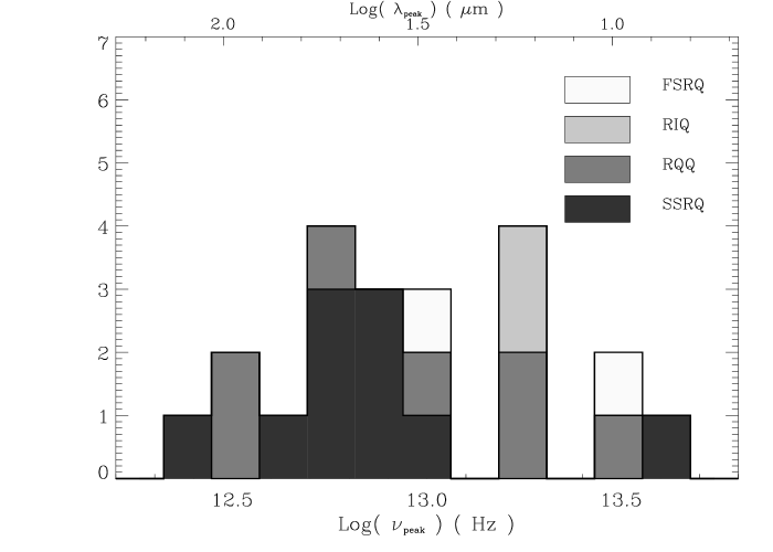
Figure 8: Histogram of the IR peak frequency of the parabola model for the different classes: RQQ, SSRQ (including the RG 3C 405), FSRQ, and RIQ.

We define the IR luminosity $L\mathrm{(IR)}$ as the product of the luminosity value at which each parabola peaks and the corresponding frequency ($L$(IR) = $\nu_{\mathrm{peak}}\cdot L_{\nu_{\mathrm{peak}}}$). Note that this parameter does not depend on the width of the parabola. Only upper limits for $L\mathrm{(IR)}$ could be derived for PKS 0408$-$65 and PG 1040$-$090. The distribution of $L\mathrm{(IR)}$ is reported in Fig. 9. In this, and in the following histograms upper limits are shown with arrows, one per object. The similarity in the IR luminosities and spectra (see also Fig. 7) in all quasars suggest a similar origin.

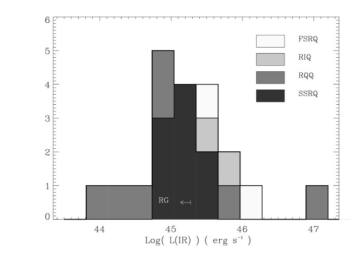
Figure 9: Histogram of the peak luminosity of the IR parabola model for the different classes: RQQ , SSRQ (including the RG 3C 405 whose position is indicated), FSRQ, and RIQ.

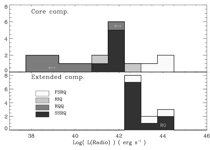
Figure 10: Histogram of the core and extended components radio luminosity for the different classes: RQQ, SSRQ (including the RG 3C 405 whose position is indicated), FSRQ, and RIQ.

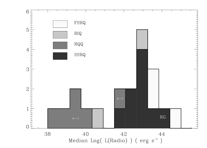
Figure 11: Histogram of the median radio luminosity for the different classes: RQQ, SSRQ (including the RG 3C 405 whose position is indicated), FSRQ, and RIQ.

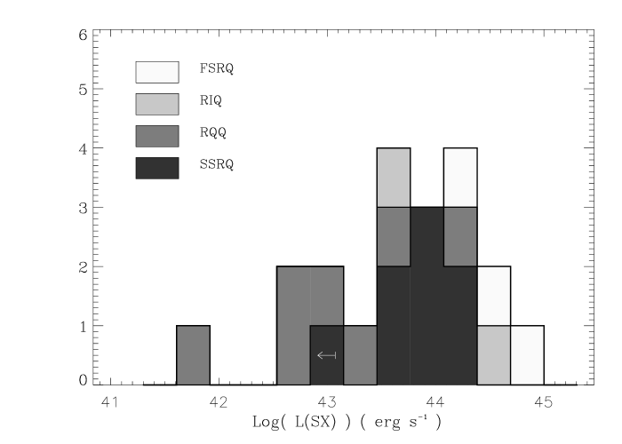
Figure 12: Histogram of the soft X-ray luminosity at 1 keV for the different classes: RQQ, SSRQ, FSRQ, and RIQ.

The radio emission in the RLQ arises from two very different spatial scales, the core and extended components. We calculated the average of $\nu$L_ν over the rest-frame interval 5–9 GHz for each spatial component in all of the RLQ, except PG 1354+213 and HS 1946+7658, which were undetected at these frequencies. Fig. 10 displays histograms for the two components separately, and Fig. 11 shows the distribution of the median of all measured $\nu$L_ν over the same frequency range, without component distinction. The distribution of the median radio luminosity is bi-modal (Fig. 11). However, if we consider only core radio luminosities (top panel of Fig. 10), the SSRQ radio luminosity distribution shifts towards lower values, making a continuous distribution, rather than a bi-modal one, but without overlapping. The contribution from the extended components are very similar in FSRQ and SSRQ (bottom panel of Fig. 10). In the following analysis we will consider only the core luminosity $L\mathrm{(Radio)}$. When the core luminosity is not available (PKS 0408$-$65, B2 1721+34, 3C 405, and PG 2308+098), we report an upper limit corresponding to the average radio luminosity relative to the extended component.

In the soft X-ray, we define $L$(SX) as $\nu$L_ν with $\nu$ corresponding to 1 keV in the observer’s rest-frame. The distribution of $L$(SX) for each class is reported in Fig. 12. In the soft X-ray, no data are available for 3C 405, and PKS 0408$-$65, and only an upper limit is available for PG 1004+130.

5.3 Origin of the observed luminosities

The main factors determining the observed luminosities are: the energy emitted by the central engine (AGN); the amplification due to Doppler boosting in a relativistic jet; and the contribution from a starburst. We will estimate the role of each of these parameters in producing the SEDs through the comparison of the observed radio, IR, and soft X-ray luminosities, represented by $L$(Radio), $L$(IR) and $L$(SX), respectively (see section 5.2 for their definition).

5.3.1 Orientation effects in RLQ

The orientation of the beamed emission can be estimated from the radio core fraction R. This quantity, defined as the ratio between the core radio luminosity and the luminosity of the extended radio emission at 5–9 GHz in the rest frame, serves as an orientation indicator of the radio source with respect to the observer, measuring the relative strength of the core component (Hes et al. (1995)). The core flux was not available for three SSRQ and one RG, thus the parameter R was not computed. In the case of FSRQ we computed the luminosity of the extended component in the frequency range 5–9 GHz by extrapolating the power law observed at low frequencies (power law index $\alpha_{\mathrm{0}}$ in Table 7).

Figure 13: Luminosity emitted in the soft X-ray, radio and IR domains compared to the parameter R given by the ratio between the radio luminosity of the core and of the extended components. The different symbols correspond to different classes of objects: squares for SSRQ, and circles for FSRQ. The dashed lines are the best fit lines.

The FSRQ are well separated from SSRQ in the distribution of the ratio R (see Fig. 13). This difference permits us to estimate the enhancement factor of the beamed emission after a few considerations. First, the observed radio emission in RLQ is mainly produced by the jet and its core rather than a starburst, since star-emitting ULIRG have much lower radio luminosity than RLQ (Colina & Pérez-Olea (1995)). Second, we assume that the radio source is intrinsically identical in FSRQ and SSRQ, and that the difference in their radio emission is due only to the orientation of the beamed emission. After these approximations we can write

$$L\mathrm{(Radio\;Core)}_{\mathrm{FSRQ}}=A\cdot L\mathrm{(Radio\;Core)}_{\mathrm{SSRQ}}$$ (7)

where $A$ is the amplification factor of the beamed emission. Since the luminosity of the extended components are the same for the flat and steep radio quasars (see above), using equation (7) we can derive a relation between the parameters $R_{\mathrm{FSRQ}}$ and $R_{\mathrm{SSRQ}}$: $R_{\mathrm{FSRQ}}$ = $A\cdot R_{\mathrm{SSRQ}}$. Replacing the observed values of $R_{\mathrm{SSRQ}}$ ($\simeq$ 0.05–0.15), and $R_{\mathrm{FSRQ}}$ ($\simeq$ 3–4) (see Fig. 13) in the above relation yields $A$ $\simeq\,$20–80.

Fig. 13 displays $L$(Radio), $L$(SX), and $L$(IR) versus the core fraction R. Linear correlation results for these relations are reported in Table 9, where the parameter pairs are reported in the first two columns, the number of data pairs in the third, in column 4 the linear correlation rank (r_l), and in column 5 the associated probability to have such a correlation rank from uncorrelated values (P_l).

Table 9: Correlation test results for FSRQ and SSRQ

X	Y	N	$r_{\mathrm{l}}$	Pl (%)
Log($L$(IR))	Log(R)	7	0.53	25.
Log($L$(Radio))	Log(R)	9	0.94	0.03
Log($L$(SX))	Log(R)	8	0.73	6.0

Higher radio and soft X-ray luminosities are observed in objects with higher values of the radio core fraction R (when the jet points towards us). The orientation effect is more important in the radio domain, as shown by the stronger correlation, than in the soft X-ray, and negligible in the IR. This implies that the radio core and a fraction of the total emitted soft X-ray luminosities are emitted anisotropically. We furthermore verified that R is not correlated with the redshift and thus that the above result is not an artifact of distance related biases in the measurement of R.

Assuming that the soft X-ray source is intrinsically identical in FSRQ and SSRQ, the observed difference in L(SX) arises from the orientation of the fraction, $f$, that is beamed. If the fraction of emitted radiation that is beamed is enhanced by a factor A, identical to that of the radio emission, the following relation between the soft X-ray luminosity in FSRQ and that in SSRQ will be valid:

$$L\mathrm{(SX)}_{\mathrm{FSRQ}}=A\cdot f\cdot L\mathrm{(SX)}_{\mathrm{SSRQ}}+(1-f)\cdot L\mathrm{(SX)}_{\mathrm{SSRQ}}.$$ (8)

Using the average value of the ratio $L\mathrm{(SX)}_{\mathrm{FSRQ}}/L\mathrm{(SX)}_{\mathrm{SSRQ}}$ that is $\approx 3.2\pm 2.2$, and the range of values obtained for the factor $A$, we derive a fraction $f\approx$ 3–12% for the beamed fraction of the soft X-ray component.

5.3.2 SSRQ $versus$ RQQ

The radio and the soft X-ray luminosities are mainly produced by the AGN component (see sections 5.1 and 5.3.1). The comparison between the luminosities emitted in the radio and soft X-ray domains is then equivalent to a comparison of the AGN power in the two types of quasars. The radio core emission of SSRQ is on average 200 times higher than that of RQQ (see Fig. 10) and the soft X-ray luminosity is on average 8 times higher in SSRQ than in RQQ (see Fig. 12). Since the SSRQ show luminosities higher than RQQ not only at radio and soft X-ray energies, but also in the hard X-ray domain (Lawson & Turner (1997)), we argue that the bolometric AGN luminosity is much higher in SSRQ than in RQQ. The difference in the AGN power should be observable at all frequencies where the AGN emission dominates. We have already pointed out the similarity in IR luminosities and spectra of SSRQ and RQQ (see Figs. 7 and 9). This similarity suggests that the origin of the dominant IR component is not AGN-related. The candidate is then a starburst.

Some indication of the dominant IR emission mechanism can be gleaned from the shape of the SED. An AGN can emit a significant fraction, often a majority, of its infrared luminosity at shorter wavelengths, $\lambda$ $<$ 60$\mu$m, as long as the obscuring columns are not so large as to be optically thick at these wavelengths. Starburst dominated galaxies, on the other hand, produce the bulk of their infrared emission at $\lambda$ $>$ 60$\mu$m. The ratio of the luminosities in these two wavelength regimes, $L$(60-200$\mu$m)/$L$(3-60$\mu$m), thus provides a rough estimate of the primary driver of the infrared component. A histogram of this ratio is presented in Fig. 14, in which only the sources having at least two grey body components with T $<$ 1000 K are included. For comparison, the luminosity ratio from an average SED of low reddening starburst galaxies (Schmitt et al. (1997)) is also indicated. All of the AGN in the sample have infrared luminosity ratios less than the starburst fiducial value (=0.76) by a factor or four or more (the maximum ratio is 0.20 corresponding to 27% of starburst contribution), suggesting that the infrared in these sources is dominated by the central engine. The RQQ and SSRQ have similar average ratios, 8% of the total IR emission is produced by a starburst.

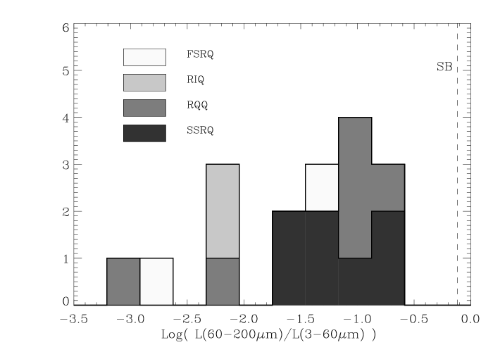
Figure 14: Histogram of the ratio $L$(60-200$\mu$m)/$L$(3-60$\mu$m) for the different classes: RQQ, SSRQ, FSRQ, and RIQ. The dashed line represents the value derived from the average SED of a sample of low reddening starburst galaxies.

Since the dominant IR source is the AGN, which differs in SSRQ and RQQ, other factors have to be taken into account to explain the similarity of their IR luminosities and average spectra. These factors can be the dust covering factor, its amount and geometric distribution. A higher dust covering factor in RQQ, due to larger total dust mass and/or a particular geometric distribution, may account for the similar IR radiation. Aspects of this hypothesis are attractive, since the presence of more circumnuclear material may be related to the physical conditions that hinder the jet formation and/or development in RQQ. However, if larger dust covering factors were present in RQQ, a higher probability to observe a RQQ through optically thick dust would be expected and a large fraction of RQQ with absorption features in the soft X-ray would be observed. Observations do not support these predictions (see section 2). Moreover, the similarity in the observed IR luminosities and spectra requires a fine tuning between the dust heating source, the dust amount and its geometric distribution, which makes this explanation improbable. We propose another scenario in which the dust properties (amount and distribution) and the heating source are similar in SSRQ and RQQ. The dust distribution contributing in the far-IR probably extends from the more external regions of the AGN, and is predominantly heated by the optical and UV radiation fields filling these external regions which are similar in both classes. At relatively large distances from the centre, the AGN components are similar in both types of quasars, towards the innermost regions, where the soft X-rays are emitted and a jet is formed, SSRQ and RQQ become different. The high energy photons escape from the centre without significant dust absorption and provide an important probe of the central radiation source. Observations indicate that the soft X-ray radiation is higher in SSRQ (see Fig. 7) in agreement with the proposed scenario.

From this analysis it is suggested that the main difference between RQQ, and SSRQ takes place in the innermost nuclear regions where the emitted power is higher in SSRQ than in RQQ, while the AGN external regions (dust distribution and optical/UV source) have similar properties in both types of quasars.

Since FSRQ and SSRQ show similar properties in the IR, once the non-thermal contribution is subtracted, this conclusion can be also extended to FSRQ.

6 Conclusions

Continuum observations from radio to soft X-ray energies have been presented for a sample of 22 quasars characterized by different degrees of radio emission. The IR data were obtained with ISOPHOT and IRAC1, and the mm data with IRAM, SEST and SCUBA. Further IR and mm data, and some radio and soft X-ray fluxes, were drawn from the literature. The availability of a broad band SED for several types of quasars allows us to separate the dominant spectral components in the radio and IR energy bands, and thus to compare their spectral properties in different types of quasars. The spectral analysis and the comparison of luminosities emitted in the radio, IR, and soft X-ray energy bands yields the following results:

1. What is the dominant mechanisms emitting at IR energies in RLQ and RQQ?

   In our quasar sample the dominant mechanism emitting in the far/mid-IR is thermal emission from dust heated by the optical and UV radiation produced in the outer regions of the AGN. A starburst contributes to the IR emission at different levels, but always less than the AGN ($\leq$27%). The presence of thermal IR emission in FSRQ remains rather uncertain. Among the three FSRQ of the sample we cannot derive any conclusion for two of them, and for a third one (B2 2201+31A) the observed data suggest a dominant thermal component at $\lambda\,\leq\,60\,\mu$m.

2. Do RLQ and RQQ have the same dust properties (temperature, source size, mass, and luminosity)?

   The equilibrium temperature of dust grains, the size and the mass of the dust distribution, and the emitted luminosity have been evaluated for all quasars. The estimated sizes of the observed dust components lie between 0.06 pc and 9.0 kpc, and the temperatures between 43 K and 1900 K. The total luminosity observed in the IR, obtained by integrating the grey body components, varies over a wide range: 2–760$\cdot$10¹¹ L_⊙. The amount of emitting dust in all types of quasars also varies in a broad range: 6$\cdot$10⁴–4$\cdot$10⁷ M_⊙. The distribution of any of these parameters does not differ significantly among the different types of quasars.

3. Does an interplay between the radio and the IR components exist?

   A bright and flat non-thermal component can be sufficiently strong in the IR to mask the dust emission in some sources, particularly FSRQ. However, this does not mean that the dust emission is absent. After subtracting an IR synchrotron component extrapolated from the radio, the residual IR emission had similar spectral shape and luminosity, regardless of the radio properties.

These results are based on the analysis of a small sample, and have to be confirmed by the study of larger samples. ISOPHOT has doubled the number of quasars with IR detections in the sample presented here. A great deal of additional progress on understanding the IR properties of quasars is expected when all of the quasar data available in the ISO archive will be fully analyzed and studied.