Can Rotational Properties of General Relativistic Compact Objects Be Predicted from Static Ones?

Abstract

Abstract. We propose an approximate description of basic parameters (radius, mass and oblateness) of general relativistic compact rotating objects in terms of the parameters of the static configuration and of the angular velocity only. The representation in terms of static properties is derived using the condition of stationary equilibrium together with some phenomenological assumptions. The predicted radius and mass of rotating neutron star (described by some realistic equations of state) and strange star (described by the bag model equation of state) are compared with data obtained by numerical integration of gravitational field equation.The obtained formulae also allow a simple derivation of the ”empirical” equation relating the maximum rotation frequency $\Omega_{max}$ of uniformly rotating star models to the mass and radius of the maximum allowable mass configuration of the non-rotating model.

Pacs Numbers:

I INTRODUCTION

Rotation is a basic physical property of astrophysical objects. Study of rotational properties of stars can lead to some restrictions imposed on the nuclear equation of state of dense matter at densities larger than nuclear density.Oscillations of rapidly rotating stars can become unstable hence producing detectable gravitational wave emissions.

In the past decades there were numerous attempts to construct analytic models for rotating perfect fluid bodies in general relativity. But obtaining an exact interior solution for a rotating body proved to be a formidable task.The first step in this direction was the fundamental result of Kerr [1] who obtained the solution for the vacuum domain, outside the rotating star. It took no less than three decades of investigations to obtain the first, highly idealized model of a general relativistic, thin rotating disk of dust, by Neugebauer and Meinel [2]. Various schemes have been developed for obtaining stationary and axisymmetric perfect fluid solutions of the gravitational equations like Petrov type D, local rotational symmetry, fluid kinematics, non-trivial Killing tensor, vanishing Simon tensor, electric magnetic Weyl curvature, lagrangian or static- stationary symmetry, geodesic eigenrays etc. (for a recent review of rotating perfect fluid models in general relativity see [3]).

If in the case of rapidly rotating stellar configurations there are still many unsolved problems, a remarkable progress has been made in the study of slowly and rigidly rotating perfect fluid configurations. By casting the metric in the form

$$ds^{2}=e^{\nu}dt^{2}-e^{\lambda}dr^{2}-r^{2}\left[d\theta^{2}+\sin^{2}\theta\left(d\phi-\omega dt\right)^{2}\right]+O\left(\Omega^{2}\right),$$ (1)

Hartle [4] obtained a formalism that proved to be very useful in many investigations of the rotational properties of stars. However, this model, which considers only first order corrections in $\Omega$, can not be used to compute models of rapidly rotating relativistic stars with sufficient accuracy.

On the other hand there has been recently a considerable advance in the numerical understanding of rotating stars. Several high precision numerical codes are now avalaible and it has been shown that they agree with each other to remarkable accuracy (see [5] for a review of recent developments in numerical study of rotatation, nonaxisymmetric oscillations and instabilities of general relativistic stars).

The non-sphericity of rapidly rotating stationary stellar configurations and the complicated character of the interplay of the effects of rotation and of those of general relativity seem not to permit a simple universal description of rotating compact objects. However, Haensel and Zdunik [6] and Friedman, Ipser and Parker [7] have found a simple relation connecting the maximum rotation frequency $\Omega_{max}$ with the maximum mass $M_{max}^{stat}$ and radius $R_{max}^{stat}$ of the static configuration:

$$\Omega_{max}=C_{S}\left(\frac{M_{max}^{stat}}{M_{\odot}}\right)^{\frac{1}{2}}\left(\frac{R_{max}^{stat}}{10km}\right)^{-\frac{3}{2}},$$ (2)

with $C_{S}$ a constant which does not depend on the equation of state of the dense matter. The value of the constant $C_{S}$ has been obtained by fitting equation (2) with data obtained by numerically integrating the gravitational field equations. It is given by $C_{S}=7200s^{-1}$ [7], $C_{S}=7700s^{-1}$ [8] or by $C_{S}=7730s^{-1}$ [9]. The empirical relation (2) has been checked for many realistic equations of state for neutron stars [8], [10]-[12] and for the case of strange stars where the empirical formula also holds with a very good precision, the relative deviations do not exceeding 2% [9]. Equation (2), obtained on the basis of analyzing numerical solutions of the gravitational field equations, provides an enormous simplification of the problem of dynamical effects of rotation because the solutions of the complicate general relativistic equations for a rotating star can be replaced with the solutions of the much simpler TOV equation. Some attempts to explain this empirical relation were not concluded with satisfactory result. Weber and Glendenning [13], [14] used numerical models of slowly rotating relativistic stars to show that the formula still hold, but with $C_{S}=7500s^{-1}$. Also in the slow rotation limit Glendenning and Weber [15] derived a formula relating $\Omega_{max}$ to $M_{max}/R_{max}^{3}$, in terms of the mass, equatorial radius, moment of inertia, angular momentum and quadrupole moment of the maximally rotating configuration only. But it is not clear how the formula (2) follows from their results.Up to now a clear physical understanding of this relation is still missing.

On the other hand a universal relation between the maximum mass and radius of non-rotating neutron star configuration and the mass $M_{max}^{rot}$ and radius $R_{max}^{rot}$ of the configuration rotating with $\Omega_{max}$ of the form

$$M_{max}^{rot}=C_{M}M_{max}^{stat},R_{max}^{rot}=C_{R}R_{max}^{stat},$$ (3)

has also been found [12]. In (3) $C_{M}$ and $C_{R}$ are specific equation of state dependent constants, whose values have been calculated, for a broad set of realistic EOS, in [12]. Their mean values are $C_{M}=1.18$ and $C_{R}=1.34$ [12]. The empirical constant $C_{S}$ can be obtained, within an approximation better than $5\%$ , from the formula [12]

$$C_{S}\approx\left(\frac{C_{M}}{C_{R}^{3}}\right)^{1/2}.$$ (4)

The general validity of (2) and (3) suggests the possibility that all basic physical parameters of general relativistic rotating stellar objects (like mass and radius) can be somehow related to the similar parameters of the static configuration. It is the purpose of the present paper to propose a general description of basic physical parameters (mass, radius and oblateness) of compact general relativistic objects in terms of the physical properties of the static configuration and of the angular velocity only. To obtain the representation in terms of static physical parameters we use only the general relativistic conditions of equilibrium for static and rotating stars and some phenomenological assumptions.The resulted approximate mass and radius formulae are compared with data obtained from numerical integration of gravitational field equations in case of neutron stars described by realistic equations of state and strange stars described by the bag model equation of state.

The present paper is organized as follows.The general formalism allowing to obtain mass and radius formulae for rotating general relativistic stars is presented in Section 2. In Section 3 we apply our results to the case of neutron stars described by realistic equations of state. In Section 4 we consider the case of strange stars. We discuss and conclude our results in Section 5.

II THE GENERAL FORMALISM

For a static equilibrium stellar type configuration, with interior described by the metric

$$ds^{2}=e^{2\nu(r)}dt^{2}-e^{\lambda(r)}dr^{2}-r^{2}\left(d\theta^{2}+\sin^{2}\theta d\phi^{2}\right),$$ (5)

the condition of the hydrostatic equilibrium, which follows from the Bianchi identities, can be written as

$$2\nu+2\int\frac{dp}{\rho+p}=const.,$$ (6)

with $\rho$ and $p$ the energy density and the pressure of the matter respectively ( in the present paper we shall use units so that $c=G=1$).

We shall also make the assumption that the matter EOS is a one parameter dependent function,

$$\rho=\rho(n),p=p(n),$$ (7)

with $n$ the proper baryon density. For such an equation of state the heat function defined by

$$H(n)=\int\frac{1}{\rho(n)+p(n)}\frac{dp(n)}{dn},$$ (8)

is a regular function of $n$.It can always be written in the form [16]

$$H(n)=\ln f(n),$$ (9)

where

$$f(n)=\frac{\rho(n)+p(n)}{n},$$ (10)

is the enthalpy per baryon.

As applied at the center and at the surface of the star respectively, the hydrostatic equilibrium condition yields

$$\left(2\nu+2\ln f(n)\right)\mid_{center}=\left(2\nu+2\ln f(n)\right)\mid_{surface}.$$ (11)

At the vacuum boundary of the static star the Schwarzschild exterior solution gives the metric and we have [17]

$$2\nu_{S}=\ln\left(1-\frac{2M_{stat}}{R_{stat}}\right),$$ (12)

with $M_{stat}$ and $R_{stat}$ the mass and radius of the static stellar configuration. We denote by $n_{C}$ and $n_{S}$ the baryon density at the center of the star and at the surface, respectively. Therefore from (11) and (12) we obtain the following general and exact expression for the mass-radius ratio of the static star:

$$\frac{M_{stat}}{R_{stat}}=\frac{1}{2}\left[1-C\left(n_{C}\right)F\left(n_{C},n_{S}\right)\right],$$ (13)

where we have denoted

$$F\left(n_{C},n_{S}\right)=\frac{f^{2}\left(n_{C}\right)}{f^{2}\left(n_{S}\right)},$$ (14)

and

$$C\left(n_{C}\right)=\exp\left(\nu_{C}\right)=g_{00}\mid_{r=0}.$$ (15)

For a given equation of state $C\left(n_{C}\right)$ is a function of the central density only. From a physical point of view $C\left(n_{C}\right)$ can be related via the relation $\frac{1}{C}-1=z_{c}$ to the redshift $z_{c}$ of a photon emitted from the center of the star.

For the mass of the star we can obtain another general representation by assuming

$$M_{stat}=\frac{4\pi\rho_{spec}}{3}R_{stat}^{3}A\left(n_{C}\right),$$ (16)

where $\rho_{spec}$ is a specific density that can be arbitrarily chosen (for example it is the central density of the minimum mass configuration) and $A\left(n_{C}\right)$ is a function describing the effects of the variation of the central density on the basic parameters of the stellar configuration.

The two unknown functions $C\left(n_{C}\right)$ and $A\left(n_{C}\right)$ can be determined by fitting equations (13) and (16) with the exact values of the mass and radius obtained by numerically integrating the TOV equation for a given equation of state. Their knowledge allows us to construct exact mass and radius formulae for sequences of static general relativistic stars having different central densities. From equations (13) and (16) we obtain the radius and the mass of the star in the form

$$R_{stat}=\left(\frac{3}{16\pi}\frac{1}{A\left(n_{C}\right)\rho_{spec}}\right)^{1/2}\left[1-C\left(n_{C}\right)F\left(n_{C},n_{S}\right)\right]^{1/2},$$ (17)

$$M_{stat}=\frac{4\pi}{3}\rho_{spec}A\left(n_{C}\right)\left(\frac{3}{16\pi}\frac{1}{A\left(n_{C}\right)\rho_{spec}}\right)^{3/2}\left[1-C\left(n_{C}\right)F\left(n_{C},n_{S}\right)\right]^{3/2}.$$ (18)

Solving the equations $\frac{dR_{stat}}{dn_{C}}=0$ and $\frac{dM_{stat}}{dn_{C}}=0$ for the value of the central density $n_{C}$ will give, with the use of (17) and (18) the maximum values of the radius and mass of the static star, respectively.

To describe the interior of the rotating general relativistic star we shall adopt the formalism presented in [16] and [9]. Under the hypothesis of stationarity, axial symmetry and purely azimuthal motion a coordinate system $\left(t,r,\theta,\phi\right)$ can be chosen so that inside the star the line element takes the form

$$ds^{2}=N^{2}dt^{2}-B^{2}r^{2}\sin^{2}\theta\left(d\phi-N^{\phi}dt\right)^{2}-A^{2}\left(dr^{2}+r^{2}d\theta^{2}\right),$$ (19)

where $N$,$N^{\phi}$,$A$ and $B$ are functions of $r$ and $\theta$ only. As measured by the locally non-rotating observer the fluid 3-velocity is given by $U=Br\sin\theta\frac{\Omega-N^{\phi}}{N}$ , where $\Omega=\frac{d\phi}{dt}$ is the angular velocity of a fluid element moving in the $\phi$-direction (physically it is the angular velocity as measured by an observer at spatial infinity) [9],[16].

From the point of view of our phenomenological approach the most important result is the equation of the stationary motion, which results from the Bianchi identities and which for a rotating perfect fluid reduces to [16]

$$\frac{1}{\rho+p}\frac{\partial p}{\partial x^{i}}+\frac{\partial\nu}{\partial x^{i}}-\frac{\partial}{\partial x^{i}}\left(\ln\Gamma\right)=-S\frac{\partial\Omega}{\partial x^{i}},$$ (20)

where $S=\Gamma^{2}\frac{A^{2}B}{N}Ur\sin\theta$ , $\nu=\ln N$ and $\Gamma=\left(1-U^{2}\right)^{-1/2}$. If $\Omega=const.$ (case called uniform or rigid rotation) equation (20) can be integrated to give the following fundamental result describing the stationary equilibrium of a rotating general relativistic star:

$$\left(2\nu+2\ln f(n)+\ln\left(1-U^{2}\right)\right)\mid_{center}=\left(2\nu+2\ln f(n)+\ln\left(1-U^{2}\right)\right)\mid_{surface}.$$ (21)

Equation (21) is just the generalization to the case of rotation of the well-known static Bianchi identity $2\nu+2\int\frac{dp}{\rho+p}=const.$ [17] we have already used to describe static stellar configurations.

We assume that the vacuum boundary of the rotating star is described by the Kerr metric [1] in the Boyer-Lindquist coordinates, which has the form [18]:

$$ds^{2} = \left(1-\frac{2M_{rot}r}{r^{2}+a^{2}\cos^{2}\theta}\right)dt^{2}-\left(\frac{r^{2}+a^{2}\cos^{2}\theta}{r^{2}+a^{2}-2GM_{rot}r}+r^{2}+a^{2}\cos^{2}\theta\right)dr^{2}-$$ (23)

$$(r^{2}+a^{2}\sin^{2}\theta)d\theta^{2}-\left[(r^{2}+a^{2})\sin^{2}\theta+\frac{2M_{rot}ra^{2}\sin^{4}\theta}{r^{2}+a^{2}\cos^{2}\theta}\right]d\phi^{2}-2\frac{2M_{rot}ra\sin^{2}\theta}{r^{2}+a^{2}\cos^{2}\theta}dtd\phi.$$

In this form the Kerr metric is manifestly axially symmetric and closely resembles the Schwarzschild solution in its standard form.$M_{rot}$ is the mass of the source and the parameter $a=-\frac{J}{M_{rot}}$ is the ratio between the angular momentum $J$ and the mass$M_{rot}$ of the rotating star.

Let’s apply equation (21) at two points: at the center of the dense core and at the pole of the rotating star. We denote by $C_{rot}^{(1)}$ the value of the metric tensor component $g_{00}$ at the center of the star. At the polar point $\theta=0$ and $r=R_{p}=const.$, where $R_{p}$ is the polar radius of the star. We also have $U=0$ . Therefore at this point the line element is given by

$$ds_{pol}^{2}=\left[1-\frac{2M_{rot}}{R_{p}}\left(1+a^{2}/R_{p}^{2}\right)^{-1}\right]dt^{2}.$$ (24)

Consequently from equations (21) and (24) we obtain the following exact mass-polar radius relation for the rotating general relativistic configuration:

$$\frac{M_{rot}}{R_{p}}=\frac{1}{2}\left(1+a^{2}/R_{p}^{2}\right)^{-1}\left[1-C_{rot}^{(1)}\left(n_{C},\Omega,...\right)F\left(n_{C},n_{S}\right)\right].$$ (25)

The function $F\left(n_{C},n_{S}\right)$ is identical to that of the static case. Let’s apply now equation (21) for two points situated in the equatorial plan of the rotating star: at the center of the star and at the equator respectively. At the equator $r=R_{e}=const.$ and $\theta=\frac{\pi}{2}$ ($R_{e}$ is the equatorial radius of the star). For a uniform rotation the rotation angle of the source/observer at the equator is $\phi=\Omega t$ . Taking into account these results we obtain the Kerr metric at the equator of the rotating star in the form:

$$ds_{eq}^{2}=\left[1-\frac{2M_{rot}}{R_{e}}\left(1+a\Omega\right)^{2}-R_{e}^{2}\Omega^{2}\left(1+\frac{a^{2}}{R_{e}^{2}}\right)\right]dt^{2}.$$ (26)

With the use of (21) and (26) we obtain the following mass-equatorial radius relation:

$$\frac{M_{rot}}{R_{e}}=\frac{1}{2}\left[\frac{1-C_{rot}^{(2)}\left(n_{C},\Omega,R_{e}\right)F\left(n_{C},n_{S}\right)-R_{e}^{2}\Omega^{2}\left(1+\frac{a^{2}}{R_{e}^{2}}\right)}{\left(1+a\Omega\right)^{2}}\right],$$ (27)

where a new function

$$C_{rot}^{(2)}\left(n_{C},\Omega,R_{e}\right)=C_{rot}^{(1)}\left(n_{C},\Omega,R_{e}\right)/\left(1-U^{2}\right)\mid_{r=R_{e}},$$ (28)

has also been defined.

From Eqs. (25) and (27) we obtain the ratio $e$ of the polar and equatorial radius (the oblateness) of the star in the form:

$$e=\frac{R_{p}}{R_{e}}=\frac{1+\frac{a^{2}}{R_{p}^{2}}}{(1+a\Omega)^{2}}\frac{1-C_{rot}^{(2)}\left(n_{C},\Omega,R_{e}\right)F\left(n_{C},n_{S}\right)-R_{e}^{2}\Omega^{2}\left(1+\frac{a^{2}}{R_{e}^{2}}\right)}{1-C_{rot}^{(1)}\left(n_{C},\Omega,R_{e}\right)F\left(n_{C},n_{S}\right)}.$$ (29)

In the case of the static star we have also proposed the alternative Eq.(16) for providing another mass-radius relation. We shall generalize this equation to the rotating case by assuming that the following formula relates the mass of the rotating star to its equatorial radius:

$$M_{rot}=\frac{4\pi\rho_{spec}}{3}R_{e}^{3}C_{rot}^{(3)}\left(n_{C},\Omega,R_{e}\right),$$ (30)

with $C_{rot}^{(3)}\left(n_{C},\Omega,R_{e}\right)$ a function describing the combined general relativistic effects of rotation and central density on the mass of the star and with $\rho_{spec}$ the same specific density as used in the static case. For $\Omega=0$, $R=R_{e}$ and Eq.(30) must reduce to the static case equation (16).

Equations (27),(29) and (30) give a complete and exact description of the mass and radius of the rotating general relativistic star. But unfortunately the present approach, which is basically thermodynamic in its essence, can not predict the exact form and the values of the three unknown functions entering in the formalism. The only thing we can do is to assume, also based on the static case, some empirical forms for the functions $C_{rot}^{(i)}\left(n_{C},\Omega,R_{e}\right),i=1,2,3$ and to check whether the resulting formulae can give a satisfactory description of rotating star configurations. Therefore in the following we shall use the following five approximations:

i) As a first approximation we shall define the moment of inertia $I_{rot}$ of the rotating compact relativistic object via the Newtonian expression

$$I_{rot}=\frac{2}{5}M_{rot}R_{e}^{2}.$$ (31)

In fact over a wide range of $M_{rot}$ and $R_{e}$ the corrections added by general relativistic effects to the moment of inertia can be approximated by $I_{rot}=0.21\frac{M_{rot}R_{e}^{2}}{1-\frac{2M_{rot}}{R_{e}}}$ [15], but we shall not use this representation. By adopting the Newtonian formula we obtain

$$a=-\frac{J}{M_{rot}}=-\frac{2}{5}R_{e}^{2}\Omega.$$ (32)

ii) We assume that the function $C_{rot}^{(1)}\left(n_{C},\Omega,R_{e}\right)$, describing the metric tensor component $e^{\nu}$ at the center of the rotating star is given by

$$C_{rot}^{(1)}\left(n_{C},\Omega,R_{e}\right)=\left[\left(1-\frac{1}{2}g\left(\frac{M_{stat}}{R_{stat}}\right)R_{e}^{2}\Omega^{2}\right)\right]C\left(n_{C}\right),$$ (33)

with $g\left(\frac{M_{stat}}{R_{stat}}\right)$ an EOS dependent function given by

$$g\left(\frac{M_{stat}}{R_{stat}}\right)=\frac{\alpha}{1-\frac{2M_{stat}}{R_{stat}}},$$ (34)

and $\alpha$ a non-negative constant. $C\left(n_{C}\right)$ is also the function corresponding to the static case.

iii) We assume that inside the rotating star $C_{rot}^{(2)}\left(n_{C},\Omega,R_{e}\right)$ is independent of the angular velocity $\Omega$ of the rotating compact object and can be represented by the function corresponding to the static case:

$$C_{rot}^{(2)}\left(n_{C},\Omega,R_{e}\right)=C\left(n_{C}\right).$$ (35)

iv) We suppose that

$$C_{rot}^{(3)}\left(n_{C},\Omega,R_{e}\right)=A\left(n_{C}\right)e.$$ (36)

$A\left(n_{C}\right)$ is again the function corresponding to the static case.

With these four phenomenological assumptions Eqs. (27)-(30) lead to the following representation of the basic physical parameters of the rotating general relativistic star:

$$R_{e}=\left(\frac{M_{stat}}{R_{stat}}\right)^{1/2}\left[\frac{M_{stat}}{R_{stat}^{3}}-\frac{\alpha}{4}\Omega^{2}\right]^{-1/2},$$ (37)

$$e=\frac{\left(1+\frac{4R_{e}^{2}\Omega^{2}}{25}\frac{1}{e^{2}}\right)}{\left(1-\frac{2}{5}R_{e}^{2}\Omega^{2}\right)^{2}}\frac{\frac{2M_{stat}}{R_{stat}}-R_{e}^{2}\Omega^{2}\left(1+\frac{4}{25}R_{e}^{2}\Omega^{2}\right)}{1-\left(1-\frac{2M_{stat}}{R_{stat}}\right)\left(1-\frac{1}{2}\frac{\alpha}{1-\frac{2M_{stat}}{R_{stat}}}R_{e}^{2}\Omega^{2}\right)},$$ (38)

$$M_{rot}=\frac{4\pi\rho_{spec}}{3}A\left(n_{C}\right)R_{e}^{3}e=M_{stat}\left(\frac{R_{e}}{R_{stat}}\right)^{3}e.$$ (39)

We shall also suppose that $\alpha$ is a universal constants and we shall choose $\alpha\approx 5$.In this formulation of the general relativistic problem of the rotation the oblateness parameter $e$ of the star is given by the roots of the third order algebraic equation (38).

The equatorial radius is defined only for values of the angular velocity satisfying the condition $\frac{\alpha}{4}\Omega^{2}\leq\frac{M_{stat}}{R_{stat}^{3}}$.Therefore for the maximum admissible constant angular velocity of the maximally rotating star in uniform rotation we obtain the relation

$$\Omega\leq C\left(\frac{M_{max}^{stat}}{M_{\odot}}\right)^{1/2}\left(\frac{R_{max}^{stat}}{10km}\right)^{-3/2},$$ (40)

where

$$C=\frac{2}{\sqrt{\alpha}}\sqrt{G}\frac{\left(M_{\odot}\right)^{1/2}}{10^{9}}=10330.489s^{-1},$$ (41)

for $\alpha=5$.

Equation (40) is very similar to the ”empirical” formula discussed in [1]-[7]. The coefficient of proportionality in (40) is independent of the equation of state of the dense matter, but its numerical value does not fit the calculated value.On the other hand for $\Omega=C\left(\frac{M_{max}^{stat}}{M_{\odot}}\right)^{1/2}\left(\frac{R_{max}^{stat}}{10km}\right)^{-3/2}$ the radius of the star tends to infinity.

An alternative expression can be obtained by imposing the restriction

$$R_{e}^{max}\Omega_{max}\approx\beta\approx\sqrt{\frac{M_{max}^{rot}}{R_{max}^{rot}}}\approx\sqrt{\frac{C_{M}M_{max}^{stat}}{C_{R}R_{max}^{stat}}}\approx\sqrt{\frac{M_{max}^{stat}}{M_{max}^{stat}}},$$ (42)

where $\beta$ is the maxium allowable equatorial speed of the star and we have also used the Newtonian force balance equation between the gravitational and centrifugal force. Therefore we obtain

$$\Omega_{max}\approx C\left(\frac{M_{max}^{stat}}{M_{\odot}}\right)^{1/2}\left(\frac{R_{max}^{stat}}{10km}\right)^{-3/2}\left[1+\frac{4M_{max}^{stat}}{\alpha\beta^{2}R_{max}^{stat}}\right]^{-1/2},$$ (43)

It is interesting to note that the values of $2M_{max}^{stat}/R_{max}^{stat}$ are in a narrow range of (0.467, 0.667) [8], [12]. Taking for $2M_{max}^{stat}/R_{max}^{stat}$ a mean value of 0.58 [12] it follows that $\beta\approx 0.54$ and we find

$$\Omega_{max}\approx C_{S}\left(\frac{M_{max}^{stat}}{M_{\odot}}\right)^{1/2}\left(\frac{R_{max}^{stat}}{10km}\right)^{-3/2},$$ (44)

with $C_{S}=7708s^{-1}$, value which coincides with that proposed in [8] and differs only within $1\%$ from the value $C_{S}=7840s^{-1}$ obtained in [9].

By taking for twice of the ratio of the maximum static mass and radius a mean value of 0.58 [12] and considering $\beta\approx 0.54$, we obtain

$$\Omega_{max}\approx C_{S}\left(\frac{M_{max}^{stat}}{M_{\odot}}\right)^{1/2}\left(\frac{R_{max}^{stat}}{10km}\right)^{-3/2},$$ (45)

with $C_{S}=7708s^{-1}$,value wich coincides with the value obtained in that differs within $5\%$ from the value $C_{S}=7840s^{-1}$ obtained in [20].

The maximum radius of the maximally rotating configuration can be obtained from $R_{max}^{rot}\approx\frac{\beta}{\Omega_{max}}$, and is given by

$$R_{max}^{rot}\approx C_{R}\left(\frac{M_{max}^{stat}}{R_{max}^{stat}}\right)R_{max}^{stat},$$ (46)

where

$$C_{R}\left(\frac{M_{\max}^{stat}}{R_{\max}^{stat}}\right)=\frac{\beta}{10km}\frac{1}{C_{S}}\sqrt{\frac{M_{\odot}}{10km}}\left(\frac{M_{\max}^{stat}}{R_{\max}^{stat}}\right)^{-1/2},$$ (47)

The mass $M_{maxrad}^{rot}$ of the maximal radius rotating neutron star follows from (39) and is given by

$$M_{maxrad}^{rot}=C_{RM}\left(\frac{M_{max}^{stat}}{R_{max}^{stat}}\right)M_{max}^{stat},$$ (48)

where

$$C_{RM}\left(\frac{M_{max}^{stat}}{R_{max}^{stat}}\right)=C_{R}^{3}\left(\frac{M_{max}^{stat}}{R_{max}^{stat}}\right)e_{max}^{rad}\left(\frac{M_{max}^{stat}}{R_{max}^{stat}}\right),$$ (49)

$$e_{max}^{rad}\left(\frac{M_{max}^{stat}}{R_{max}^{stat}}\right)=\frac{1}{\left(1+\frac{2}{5}\beta^{2}\right)^{2}}\frac{1-\left(1-\beta^{2}\right)^{\gamma}\left(1-\frac{2M_{max}^{stat}}{R_{max}^{stat}}\right)-\beta^{2}\left(1+\frac{4}{25}\beta^{2}\right)}{1-\left(1-\frac{2M_{max}^{stat}}{R_{max}^{stat}}\right)\left[1-\frac{\alpha\beta^{2}}{2}/\left(1-\frac{2M_{max}^{stat}}{R_{max}^{stat}}\right)\right]}.$$ (50)

The maximum mass $M_{max}^{rot}$ of the rotating star can be obtained from the equation

$$\frac{\partial M}{\partial\Omega}\mid_{\Omega=\Omega_{max}}=\frac{M_{stat}}{R_{stat}}\frac{\partial}{\partial\Omega}\left(R_{e}^{3}e\right)\mid_{\Omega=\Omega_{max}}=\frac{M_{stat}}{R_{stat}}\left(3R_{e}^{2}\frac{\partial R_{e}}{\partial\Omega}e+R_{e}^{3}\frac{\partial e}{\partial\Omega}\right)\mid_{\Omega=\Omega_{max}}=0,$$ (51)

leading to

$$e_{max}\left(\Omega_{max}\right)=\frac{C\left(M_{stat},R_{stat}\right)}{R_{e}^{3}\left(\Omega_{max}\right)}=\frac{C_{M}\left(\frac{M_{stat}}{R_{stat}}\right)R_{stat}^{3}}{R_{e}^{3}\left(\Omega_{max}\right)},$$ (52)

where $C_{M}\left(\frac{M_{stat}}{R_{stat}}\right)$ is a dimensionless EOS dependent function. Therefore for the maximum mass of the maximally rotating configuration we obtain

$$M_{max}^{rot}=C_{M}\left(\frac{M_{stat}}{R_{stat}}\right)M_{max}^{stat}.$$ (53)

Equations (46) and (53) show the existence of a proportionality relation between maximum mass and radius of the rotating and non-rotating configuration, respectively, as has already been suggested, on an empirical basis,in [12].

An investigation of 12 EOS performed in [12] for 12 realistic EOS of nuclear matter led to a (mean) value of $C_{M}=1.1807$ , while the same calculation performed by us with the use of data presented in [20] for other 14 different EOSs gives $C_{M}=1.177$ , leading to a mean value of $C_{M}=1.1790$ for the 26 considered EOSs.

Eqs. (37)-(39) lead, for $\beta\approx 0.54$ and $2M_{max}^{stat}/R_{max}^{stat}\approx 0.58$ to values of $e_{max}=0.365$ and $C_{M}=1.233$.

Therefore we may conclude that the proportionality between the maximum mass of the rotating star and the maximum mass of the static configuration is universal, being with a very good approximation independent of the equation of state of dense matter. On the other hand the relation between the radius of the rotating and non-rotating configuration is EOS dependent,the coefficient of proportionality slightly decreasing with the increase of the mass-radius ratio of the static star.

III APPLICATIONS TO NEUTRON STARS

The correct mathematical and physical modelling of millisecond pulsars can be done only in the framework of general relativistic equilibrium models for rapidly rotating neutron stars.Such models are solutions of the Einstein’s equations for the axisymmetric stationary gravitational field and they must be constructed numerically. Recently several independent numerical codes have been developed by different groups of researchers and have been used to obtain rapidly rotating neutron star models based on a variety of realistic equations of state.Hence a large amount of numerical data is now available.

In the present Section we shall apply the results of the phenomenological formalism presented in the previous Section to the case of neutron stars described by realistic equations of state. The data are selected from the paper by Cook, Shapiro and Teukolsky [20],who constructed general relativistic rotating star sequences for 14 nuclear matter equations of state. Detailed data are presented only for 5 equations of state. For the sake of comparison we have used the equations of state denoted A [21], AU [22], FPS [23] and L [24]. At low densities all these equations of state employ the Feynman,Metropolis and Teller [25] EOS and then join onto the Baym,Bethe and Pethick [26] EOS up to neutron drip.The equations of state are given in a tabular form and small changes in the way the tabulated equation of state is constructed do have a small effect on the resulting neutron star model.

In Tables 1-4 we present the comparison of the basic physical parameters of rotating stars obtained, for these four equations of state, with the help of Eqs. (37)-(39) and by numerically integrating the gravitational field equations.

$\Omega(s^{-1})$	$R_{num}(km)$	$R_{calc}(km)$	$\frac{R_{calc}}{R_{num}}$	$M_{num}(M_{\odot}$	$M_{calc}(M_{\odot})$	$\frac{M_{calc}}{M_{num}}$
0	9.586	9.586	1.0	1.40	1.40	1.0
3244.1	9.763	9.899	1.014	1.4030	1.423	1.014
5018.9	10.06	10.393	1.033	1.4077	1.456	1.034
6136.6	10.38	10.876	1.047	1.4123	1.483	1.050
6940.0	10.74	11.340	1.055	1.4169	1.506	1.063
7544.8	11.14	11.777	1.057	1.4214	1.525	1.073
7953.7	11.56	12.125	1.048	1.4252	1.538	1.079
8236.4	12.00	12.397	1.033	1.4285	1.547	1.083
8431.1	12.49	12.602	1.008	1.4313	1.554	1.085
8590.6	13.72	12.781	0.931	1.4340	1.559	1.087

TABLE I.: Comparison of the radius $R_{calc}$ and mass $M_{calc}$ obtained from Eqs.(37)-(39) with the radius $R_{num}$ and mass $M_{num}$ obtained by numerically integrating the gravitational field equations [20] for EOS A [21]: $1.4M_{\odot}$ normal mass sequence

$\Omega(s^{-1})$	$R_{num}(km)$	$R_{calc}(km)$	$\frac{R_{calc}}{R_{num}}$	$M_{num}(M_{\odot})$	$M_{calc}(M_{\odot})$	$\frac{M_{calc}}{M_{num}}$
0	10.85	10.85	1.0	1.4	1.4	1.0
2883.8	11.08	11.259	1.016	1.4031	1.424	1.015
4112.1	11.36	11.736	1.033	1.4065	1.449	1.030
5033.6	11.71	12.268	1.047	1.4103	1.472	1.044
5712.1	12.10	12.791	1.057	1.4140	1.491	1.055
6174.6	12.49	13.233	1.059	1.4173	1.504	1.061
6544.0	12.94	13.649	1.054	1.4206	1.515	1.066
6841.8	13.51	14.035	1.039	1.4239	1.522	1.069
7016.9	14.06	14.286	1.016	1.4263	1.527	1.070
7165.0	15.45	14.519	0.939	1.4287	1.530	1.071

TABLE II.: Comparison of the radius $R_{calc}$ and mass $M_{calc}$ obtained from Eqs.(37)-(39) with the radius $R_{num}$ and mass $M_{num}$ obtained by numerically integrating the gravitational field equations [20] for EOS FPS [22]: $1.4M_{\odot}$ normal mass sequence

$\Omega(s^{-1})$	$R_{num}(km)$	$R_{calc}(km)$	$\frac{R_{calc}}{R_{num}}$	$M_{num}(M_{\odot})$	$M_{calc}(M_{\odot})$	$\frac{M_{calc}}{M_{num}}$
0	9.411	9.411	1.0	2.1335	2.1335	1.0
3784.6	9.744	9.669	0.992	2.1417	2.174	1.015
5827.1	10.05	10.060	1.001	2.1547	2.216	1.028
7381.3	10.40	10.525	1.012	2.1703	2.304	1.061
8507.7	10.78	10.987	1.019	2.1863	2.371	1.084
9308.9	11.20	11.403	1.018	2.2018	2.430	1.104
9854.5	11.64	11.740	1.008	2.2157	2.477	1.118
10211.0	12.10	11.988	0.990	2.2278	2.512	1.127
10426.0	12.57	12.150	0.966	2.2373	2.534	1.132
10587.0	13.66	12.279	0.898	2.2467	2.551	1.135

TABLE III.: Comparison of the radius $R_{calc}$ and mass $M_{calc}$ obtained from Eqs.(37)-(39) with the radius $R_{num}$ and mass $M_{num}$ obtained by numerically integrating the gravitational field equations [20] for EOS AU [23]: maximum mass normal mass sequence

$\Omega(s^{-1})$	$R_{num}(km)$	$R_{calc}(km)$	$\frac{R_{calc}}{R_{num}}$	$M_{num}(M_{\odot})$	$M_{calc}(M_{\odot})$	$\frac{M_{calc}}{M_{num}}$
0	13.70	13.70	1.0	2.7002	2.7002	1.0
2212.2	14.20	14.01	0.986	2.7063	2.739	1.012
3495.1	14.68	14.52	0.989	2.7181	2.800	1.030
4485.0	15.24	15.13	0.993	2.7331	2.869	1.050
5212.1	15.88	15.75	0.992	2.7494	2.936	1.068
5712.7	16.57	16.29	0.983	2.7650	2.991	1.081
6051.2	17.30	16.72	0.966	2.7797	3.033	1.091
6263.5	18.05	17.02	0.942	2.7923	3.062	1.096
6422.3	19.14	17.26	0.901	2.8056	3.086	1.099
6482.9	20.66	17.36	0.840	2.8126	3.095	1.100

TABLE IV.: Comparison of the radius $R_{calc}$ and mass $M_{calc}$ obtained from Eqs.(37)-(39) with the radius $R_{num}$ and mass $M_{num}$ obtained by numerically integrating the gravitational field equations [20] for EOS L [24]: maximum mass normal mass sequence

For $1.4M_{\odot}$ sequences described by EOS A and FPS the maximum error of our prediction is around $9\%$. For the maximum mass normal sequences of EOS AU and L the maximum error in the predicted value of the mass does not exceed $14\%$ but for large angular speeds it is around $16\%$ for the radius of the rotating compact object.

IV APPLICATIONS TO STRANGE STARS

It is generally believed today that strange quark matter,consisting of u-,d- and s quarks is energetically the most favorable state of quark matter. Witten [27] suggested that there are two ways of formation of the strange matter: the quark-hadron phase transition in the early universe and conversion of neutron stars into strange ones at ultrahigh densities.In the theories of strong interactions quark bag models suppose that the breaking of physical vacuum takes place inside hadrons. As a result the vacuum energy densities inside and outside a hadron become essentially different and the vacuum pressure on a bag wall equilibrates the pressure of quarks thus stabilizing the system.

If the hypothesis of the quark matter is true, then some of neutrons stars could actually be strange stars, built entirely of strange matter [28],[29]. Caldwell and Friedman [30] have presented arguments against the existence of strange stars. For a recent review of strange star properties see [31].

There are several proposed mechanisms for the formation of quark stars after galaxy formation. Strange stars are expected to form during the collapse of the core of a massive star after the supernova explosion as a result of a first or second order phase transition, resulting in deconfined quark matter [32].Another possibility for strange star formation is that some rapidly spinning neutron stars in low-mass X-ray binaries (LXMBs) can accrete sufficient mass to undergo a phase transition to become strange stars [33]. In this scenario it is supposed that at the beginning of accretion the mass of the neutron star is 1.4. It has been shown [34] that the amounts of matter accreted by 18 millisecond pulsars in binary systems exceed $0.5M_{\odot}$. Hence some of the millisecond pulsars may be strange stars.Strange stars have also been proposed as sources of unusual astrophysical phenomena, e.g. soft $\gamma$-ray repeaters [35],pulsating X-ray burster [36], cosmological $\gamma$-ray bursts [35], [37-38] etc.The mechanism of the phase transition from neutron to quark stars in low LXMBs also results in the excitation of stellar radial oscillations that can be damped by gravitational wave radiation instead of internal viscosity [39] .The discovery of kHz quasi-periodic oscillation in LXMBs [40] implies that the compact stellar object must have very soft equation of state, which is consistent with that of strange stars [41-42].

Assuming that interactions of quarks and gluons are sufficiently small the energy density $\rho$ and pressure $p$ of a quark-gluon plasma at temperature $T$ and chemical potential $\mu_{f}$ (the subscript f denotes the various quark flavors u,d,s etc.) can be calculated by thermal theory. Neglecting quark masses in first order perturbation theory and supposing that quarks are confined to the bag volume (in the case of a bare strange star, the boundary of the bag coincides with stellar surface), the equation of state is

$$p=\frac{(\rho-4B)}{3},$$ (54)

where $B$ is the difference between the energy density of the perturbative and non-perturbative QCD vacuum (the bag constant). Equation (54) is essentially the equation of state of a gas of massive particles with corrections due to the QCD trace anomaly and perturbative interactions.These are always negative , reducing the energy density at given temperature by about a factor two [43]. In the limit $p\to 0$ (at the star’s surface) we have $\rho\to 4B$. The equation of state (54) does not depend upon quark flavor number,hence it will be correct either for strange quark matter ($m_{s}\to 0$) or for normal quark matter ($m_{s}\to\infty$). For any intermediate values of $m_{s}$ the state equation (54) gives the pressure with error less than 4% [31].Thus the equation of state of strange matter is mainly determined by the vacuum energy density $B$.

The bag model equation of state (54) has been the basis for the study of most of the static relativistic models of strange stars [27],[29]. Based on the numerical integration of the mass continuity and hydrostatic equilibrium TOV (Tolman-Oppenheimer-Volkoff) equations for different values of the bag constant these authors obtained a complete description of static strange stars. Using numerical methods Witten [27] and Haensel et al. [29] obtained the maximum gravitational mass $M_{max}$, the maximum baryon mass $M_{B,max}\equiv 1.66\times 10^{-27}kg\times N_{B}$ ($N_{B}$-the total baryon number of the stellar configuration) and the maximum radius $R_{max}$ of the strange star ,as a function of the bag constant, in the form [27],[29],[9]:

$$M_{max}=\frac{1.9638M_{\odot}}{\sqrt{B_{60}}},M_{B,max}=\frac{2.6252M_{\odot}}{\sqrt{B_{60}}},R_{max}=\frac{10.172km}{\sqrt{B_{60}}},$$ (55)

where $B_{60}\equiv B/(60MeVfm^{-3})$.

Colpi and Miller [44] and Glendenning and Weber [45] have investigated the rotational properties of strange stars in the slow rotation approximation. As far as rotational deformations are concerned, there are a number of detailed differences between the strange star models and standard neutron stars. Exact numerical calculations of rapidly rotating strange stars were done by Lattimer et al. [10], Gourgoulhon et al.[9] (by using a multi-domain spectral method that enable to treat exactly the density discontinuity at the surface of strange stars) and by Stergioulas,Kluzniak and Bulik [42]. Rotation increases maximum allowable mass of strange stars and the equatorial radius of the maximum mass configuration. Gourgoulhon et al. [9] obtained for the maximum mass and radius of quark stars the following two exact formulae

$$M_{max}^{rot}=\frac{2.831M_{\odot}}{\sqrt{B_{60}}},R_{eq,M_{max}}^{rot}=\frac{16.54km}{\sqrt{B_{60}}}.$$ (56)

In the present section we shall derive, by using the formalism presented in Section I, analytic mass and radius formulae for general relativistic static and rotating equilibrium strange matter configurations described by the bag model equation of state (54).We shall begin with the study of the static strange star, but presenting and alternative and physically more involved discussion of this case.

The changes caused by the general theory of relativity in the conditions of thermal equilibrium,taking into account the gravitational field of the body,are of fundamental importance.In a constant gravitational field we must distinguish the conserved energy $E_{0}$ of any small part of the stellar object from the energy $E$ measured by an observer situated at a given point. These two quantities are related by $E_{0}=E\sqrt{g_{00}}$ [46], where $g_{00}$ is the time component of the metric tensor. A similar change occurs in the condition of the constancy of the chemical potential throughout the star. The chemical potential is defined as the derivative of the energy with respect to the number of particles $N$, $\mu=(\frac{\partial E}{\partial N})_{S,V}$.Since this number is a constant for the stellar object, $N=constant$,for the chemical potential measured at any point inside the gravitating body we have the relation [46]:

$$\mu\sqrt{g_{00}}=constant.$$ (57)

A similar relation also holds for the temperature $T$, $T\sqrt{g_{00}}=constant.$, since we suppose that the strange star is in thermal equilibrium [46].Consequently, $\frac{\mu}{T}=constant$ inside the compact object. Hence $\frac{d\mu}{\mu}=\frac{dT}{T}$.At constant volume (equal to unity) we have $dp=sdT+nd\mu$,where $s$ and $n$ are the entropy and number of particles in unit volume of the body,respectively. With the use of $dT=T\frac{d\mu}{\mu}$ and taking into account that $\mu n+sT=\rho+p$ we obtain the following equation relating the equilibrium chemical potential to the energy density and pressure of the star [46]:

$$\frac{d\mu}{\mu}=\frac{dp}{\rho+p}.$$ (58)

Consider now a static equilibrium quark matter configuration satisfying the bag model equation of state (54). Let us compare the values of the chemical potential $\mu=\sum\mu_{f}$ at two points:at the center of the star and at the vacuum boundary. From equation (57) we obtain

$$\left[\mu\sqrt{g_{00}}\right]_{center}=\left[\mu_{S}\sqrt{g_{00}}\right]_{boundary},$$ (59)

where the indices $C$ and $S$ refer to the center and to surface of quark star respectively.At the vacuum boundary the gravitational field of the strange star is described by the Schwarzschild solution, which gives [17]:

$$g_{00}=1-\frac{2M_{stat}}{R_{stat}},$$ (60)

where $M_{stat}$ and $R_{stat}$ are the total mass and radius of the static strange star,respectively.At the center of the star the time component of the metric tensor has a constant value (this also follows from the Bianchi identity $\frac{d}{dr}\ln(g_{00})=-\frac{2}{\epsilon+p}\frac{dp}{dr}$ [17] and we denote

$$g_{00}\mid_{center}=C\left(\rho_{C},B\right).$$ (61)

From a physical point of view $C(\rho_{C},B)$ can be related via the relation $\frac{1}{C}-1=z_{c}$ to the redshift $z_{c}$ of a photon emitted from the center of the quark star. For a given static strange matter configuration the value of $C$ depends only on the central density of the quark star $\rho_{C}$ and on the bag constant. Therefore from equation (59) we obtain

$$\frac{\mu_{C}^{2}}{\mu_{S}^{2}}=\frac{1}{C\left(\rho_{C},B\right)}\left(1-\frac{2M_{stat}}{R_{stat}}\right).$$ (62)

With the use of the bag model equation of state (54) we can integrate equation (58) to obtain

$$\mu=C_{0}(\rho-B)^{1/4}.$$ (63)

The integration constant $C_{0}$ can be determined by calculating the chemical potential at the center of the quark star. Hence we obtain

$$C_{0}=\frac{\mu_{C}}{(\rho_{C}-B)^{1/4}}.$$ (64)

The variation of the chemical potential inside the quark star can be represented as

$$\mu=\frac{\mu_{C}}{(\rho_{C}-B)^{1/4}}(\rho-B)^{1/4}.$$ (65)

At the surface of the star $\rho_{S}\to 4B$.Therefore from equation (65) it immediately follows that

$$\mu_{S}=(3B)^{1/4}\frac{\mu_{C}}{(\rho_{C}-B)^{1/4}}.$$ (66)

In order to simplify notation we shall introduce a dimensionless parameter $\eta=\frac{\rho_{C}}{B}$, so that $C(\rho_{C},B)=C(\eta)$.By eliminating $\frac{\mu_{C}}{\mu_{S}}$ from equations (62) and (66) we obtain the following exact formula for the mass-radius ratio of a strange star:

$$\frac{M_{stat}}{R_{stat}}=\left[1-C(\eta)\left(\frac{\eta-1}{3}\right)^{\frac{1}{2}})\right].$$ (67)

For a given equation of state the mass-radius ratio of the star depends on the values of the metric tensor component at the center of the star,$C(\eta)$, only.A possible representation for the function giving the values of $g_{00}$ at the center of the quark star is in the form of a power series $C(\eta)=const.+\sum\frac{a_{i}}{\eta^{i}}$,with $a_{i}$ constants.

As applied on the star surface the mass continuity equation leads to a rough approximation of the quark star mass of the form $\frac{dM_{stat}}{dr}\approx\frac{M_{stat}}{R_{stat}}\sim 16\pi BR_{stat}^{2}$. A mass-radius relation of this form could also describe zero pressure quark matter,with $\epsilon=4B$,$p\equiv 0$ and $M_{stat}(R_{stat})=\frac{16\pi BR_{stat}^{3}}{3}$. But for densities greater than $4B$ the effects determined by the large central density become important. Hence for strange quark stars we propose the following mass-radius relation:

$$M_{stat}=\frac{16\pi B}{3}a(\eta)R_{stat}^{3},$$ (68)

with $a(\eta)$ a function describing the variation in the quark star mass due to the increase of the central density.

The exact form and the values of the functions $C(\eta)$ and $a(\eta)$ can be determined only by numerically integrating the gravitational field equations.By fitting the numerical data given in [47] for the mass and radius of the strange star with the expressions (67) and (68) we obtain the following representations for these functions (in the present paper we shall consider $B=10^{14}g/cm^{3}=56Mev/fm^{3}$):

$$C(\eta)=44.005\frac{1}{\eta^{3}}-6.68158\frac{1}{\eta^{2}}+2.7403\frac{1}{\eta}+0.0554667,$$ (69)

$$a(\eta)=0.0000521833\eta^{3}-0.00378523\eta^{2}+0.114564\eta+0.624094.$$ (70)

The numerical constants in equations (69) and (70) depend on $B$ because the numerical data have been calculated at a given $B$. For the polynomial fittings (69) and (70) the correlation coefficient $r=0.9997$ and the probability $P<0.001$. Therefore for a given value of the bag constant $B$ we obtain the following exact representations for the radius and mass of the static strange matter configuration obeying the MIT bag model equation of state:

$$R_{stat}(\eta)=\left(\frac{3c^{2}}{32\pi GB}\right)^{1/2}\left(\frac{1}{a(\eta)}\left(1-C(\eta)\left(\frac{\eta-1}{3}\right)^{\frac{1}{2}}\right)\right)^{\frac{1}{2}},$$ (71)

$$M_{stat}(\eta)=\frac{\sqrt{3}}{2}\left(\frac{c^{2}}{32\pi GB}\right)^{\frac{1}{2}}\left(a(\eta)^{-\frac{1}{2}}\left(1-C(\eta)\left(\frac{\eta-1}{3}\right)^{\frac{1}{2}}\right)\right)^{\frac{3}{2}}.$$ (72)

The variations of the radius and mass for a strange star ($B=10^{1}4g/cm^{3}$) as a function of the parameter $\eta$ are represented in Figures 1 and 2. For the sake of comparison we have also presented the data obtained by numerically integrating the TOV and hydrostatic equilibrium equations [47].Using (69)-(72) we can reproduce the values of the mass and radius of the quark star obtained by numerical integration with an error smaller than 1%. The maximum radius of the strange star is obtained from the condition $\frac{dR}{d\eta}=0$.The corresponding algebraic equation has the solution $\eta_{max}^{R}=9.99012$ (this value depends of course on the value of $B$),giving the value of the ratio of the central pressure and bag constant for the maximum allowable radius $R_{max}$ of the static strange star.This can be expressed as

$$R_{max}^{stat}=0.569906\times\sqrt{\frac{3c^{2}}{32\pi BG}},$$ (73)

and its numerical value for $B=10^{14}g/cm^{3}$ is $R_{max}=1.1436\times 10^{6}cm$.From the condition $\frac{dM}{d\eta}=0$ it follows that $\eta_{max}^{(M)}=22.41173$ and the maximum mass of the static quark star is given by

$$M_{max}^{stat}=0.297866\times\frac{\sqrt{3}}{2(32\pi B)^{\frac{1}{2}}}\left(\frac{c^{2}}{G}\right)^{\frac{3}{2}}.$$ (74)

From equation (74) and for the chosen value of the bag constant,we obtain a value of $M_{max}=2.016M_{\odot}$.These results are in good agreement with the previously proposed (Witten [27],Haensel,Zdunik and Schaeffer [29]) maximum radius and mass values,given by equations (55) (from equations (55) and for $B=56MeV/fm^{3}$ we obtain $M_{max}=2.03M_{\odot}$).For values of $\eta>\eta_{max}^{(M)}$ static quark star models would be unstable to radial perturbations.

As an application of the mass and radius formulae obtained for the static strange stars we shall derive an explicit expression for the total energy of the quark star. The total energy (including the gravitational field contribution) inside an equipotential surface $S$ can be defined, according to Lynden-Bell and Katz [48] and Gron and Johannesen [49] to be

$$E=E_{M}+E_{F}=\frac{1}{8\pi}\xi_{s}\int_{S}[K]ds,$$ (75)

where $\xi^{i}$ is a Killing vector field of time translation, $\xi_{s}$ its value at $S$ and $[K]$ is the jump across the shell of the trace of the extrinsic curvature of $S$, considered as embedded in 2-space $t=constant$.$E_{M}=\int_{S}T_{i}^{k}\xi^{i}\sqrt{-g}dS_{k}$ and $E_{F}$ are the energy of the matter and of the gravitational field,respectively. This definition is manifestly coordinate invariant. In the case of the static strange star with the use of equation (71)and (72) we obtain for the total energy (also including the gravitational contribution) the following exact expression:

$$E=E_{SQM}+E_{F}=-\sqrt{\frac{3}{32\pi B}}C(\eta)\left[\frac{1}{a(\eta)}\frac{\eta-1}{3}\left(1-C(\eta)\sqrt{\frac{\eta-1}{3}}\right)\right]^{1/2},$$ (76)

where $E_{SQM}$ is the total energy of the quark matter.

The variation of the total energy of the strange star as a function of the parameter $\eta$ is represented in Figure 3.

The minimum value of the total-matter plus gravitational-energy of the strange matter configuration is obtained for $\eta_{min}=5.68171$.The most stable static stellar configuration made of strange matter is given by quark stars with radius $R_{stab}=9.97179\times 10^{5}cm$ and with mass $M_{stab}=0.96558M_{\odot}$, corresponding to values of the central density of the order of $\rho_{C}=5.681\times B=5.681\times 10^{14}g/cm^{3}$.

We shall consider now the study of the rotating strange star configurations. We shall compare our results obtained with the use of equations (37)-(39) and (71)-(72) with the results provided by Stergioulas,Kluzniak and Bulik [42] and obtained by numerically integrating the gravitational field equations for maximally rotating (”Keplerien”) models of strange stars.The results of Stergioulas et al.[42] are also in very good agreement with the results of the exact numerical models of rotating strange stars built of self bounded quark matter of Gourgoulhon et al. [9], the difference between these two works being smaller than $1\%$. In order to improve the accuracy of the expressions (37)-(39) we shall consider that the function $C_{rot}^{(2)}\left(\eta,R_{e},\Omega\right)$ can be expressed in a more general form as

$$C_{rot}^{(2)}\left(\eta,R_{e},\Omega\right)=\left(1-R_{e}^{2}\Omega^{2}\right)^{\gamma}C\left(\eta\right),$$ (77)

and we will assume that the parameters $\alpha$ and $\gamma$ are not constants, but some angular velocity dependent functions given by

$$\alpha=\frac{1.23188\times 10^{9}}{\Omega^{2}}-\frac{2.15445\times 10^{5}}{\Omega}+13.1399,$$ (78)

$$\gamma=9.66251\times 10^{11}\Omega^{-3}-4.56952\times 10^{8}\Omega^{-2}+6.99642\times 10^{4}\Omega^{-1}-2.54401.$$ (79)

Equations (78)-(79) take into account the variation of the central density of the maximally rotating strange star due to the increase of the angular velocity.

In Fig.4 we have represented the variation of the radius of the strange stars,given by equation (80) together with the angular velocity dependent functions $\alpha$ and $\gamma$ and the values given in Stergioulas et al.[42], calculated for the same values of the central density and angular velocity.The mean of the difference between these two sets of values is smaller than $1\%$. The variation of the radius of the maximally rotating strange star as a function of both central density and angular velocity is represented in Fig.5.Figs.6 and 7 present the variation of the mass of the rapidly rotating strange star as a function of    the angular velocity $\Omega$ and of $\ \Omega$ and central density, respectively.

From equation (37) and equations (71) and (72) it follows that the radius of the rotating strange star can be expressed, as a function of the central density and angular velocity only,in the following form:

$$R_{e}=\sqrt{\frac{12\left(1-C(\eta)\sqrt{\frac{\eta-1}{3}}\right)}{64\pi Ba(\eta)-3\alpha\Omega^{2}}}.$$ (80)

Hence in this approximation the basic rotational parameters of maximally rotating strange star can be represented in terms of the static configuration and of the angular velocity only.

V DISCUSSIONS AND FINAL REMARKS

In the present paper we have suggested the possibility of the existence of a universal pattern expressing the basic properties of rotating compact object as simple functions of the parameters of the static object and of the angular velocity only. We have obtained exact formulae which give the dependence of the radius and mass of the static and rotating stars on the central density of the stellar object and of its angular velocity.In the static case this is made possible due to the constancy of the chemical potential. The two unknown functions involved in the model must be obtained by fitting the exact formulae with data obtained from the numerical integration of the structure equations of the neutron or quark star. The resulting analytical expressions can reproduce the radius and mass of the strange star with an error smaller than $1\%$ and they also provide a simple way to obtain the maximum mass and radius of the static configuration.

In the rotating case,with the use of the hydrostatic equilibrium condition,which is the consequence of the Bianchi identities, we have also obtained exact mass-radius relations,depending on three functions describing the effect of rotation on star structure.These relations are exact in the sense that they have been obtained without any special assumptions.By assuming some appropriate forms for the unknown functions we have obtained a general description of the mass and radius of the rotating neutron or strange stars, which generally and for a broad class of equations of state can reproduce the values obtained by numerical integration of the gravitational field equations with a mean error of around $5\%$.The expressions of the unknown parameters have been chosen following a close analogy with the static case,whose relevance for the study of rotating general relativistic configurations seems to be more important than previously believed.These functions also incorporate some other general relativistic effects not explicitly taken into account,like the variation of the moment of inertia of the star with the angular velocity. Ravenhall and Pethick [19] have presented a formula valid for a broad range of realistic equations of state of dense matter expressing the moment of inertia in terms of stellar mass and radius. We have not used these results,obtained in the slow rotation limit because,at least in the case of strange stars, the Newtonian expression of the moment of inertia also leads to a quite accurate physical description of the rotating objects.As an application of the obtained formulae we had given a derivation of the ”empirical” formula relating the maximum angular velocity to the mass and radius of the static maximal stellar configurations.

The possibility of obtaining the basic parameters of general relativistic rotating objects in terms of static parameters could lead to a major computational simplification in the study of rotation.The relation between the presented formalism and the Einstein gravitational field equations will be the subject of a future publication.

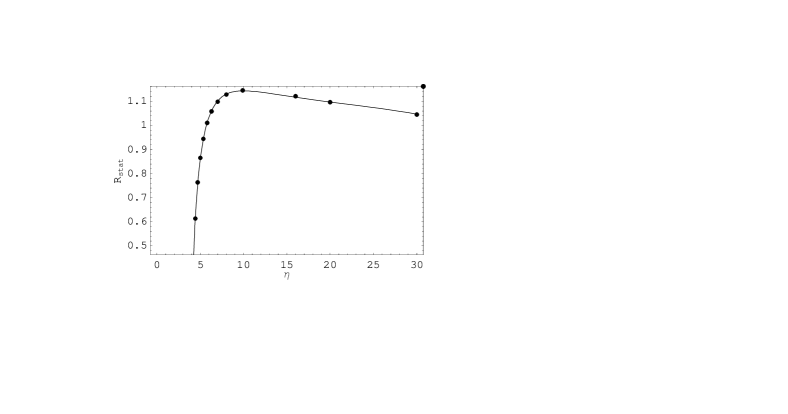
FIG. 1.: Variation of the radius (in units of $10^{6}cm$) of the static strange star as a function of the parameter $\eta$. The solid curve represents the values of the radius calculated with equation (71),while the points represent the values of the radius of the quark star obtained by numerically integrating the general relativistic structure equations of the star.

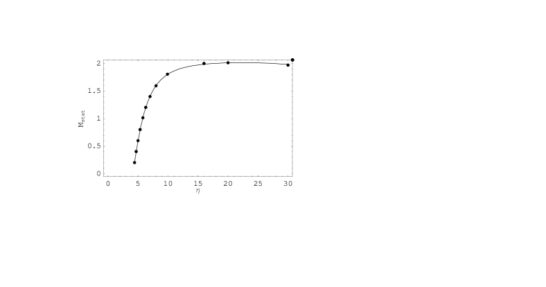
FIG. 2.: Variation of the mass of the static strange star(in solar mass units) as a function of the parameter $\eta$.The solid curve represents the values of the mass calculated with equation (72), while the points represent the values of the mass of the strange star obtained by numerically integrating the general relativistic structure equations of the star.

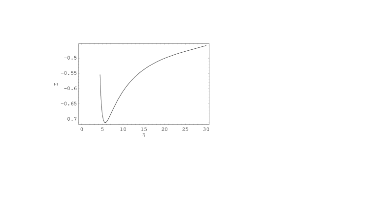
FIG. 3.: Variation of the total energy (matter+gravitational) of the static strange quark star.

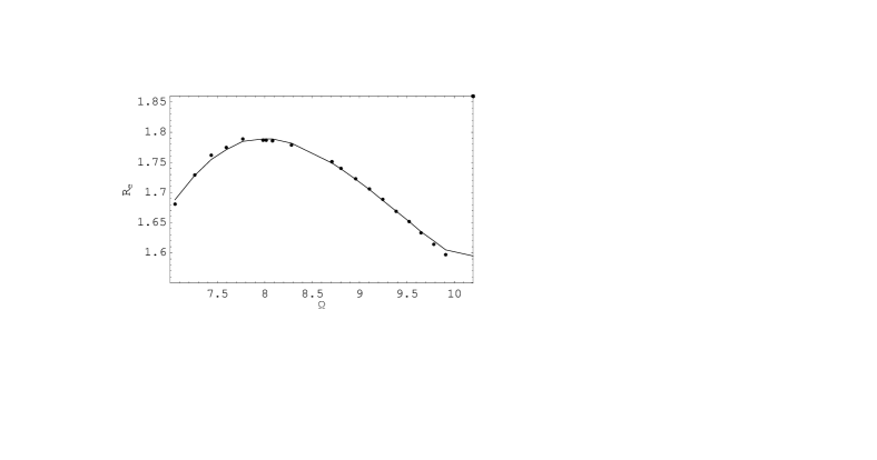
FIG. 4.: The radius of rotating strange star (in units of $10^{6}cm$) ,as a function of the angular velocity, for values of the central density in the range $\eta\in[5,16.63]$.Values obtained from the analytical expression (solid curve) are compared with data obtained by Stergioulas et al. [42] numerically integrating the gravitational field equations (points).

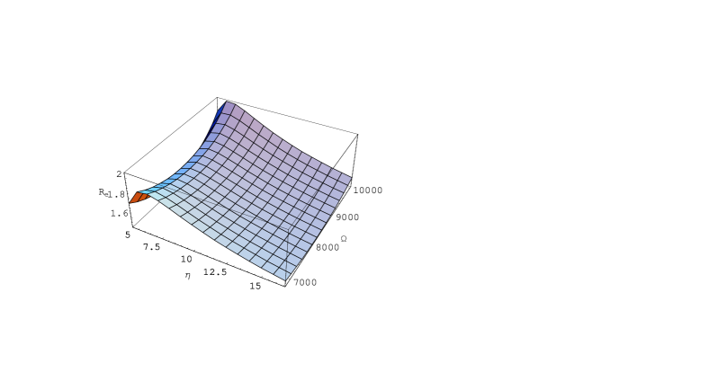
FIG. 5.: Variation of the radius of the rotating strange star (in units of $10^{6}cm$) as a function of the angular velocity $\Omega(s^{-1}$ and of the central density $\eta$.

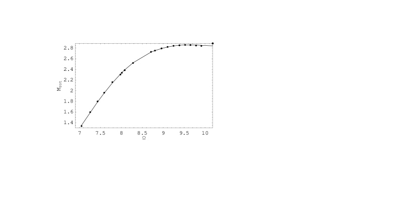
FIG. 6.: The mass of rotating strange star,expressed in solar mass units,as a function of the angular velocity, for values of the central density in the range $\eta\in[5,16.63]$.Values obtained from the analytical expression (solid curve) are compared with data obtained by Stergioulas et al. [42] numerically integrating the gravitational field equations (points).

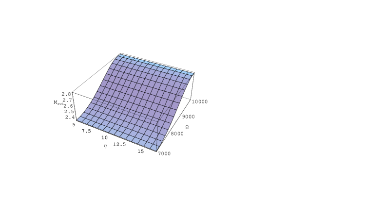
FIG. 7.: Variation of the mass of the rotating strange star,expressed in solar mass units,as a function of the angular velocity $\Omega$ and of the central density $\eta$.

REFERENCES

- [1] Kerr, R.P.,1963,Phys.Rev.Lett. 11,237.
- [2] Neugebauer, G. and Meinel, R.,1993,Astrophys.J. 414, L97.
- [3] Perjes, Z., 2000,Ann.Phys.(Leipzig) 11, 507.
- [4] Hartle, J.B., 1967, Astrophys.J. 150, 1005.
- [5] Stergioulas, N.,1998,gr-qc/9805012.
- [6] Haensel, P. and Zdunik, J.L., 1989, Nature 340,617.
- [7] Friedman, J.L., Ipser, J.R. and Parker, L.,1989, Phys.Rev.Lett.62,3015.
- [8] Haensel, P., Salgado, M. and Bonazzola, S., 1995 Astron.Astrophys. 296, 745.
- [9] Gourgoulhon, E.,Haensel, P.,Livine, R.,Paluch,E., Bonazzola, S. and Marck, J.-A.,1999, astro-ph/9907225.
- [10] Lattimer J.M., Prakash,M., Masak D. and Yahil A.,1990,ApJ 335,241.
- [11] Friedman, J.L and Ipser, J.R. 1992, Philos. Trans.R.Soc.London A340,391.
- [12] Lasota, J.-P., Haensel, P. and Abramowicz, M.A., 1996, ApJ 456,300.
- [13] Weber, F. and Glendenning, N.K., 1991, Phys.Lett.B265,1.
- [14] Weber, F. and Glendenning, N.K., 1992, ApJ bf 390,541.
- [15] Glendenning , N.K. and Weber, F. 1994, Phys.Rev. D50, 3836.
- [16] Bonazzola, S., Gourgoulhon, E., Salgado, M. and Marck, J.A. 1993, Astron.Astrophys.278, 421.
- [17] Landau, L.D. and Lifshitz, E.M., 1975, The Classical Theory of Fields, Pergamon Press, Oxford.
- [18] Adler, R., Bazin, M. and Schiffer, M, 1975, Introduction to General Relativity, New York, McGraw-Hill.
- [19] Ravenhall D.G., Pethick C.J., 1994, ApJ 424, 846.
- [20] Cook, G.B., Shapiro, S.L and Teukolsky, S.L., 1994, ApJ424,823.
- [21] Pandharipande, V.R., 1971, Nucl.Phys.A174,641.
- [22] Wiringa, R.B., Fiks, V. and Fabocini, A.,1988,Phys.Rev. bf C38,1010.
- [23] Lorenz, C.P.,Ravenhall, D.G. and Pethick, C.J.,1993,Phys.Rev.Lett.70,379.
- [24] Pandharipande, V.R., Pines, D. and Smith, R.A., 1976, ApJ208,550
- [25] Feynman, R.P.,Metropolis,N. and Teller,E.,1949,Phys.Rev.75,1561.
- [26] Baym, G.,Pethick,C. and Sutherland,P.,1971,ApJ170,299.
- [27] Witten,E.1984,Phys.Rev.D30,272.
- [28] Alcock,C.,Farhi,E. and Olinto,A. 1986, ApJ310,261.
- [29] Haensel,P.,Zdunik,J.L. and Schaeffer,R.1986 A&A160,121.
- [30] Caldwell,R.R. and Friedman,J.L. 1991,Phys.Lett.B264,143.
- [31] Cheng,K.S.,Dai,Z.G. and Lu,T. 1998,Int.J.Mod.Phys.D7,139.
- [32] Dai,Z.G.,Peng,Q.H. and Lu,T. 1995 ApJ440,815.
- [33] Cheng,K.S. and Dai,Z.G.1996,Phys.Rev.Lett.77,1210.
- [34] van den Heuvel,E.P.J. and Bitzaraki,O.1995,A&A297,L41.
- [35] Cheng,K.S. and Dai,Z.G.1998,Phys.Rev.Lett.80,18
- [36] Cheng,K.S.,Dai,Z.G.,Wei,D.M. and Lu,T.1998,Science 280,407.
- [37] Cheng,K.S. and Dai,Z.G.1998,ApJ492,281.
- [38] Dai,Z.G. and Lu,T. 1998,Phys.Rev.Lett.81,4301.
- [39] Cheng,K.S. and Dai,Z.G.1998,ApJ492,281.
- [40] Zhang,W.,Smale,A.P.,Strohmayer,T.E. and Swank,J.H.1998,ApJLett.500,L171.
- [41] Kluzniak,W.,Michelson,P. and Wagoner,R.V. 1990,ApJ358,538
- [42] Stergioulas,N.,Kluzniak,W. and Bulik,T. 1999,A&A,in press.
- [43] Farhi,E. and Jaffe,R.L. 1984,Phys.Rev.D30,2379.
- [44] Colpi,M. and Miller,J.C. 1992,ApJ388,513.
- [45] Glendenning,N.K. and Weber,F.1994,Phys.Rev.D50,3836.
- [46] Landau,L.D. and Lifshitz,E.M.1980, Statistical Physics,Pergamon Press,Oxford.
- [47] Chu,T.K.1998,MPhil Thesis of the University of Hong Kong.
- [48] Lynden-Bell,D. and Katz,J.1985 MNRAS 213,21.
- [49] Gron,O. and Johannesen,S.1992,Astrophys.Space.Sci.19,411.