Tracing the Mass during Low-Mass Star Formation. I. Submillimeter Continuum Observations
Abstract
We have obtained 850 and 450 µm continuum maps of 21 low mass cores with SED’s ranging from pre-protostellar to Class I (18K 370K), using SCUBA at the JCMT. In this paper we present the maps, radial intensity profiles, and photometry. Pre-protostellar cores do not have power-law intensity profiles, whereas the intensity profiles of Class 0 and Class I sources can be fitted with power laws over a large range of radii. A substantial number of sources have companion sources within a few arcminutes (2 out of 5 pre-protostellar cores, 9 out of 16 Class 0/I sources). The mean separation between sources is 10800 AU. The median separation is 18000 AU including sources without companions as a lower limit. The mean value of the spectral index between 450 and 850 µm is , with pre-protostellar cores having slightly lower spectral indices (). The mean mass of the sample, based on the dust emission in a 120″ aperture, is M⊙. For the sources fitted by power-law intensity distributions (), the mean value of is 1.52 0.45 for Class 0 and I sources at 850 µm and 1.44 0.25 at 450 µm. Based on a simple analysis, assuming the emission is in the Rayleigh-Jeans limit and that , these values of translate into power-law density distributions () with . However, we show that this result may be changed by more careful consideration of effects such as beam size and shape, finite outer radii, more realistic , and failure of the Rayleigh-Jeans approximation.
1 Introduction
Theories of isolated, low-mass star formation predict the distribution of density, , and dust temperature, , before and during the star formation process. These can be used to predict the spectral energy distribution (SED) and the spatial intensity distribution, , of dust continuum emission. Up to now, the primary tool for determining the evolutionary state of a particular core has been the SED, but the relationship between the SED and the distribution of matter is not unique (Butner et al. 1991, Men’shchikov & Henning 1997). Observing the spatial intensity distribution of dust continuum emission at long wavelengths, where it becomes optically thin, provides a powerful tool for constraining the actual distribution of matter (Adams 1991, Ladd et al. 1991). New instruments have recently been developed at submillimeter wavelengths that greatly enhance our capability in this area (Hunter et al. 1996, Cunningham et al. 1994). In this paper, we present maps of dust emission around 21 cores in various evolutionary states using the Submillimetre Common User Bolometer Arrray (SCUBA) (Holland et al. 1999) at wavelengths of 1.3 mm, 850µm, and 450 µm. By mapping the extended dust emission, we can probe the density structure from 7″ to 100″ (for the nearest sources in our sample, at 125 pc, these angles correspond to 870 AU to 12500 AU).
Our conception of the evolution of a dense core, first to a protostar, an object whose luminosity is dominated by accretion, then to a pre-main sequence star has been guided by an empirical evolutionary sequence (Lada 1987). Theoretical modelling of the SED (Adams, Lada, & Shu 1987) shows a good correspondence with this classification. In this scheme, sources are classified by the shape of their SED. Thus, an infrared spectral index is defined for the wavelength range =2–20m;
| (1) |
where is spectral flux density per wavelength interval. Class I sources were identified as the youngest protostars, deriving most of their luminosity from accretion. They are embedded in an envelope and have SEDs that rise () to a peak in the far-infrared. Class II and III sources are progressively less embedded than Class I sources. Class II SEDs peak in the near-infrared but possess a mid-infrared excess (), and they are normally associated with star/disk systems without a significant envelope. Class III SEDs are reddened blackbodies () and are associated with stars without optically thick disks. Class II and Class III sources typically correspond to classical and weak-line T-Tauri stars respectively.
Within the last decade, this classification scheme, which was defined in the context of infrared SEDs, has been modified to include more deeply embedded sources, which presumably represent a phase earlier than Class I. André et al. (1993) proposed the name Class 0 for sources that are so highly enshrouded that their SEDs peak longward of 100 µm and their near-infrared emission is very faint. Class 0 sources are defined to be cores which possess a central source, but which have , where is the luminosity at 350m. This criterion corresponds approximately to the mass of the centrally condensed protostellar core being less than that of the collapsing envelope. should decrease with time (André et al. 1993).
Starless cores provide plausible candidates for a still earlier stage. These starless cores are associated with dense gas cores (Myers & Benson 1983; Benson & Myers 1989) for which no source was detected by IRAS. Ward-Thompson et al. (1994) detected submillimeter emission from a sample of these objects, which they labelled “pre-protostellar cores” (PPCs, sometimes called Class sources). Pre-protostellar cores may be in hydrostatic equilibrium, or they may be gravitationally bound, magnetically sub-critical cores that are undergoing quasi-static contraction as a result of ambipolar diffusion.
In an alternative approach, Myers & Ladd (1993) defined a continuous variable, , which is the temperature of a blackbody with the same mean frequency as the observed SED. Class 0 sources have 70K while Class I sources have 70K 650K (Chen et al. 1995). has been hard to determine for pre-protostellar cores because of an absence of data at µm, but a few values are available from space-based observations in the far-infrared (Ward-Thompson, André, & Motte 1998, Ward-Thompson & André 1999).
The empirical classification scheme has been compared to theoretical models of star formation. Shu and co-workers (e.g. Shu, Adams, & Lizano 1987, Shu et al. 1993) developed a detailed theory of low mass star formation from the stage of cloud core formation to an emergent pre-main-sequence star. The simplest form of the theory (not including rotation or magnetic fields) begins with collapse inside a centrally condensed isothermal sphere ( , Shu 1977). The inside-out collapse model predicts that a wave of infall propagates outward at the sound speed of the gas. The density inside the infall radius approaches toward the center as appropriate for free fall. Core formation would then correspond to the pre-protostellar cores. Collapse would begin with the Class 0 stage and continue into the Class I stage.
This model is somewhat simplistic, and alternatives have been proposed. For instance, observational evidence exists for sharp density contrasts near the edges of cloud cores (Abergel et al. 1998). Submillimeter continuum emission from pre-protostellar cores indicates that the density distributions in the core flatten, rather than continuing to follow a single power law to small radii (Ward-Thompson et al. 1994), and line profiles consistent with infall motions have been detected in a substantial fraction of pre-protostellar cores (Lee, Myers, & Tafalla 1999, Gregersen & Evans 2000). If dynamical collapse begins before the core is fully relaxed to the isothermal sphere, there is an early stage of fast mass accretion (Basu & Mouschovias 1995, Henriksen et al. 1997), that may distinguish Class 0 from Class I sources.
Determination of the density distribution of dust in a sample including PPCs, Class 0, and Class I sources can answer some questions. Do the PPCs have density distributions predicted by theoretical models of core formation leading to inside-out collapse? Are there differences between the distributions in those with evidence for infall and those without? Are there qualitative differences in the distribution of matter around Class I sources and Class 0 sources, or is the difference only quantitative?
2 Observations
2.1 The Sample
The sample of sources (Table 1) was chosen to span a range of evolutionary states, from pre-protostellar cores to Class I sources, and to include sources with (11) and without (10) evidence of infall, based on line profile shapes in HCO+, CS, or H2CO (Gregersen et al. 1997, 2000; Gregersen and Evans 2000; Mardones et al. 1997). The coordinates were taken from a variety of references, including Ward-Thompson et al. (1994) (PPC), Gregersen et al. (1997) and Mardones et al. (1997), and corrected or updated in a few cases. Distances were obtained from a literature search, making extensive use of the compendia of Hilton & Lahulla (1995) and Lee & Myers (1999), but going back to the original references. We chose the newer, closer distances to the Ophiuchus complex ( pc) favored by de Geus et al. (1990) over the traditional choice of 160 pc, and to the Perseus clouds ( pc) according to Černis (1990) over the usual 350 pc.
Our original sample was selected to contain roughly equal numbers of PPCs, Class 0, and Class I sources. In the end, more Class 0 sources were observed, and several sources moved from Class I to Class 0 when we recalculated their properties, including our data. Changes in estimates of , , and are discussed in §3.2. We use K as the dividing line between Class I and Class 0 (Chen et al. 1995), giving us 3 Class I sources in our final sample. André et al. (1993) required for Class 0 status; with this criterion, SSV13 would be the only Class I source remaining in our sample. Consequently, we often discuss Class 0 and I sources together, referring to them as Class 0/I.
2.2 Observing and Calibration
The cores were mapped simultaneously at 850 and 450 m using SCUBA during parts of 12 nights in 1998 January, April, and May with the James Clerk Maxwell Telecsope (JCMT) on Mauna Kea, Hawaii. Nine cores were also mapped at 1.3 mm using the single bolometer detector on SCUBA. A 120″ chopper throw in azimuth was used for all the cores. Using the 64-point jiggle map mode, each SCUBA map fully samples a 23 region simultaneously at 850 and 450 m. The telescope was nodded during each map. Each jiggle map produces 4.2 minutes of integration time on the source. Because we are interested in mapping extended low brightness emission, we made 5-point maps (each a 64-point jiggle map) with a spacing of 30″. Such maps also mitigate the effects of bad bolometers. The inner 2′ of the final image was mapped in each of the 5-point maps with a total integration time of 21 minutes. The signal-to-noise ratio varied between 5 and 97 for our images (see Table 9); these estimates are conservative because the main part of the image had 5 times as much integration as the outer parts, where the noise was determined. In some cases, extra positions were observed to cover additional sources in the field.
Pointings and skydips were performed between 5-point maps. The pointing varied by less than 2″ between objects. We measured 850 and 450 during each skydip. The CSO radiometer was monitored simultaneously to obtain cso (measured at 225 GHz). Our observations confirm the correlation between this opacity and those obtained from the JCMT skydips (Chapin 1998). We used the skydips at 850 and 450 µm immediately preceding and following a 5-point map to interpolate the extinction correction. The average and standard deviation over the night in the opacities at 850 and 450 µm for each night are listed in Table 2. Opacities derived from the peak fluxes of Uranus before correction for extinction generally agreed with the opacities derived from skydips. The uncertainties in the opacity dominate the uncertainties in the total flux calibration, but they have little effect on our primary objective of imaging the sources, because the maps were obtained with a 2-D array in a short time.
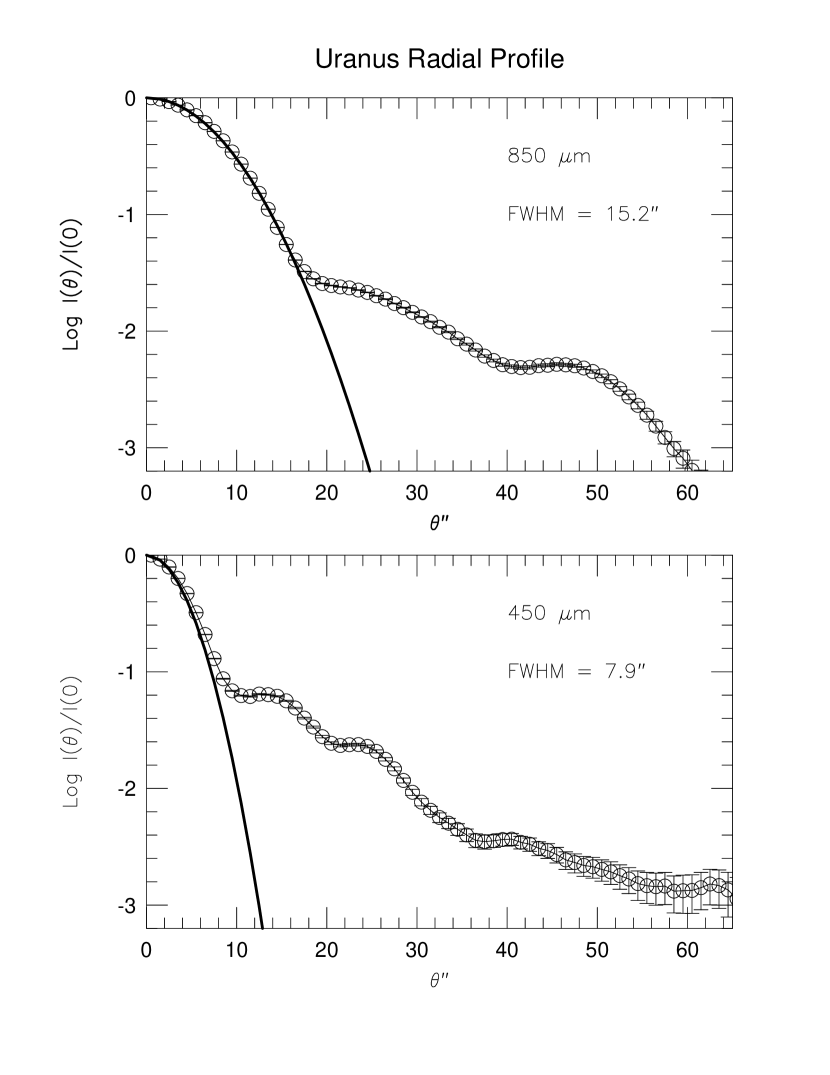
To assess the effects of image smearing when we average the components of our 5-point maps taken with different pointings, we averaged all the Uranus maps on all the runs with 1″ pixels to produce an average Uranus map. From this map, the average FWHM () at 850 and 450 µm were 152 and 79 respectively (roughly 1″ larger than values derived from a single map). Because even this worst-case experiment produced only marginal broadening, the maps are not significantly distorted by averaging data with different offsets. The average radial profiles for Uranus observed during April are shown in Figure 1 for both wavelengths; the sidelobe structure is clear and consistent with other measurements (W. Holland, personal communication). Night to night variations in the sidelobes can be seen, but amplitudes of the sidelobes vary by less than a few dB and positions of the sidelobes are roughly constant. April and August observations were made during second shift (01:30 – 09:30 HST) when the dish shape and focus had stabilized. Significant variations in sidelobe structure are seen for observations taken during first shift (17:30 – 01:30 HST) (C. Chandler personal communication). Our average 850 µm beam is characterized by sidelobes at 24″(dB) and at 47″(dB). The average 450 µm beam is characterized by sidelobes at 13″(dB), at 24″(dB), and at 40″(dB). Removing Uranus from the data makes a small change in the central Gaussian width (%) and negligible difference in the sidelobe structure (The diameter of Uranus during April 1998 was 32). We use the actual beam profile in the the modeling described in §4.2.
The total flux was calibrated using 120″ and 40″ diameter apertures in extinction corrected maps of Uranus, AFGL 618, and Mars. The observed flux densities for an aperture of diameter were computed from , where was the voltage measured at wavelength in an aperture of diameter . The calibration factors, , were calculated from the fluxes of Uranus and Mars. The total observed flux from previous SCUBA measurements was used for AFGL618 (SCUBA secondary flux calibrator webpage): Jy/beam at 850 µm; Jy/beam at 450 µm. The flux calibration did not vary substantially from night to night within an observing run but did vary from run to run. Therefore, we use an average flux calibration for each run (January, April, and August), listed in Table 2.
2.3 Image Reduction
The initial reduction of each image was performed using SURF, the SCUBA User Reduction Facility software package (Jenness & Lightfoot, 1997). The raw images of 64-point jiggle maps already have removed the effects of the chopping. The raw images are further reduced by removing the telescope nod and correcting for different bolometer gains (flat-fielding). Sky variations were subtracted by averaging the response of multiple bolometers off the source. Because some of our sources are very extended, care was taken to choose bolometers that were free of significant low level emission. After sky noise subtraction, each image was rebinned to per pixel on a B1950.0 coordinate system. SCUBA’s bolometers are subject to microphonic and 1/f noise. Excessively noisy bolometers (RMS voltage 60 nV in noise tests) were removed. Also, noisy sections of the integration were removed. These are most likely caused by imperfect subtraction of sky noise and are usually observed across several bolometers at the same time. The noisiest bolometers were typically found near the edge of the array, resulting in increased noise near the edge of the maps.
The final 5-point maps were rebinned by shifting the individual images by their centroid. Corners of the 5-point map occasionally chopped onto source emission, causing the negative beam to become visible. Bolometers in the negative beam were removed from the final image, resulting in irregularly shaped edges on many maps.
3 Results
3.1 Images
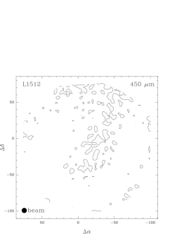
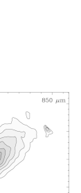
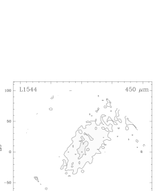
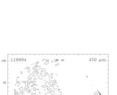
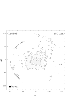
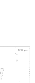
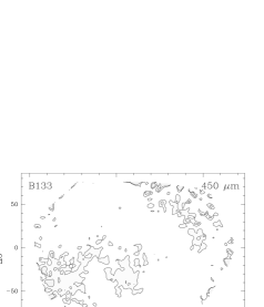
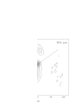
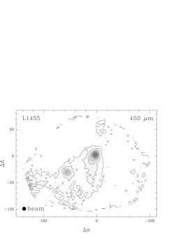
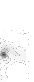
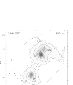
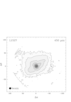
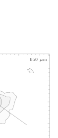
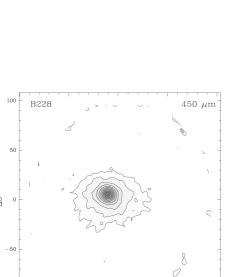
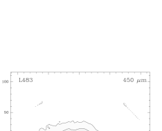
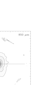
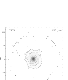
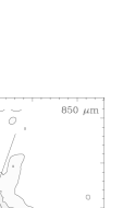
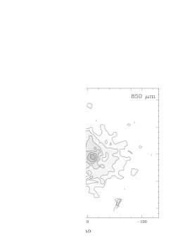
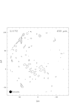
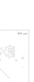
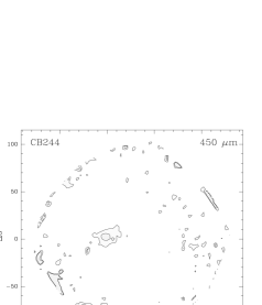
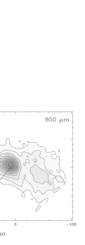
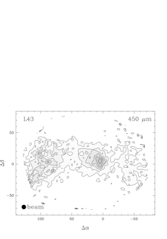
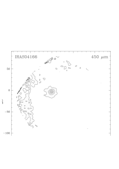
Contour plots of our SCUBA images are shown in Figures 2-8. Contour levels are indicated in each plot caption with the lowest contour . Outflow axes are marked with a solid line. The (0,0) positions are given in Table 1. Typical rms noise near the edge of the maps was 20 mJy/beam at 850µm and 100 mJy/beam at 450µm. Assuming a dust temperature of 10K near the edge of the cloud, we are sensitive to mag (1 rms) at 850µm and mag at 450µm. These correspond to column densities (H2) of cm-2 and cm-2 respectively.
Pre-protostellar cores are clearly more diffuse than the Class 0/I sources. L1512 is the most extreme in this sense, showing no evidence for a centrally peaked source. L1544 is an elongated structure with a central peak. L1689B has an elongated peak at high contour levels. However, their intensities are not as strongly peaked as the Class 0/I sources. Two out of five pre-protostellar cores have companions within 2′. L1689A has two sources visible at both wavelengths, separated by about 0.03 pc, with roughly comparable intensity. B133 has a weaker companion to the southeast. L1689B may also have multiple peaks along the east-west ridge. The maps of L1544, B133, and L1689B are consistent with maps of 1.3 mm emission toward those sources (Ward-Thompson et al. 1999; André et al. 1996).
While the pre-protostellar cores are diffuse, the Class 0/I sources are strongly centrally peaked. All the Class 0 sources except L1172 and L1455 have one well-defined centroid. B335 and B228 appear to be quite circularly symmetric, but B335 has a slight extension to the south-east visible in the 450 µm map (cf. Huard et al. 1999) that may be associated with the outflow (Bontemps et al. 1996). The other Class 0 sources all have non-spherical extensions. These extensions correspond roughly to the outflow directions in L1527, L1157, and L1455. L1157 is a particularly good example with a sizable extension to the south along the outflow axis. Other sources (L483 and IRAS03282+3035) are extended perpendicular to the outflow direction. SSV13 is elongated perpendicular to the outflow direction at high contours, but the lower contours lie along the outflow axis. It is possible that extensions along outflow directions are caused by heating of dust by short wavelength radiation escaping along the outflow cavity, while extensions perpendicular to the outflow direction reflect the distribution of maximum column density, which most models predict to be perpendicular to the outflows. This subject will be analyzed in later papers, where two-dimensional dust radiative transport can be modeled.
Nine of our sixteen Class 0/I sources have a secondary source within 2′. The L1448 cloud (L1448NW, N, and C) and SSV13 complex were known to contain multiple sources. In addition, the eastern source in L43 is seen in both the 450 µm map of Bence et al. (1998) and the 1.3 mm map of Ward-Thompson et al. (1999). We are not aware of previous detections of the additional sources toward CB244 and L1455 (see Table 3). L1455 is an extreme case with 5 sources within the SCUBA map, only one of which corresponds to a known source in this region. Continuum emission is observed to bridge between sources, making it difficult to disentangle the envelope density structure. L1172 has at least 2 peaks within a 20″ region. For the seven Class 0/I sources without secondary sources, the lack of contamination coupled with high signal-to-noise (Table 9) will allow radial intensity profiles extending up to 11 beams (at 450 µm) from the central source (see section 3.3).
For cores with more than one source, the mean separation in the plane of the sky is 10800 AU, less than twice the fragmentation scale of 6000 AU found in the Ophiuchi cores by Motte et al. (1998). A mean separation of AU is also close to the break in the distribution of optical binaries in Taurus, which Larson (1995) associates with the Jeans length, and to the length scale inferred for dynamical collapse based on specific angular momentum arguments (Ohashi et al. 1997). Looney, Mundy, & Welch (2000) find evidence for multiplicity on still smaller scales in L1448 and SSV13. They describe sources separated by AU as “separate envelope” multiplicity, and our data are consistent with this picture. The median separation, including the map size as a lower limit for sources with no detected companion, is 18000 AU.
3.2 Photometry, Classification, Spectral Index and Masses
The photometry is presented in Table 3, including calibration uncertainties. Fluxes are reported in 120″ and 40″ apertures at 1.3 mm, 850 µm, and 450 µm. Uncertainties reported include statistical uncertainties and calibration uncertainties calculated from
| (2) |
where is the flux density (Jy) and is the calibration factor (Jy/V). The uncertainties are and , the standard deviation over the run in and over the night in (Table 2) and is the mean zenith angle of the observations of the source. Photometry is presented for each source in the map that is sufficiently strong and well-defined. The offsets of the centroids from previous infrared/submillimeter positions (Table 1) are reported in Table 3.
The spectral index , defined by
| (3) |
is given in Table 4 for both 40″ and 120″ photometry, when available. Note that this definition differs from that in equation 1. The uncertainties include calibration uncertainty, which usually dominates. The values for the two aperture sizes do not differ significantly; we use the values for a 40″ aperture in the following discussion because more data are available. The mean spectral index for the collapse candidates is indistinguishable from that of sources with no evidence of collapse. The mean for the pre-protostellar cores () is slightly less than that for Class 0 and I sources (). A lower spectral index may be an indication of lower in pre-protostellar cores, resulting in failure of the Rayleigh-Jeans approximation (see §4.2). Because the difference is not statistically significant, we also calculated the mean and standard deviation of all the measurements (). If the emission were in the Rayleigh-Jeans limit, this result would imply that that between 450 and 850 µm, but this exponent should be interpreted as a lower limit if the Rayleigh-Jeans approximation fails. The average spectral index between 850µm and 1.3mm, defined in the same manner as in equation 3, is . A higher would be expected if the Rayleigh-Jeans approximation were failing at 450 µm.
Values of , , and , where includes all flux at µm, were newly computed (Table 8), including archival data and the results of our photometry. We include the archival data and references in Tables 5-7. For isolated sources, we chose data in the largest available apertures at long wavelengths, because our data show that much of the flux density comes from very extended regions. Two different methods were used to integrate the data. The uncertainties reflect uncertainties in the photometry and differences in the method of integration, but the uncertainties in do not include uncertainties in distance, since these are unavailable for many sources. Among the pre-protostellar cores, only L1544 and L1689B have the requisite far-infrared data. The of L1544 is comparable to some Class 0 sources, but the origin of the relatively strong far-infrared emission is unclear.
Some sources changed classification as a result of our data or analysis. The position of IRAS04166+2706 is close to the IRAS position, but clearly displaced from the position in Mardones et al. (1997). We calculate a lower , but the source remains a Class I source. L1448N is clearly a Class 0 source with our photometry, whereas it was borderline for Mardones et al. (who referred to it as ). The situation is similar for L1455. We find a very low for IRAS03282+3035, consistent with the upper limit of Mardones et al. (1997). For L1527 and CB244, we excluded the near-infrared data, which is clearly displaced from the submillimeter source, leading to a lower than previous estimates (Chen et al. 1995, Mardones et al. 1997). Our value of for B335 is 28 K, rather than the 37 K of Mardones et al. (1997), presumably because we include the larger flux densities that we find. Adding data at submillimeter wavelengths also decreased for L1157 and L1172, moving the latter source to Class 0. The values of for SSV13 and L43 include near-infrared data, because the emission peaks on the submillimeter position. However, SSV13 has varied substantially and depends on the epoch; we used pre-flare near-infrared data (Harvey et al. 1998). The emission in L43 (RNO91) is polarized, hence scattered. If we exclude the near-infrared data, would be , still a Class I source.
We have estimated the masses (gas and dust) from the dust emission and the equation
| (4) |
where is the flux density at 850 µm in a 120″ beam (Table 8), is the Planck function, is the opacity per gm of gas and dust at 850 µm, and we have assumed optically thin emission in a constant density sphere. The values in Table 8 were computed assuming cm2 gm-1 and K. Masses computed with K are a factor of 3.3 higher. Estimates of vary by at least a factor of 3. We have used the value for agglomerated grains with thin ice mantles (col. 5 of Table 1 of Ossenkopf & Henning 1994, hereafter OH5 dust), a model which has reproduced other data well (van der Tak et al. 1999, 2000). For comparison, we also computed the virial mass in the same (60″) radius using the width of the line most likely to be optically thin (see references in Table 8). Both calculations assumed a uniform density cloud (no temperature or density gradients). The virial mass estimate would be decreased by a factor of 0.6 in a cloud with for example. Given the uncertainties in each calculation, the agreement is good. The mean and standard deviation of the ratio are . This result is consistent (within reasonable uncertainties in and distance) with the assumption that the sources are gravitationally bound, but the uncertainties make this assumption hard to test conclusively. The mean mass is M⊙.
3.3 Radial Profiles
To compute the average intensity distribution, we assume azimuthal symmetry. While many images are not circular, experiments with taking cuts along different axes, cutting out sectors with elongated emission, etc. indicate that the overall results are not significantly affected by deviations from azimuthal symmetry. Chandler & Richer (2000) modeled the effects of outflow cavities and found that the resulting intensity profile has only a slightly lower value of .
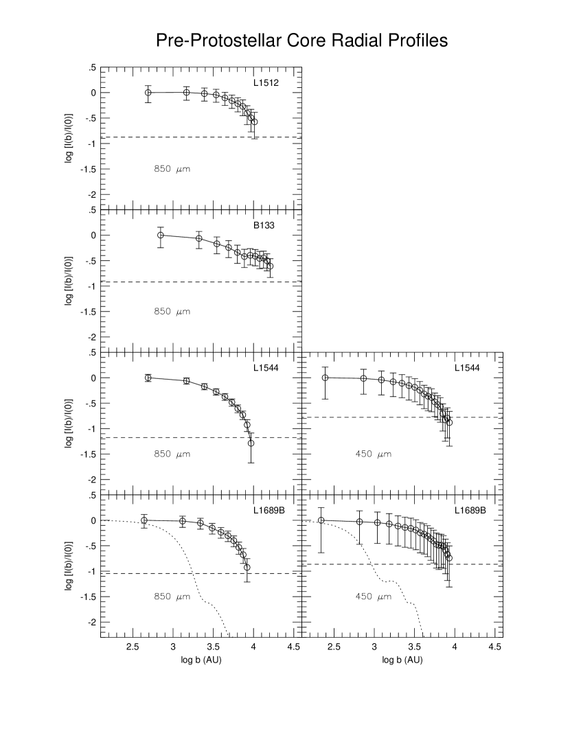
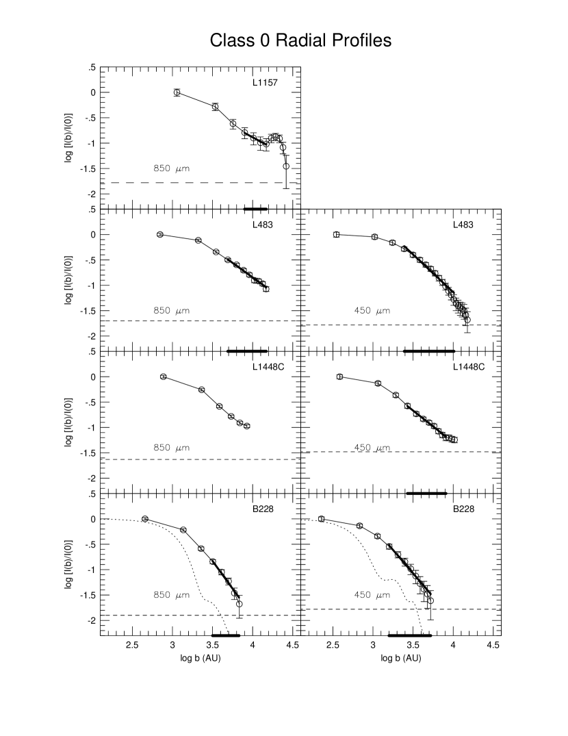
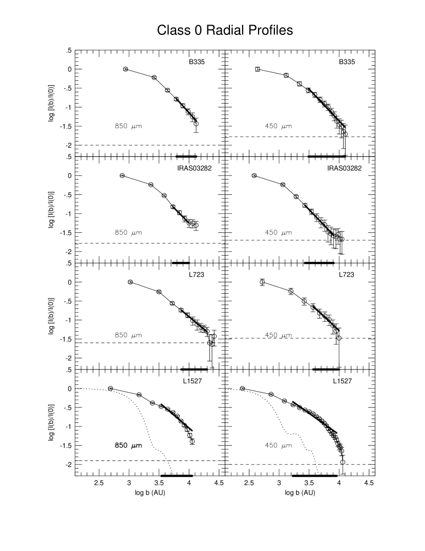
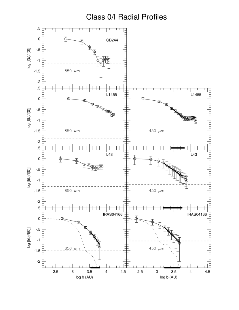
Normalized, azimuthally averaged radial profiles were made for each SCUBA image. Each image was rebinned to spacing. The mean in an annulus about impact parameter was computed from the intensity map, weighted by , where represents the area of the th pixel intercepted by the annulus and is the uncertainty in the map intensity in the th pixel. The error bars were calculated by propagating the uncertainties from the map. The radial profiles were normalized to the peak emission, and we plot . The image centroids in Table 3 were used for the center of the radial profile. To avoid effects of chopping, we terminated the radial profiles at 98″ from the centroid; points are binned at spacing (7″ at 850 m and 35 at 450 m). We have used the distances in Table 1 to convert angles to impact parameters () in units of AU. In Figs. 9–12, the normalized radial profiles () are plotted versus . The inflections in some profiles at large radii are due to contamination by secondary sources. The point-to-point fluctuations in the profile are substantially less than the errorbars because half-beam sampling was used. The radial profiles agree well with those of 1.3 mm emission presented by André et al. (1996) and Ward-Thompson et al. (1999). The radial intensity profiles of L1448-C agree well with those of Chandler & Richer (2000), but our profile of L1527 is steeper than those found by either Chandler & Richer (2000) or Hogerheijde & Sandell (2000).
Previous observations of pre-protostellar cores showed that the radial intensity profile did not follow a single power law, but a broken power law was able to fit the limited data (Ward-Thompson et al. 1994). Maps of millimeter emission (Ward-Thompson, Motte, & André 1999) have clearly shown the flattening of in the inner regions. While the outer regions can be approximated by a power law, André et al. (1996) commented that the north-south cut through L1689B would be described better by a Gaussian than by a power law. It is clear from Figure 9 that a power-law does not fit any portion of the pre-protostellar core radial intensity profiles in the submillimeter, confirming the result of Ward-Thompson et al. (1999). Our results for pre-protostellar cores are consistent with observations of a larger sample (André et al. 2000).
Models of core formation leading to inside-out collapse predict a flat inner core approaching at larger radii, and the flat core should shrink toward the center with time. While our observations do not appear to be consistent with these models, we caution that detailed modeling is still needed. If the evidence for large-scale infall in all of these cores but L1512 (Lee, Myers, & Tafalla 1999; Gregersen & Evans 2000) is correct, then infall may begin before the core has fully relaxed to a singular isothermal sphere with (e.g., Shu 1977).
In contrast, the intensity profiles of most Class 0/I sources (Figures 10–12) can be fitted with power laws, if the inner three points, which are affected by the finite beam size, and the outermost points (noisy, and possibly affected by the finite chop size or other sources) are ignored. Power law fits (, with corresponding to ) were made to 8 cores at 850 m and 10 cores at 450 m. The uncertainty in the value of (Table 9) includes the deviations from a straight line and the standard deviation from the radial profiles, as described above. Fits used only points in the profile where the signal was greater than the noise in each bin. Fits for images with multiple sources are terminated at the intensity minimum between the sources. The slopes () from these fits are tabulated in Table 9. The average slopes are at 850 µm and at 450 µm for Class 0/I sources. Since the values of determined at different wavelengths agree well, we average all values to obtain . The average slope for Class I sources does not differ significantly from that for Class 0 sources, but a larger sample of Class I sources is needed. We are unable to distinguish statistically significant differences in the average slope between sources with () and without () evidence for collapse.
4 Analysis
4.1 Density Distributions: A Simple Analysis
Combining the value of the slopes in the radial intensity profiles with a knowledge of the temperature distribution of dust grains, , constrains the density distribution of dust grains, . If the emission is optically thin and the opacity () of the dust grains does not vary with radius, the observed intensity at an impact parameter, , is given by
| (5) |
(Adams 1991), where is the outer radius. If we assume power law distributions for the density and temperature,
| (6) |
| (7) |
) where is a fiducial radius, then, if the emission is in the Rayleigh-Jeans limit and if , equation (5) simplifies to
| (8) |
The dust opacity for grains in the submillimeter portion of the spectrum roughly follows a power law (see Ossenkopf & Henning 1994). Using this assumption the temperature distribution around a centrally heated source follows a power law of the form
| (9) |
(cf. Doty & Leung 1994). Estimates of typically vary between 0 to 2 in the submillimeter. For , consistent with our data (§3.2), . In this case, , and the found above translates into for Class 0/I sources. For the slope of the density power law changes slightly to . These values are consistent with those found by Chandler & Richer (2000), with the exception of L1527 (see also Hogerheijde & Sandell 2000). Within the uncertainties, these values are consistent with the density distribution expected from an isothermal sphere or the outer parts of a Bonnor-Ebert sphere (Shu 1977). However, there are quite a few caveats.
4.2 Some Caveats
For sources without confusing secondary sources, the data often fall below the fit at large radii. This behavior could be attributed to an outer radius where the profile becomes steeper (e.g., Abergel et al. 1998). We are wary of this conclusion for several reasons. Some of the turn-down near the edge may be caused by using a finite chop. Since our sources have very extended envelopes, we may have chopped onto low level emission, decreasing the observed emission. While we tried to avoid this effect by only carrying the radial profiles out to 98″, it still may be a problem.
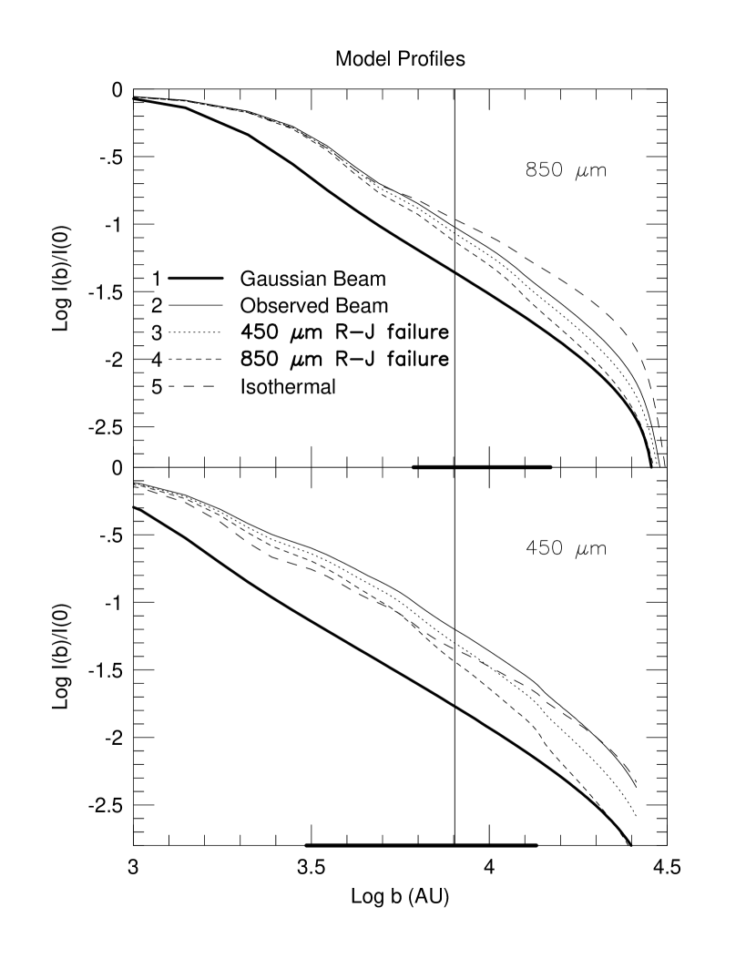
To investigate the importance of various effects on the radial profiles, we constructed 5 spherically symmetric models (Fig. 13). All 5 models calculate the observed intensity, generalizing equation 5 to allow finite optical depth, and convolve the result with a beam profile; they use a code generously supplied by L. Mundy. We assumed power laws for and ( and ) and use OH5 opacities for coagulated dust grains with icy mantles (Ossenkopf & Henning 1994). The source was placed at a distance of 200 pc with a total mass of 1.1 M⊙, equal to the mean distance ( pc) and mean mass of the sample. An inner radius for the dust shell of 60 AU and an outer radius of 30000 AU (corresponding to 024 and 120″) were used. Model 1 assumes gaussian beams with the FWHMs of 152 and 79 at 850µm and 450µm respectively. Models 2 – 5 have been convolved with our observed beam profiles. The sidelobes clearly increase the normalized intensity throughout the profile and spread the effects of a finite outer radius back to smaller impact parameters. If very small and very large impact parameters are excluded from the fit, the effect on the fitted slope is small ().
Another important issue is Rayleigh-Jeans failure in equation 5, which occurs when the dust temperature falls below ( = 32 K and 17 K at 450 and 850 µm, respectively). This is a problem for the emission at large distances from the low luminosity, highly embedded sources that we are observing because the dust temperature does drop below . Model 2 in Fig. 13 shows the observed intensity profile for a source in which over the entire profile. Models 3 and 4 use the same but were normalized to lower temperatures, such that dropped below at 450 µm (model 3) and 850 µm (model 4) at 8000 AU. Rayleigh-Jeans failure results in an increase in by as much as 0.5, leading to an overestimate of by the same amount.
The temperature is only approximated by a power-law (eq. 7). The actual is probably steeper in the inner regions, where the radiative transfer of heating radiation is optically thick (e.g., Doty & Leung 1994). More importantly for this analysis, if the core is exposed to the interstellar radiation field, can flatten out or even rise again in the outer regions. Figure 13 also shows model 5 in which the temperature distribution is isothermal () from 3000 AU outward. A flattening of causes a decrease in by as much as 0.5. The typical interstellar radiation field is capable of heating dust to about 14 K at the extinctions probed by submillimeter emission. This slight rise would be expected to cause a further decrease in . Consequently, uncertainties of about are present in deducing the value of from simple fits assuming power-laws for temperature and the Rayleigh-Jeans approximation. To correct for these effects, careful modeling of each source is needed. These models will be the subject of a later paper.
Although we have assumed spherical symmetry in the previous analysis, the actual geometry of these cores is certainly much more complex. Elongated extensions at low contour levels are seen in many sources. The slope of the intensity profile is not greatly affected by these extensions. The at 850 and 450 µm was modified by 0.1 when sectors containing the extensions were eliminated from the azimuthal average. This appears to be a small correction compared to other uncertainties in the analysis.
We have also assumed that is constant throughout the radial profile. Ambipolar diffusion can cause a relative drift between the gas and the dust and between the different dust grain populations. The former may lead to spatial variations in the dust-to-gas ratio, and the latter will also cause to vary across the cores. Substantial molecular depletions and grain aggregations in the central regions of some cores can also lead to changes in . Visser et al. (1998) interpreted decreases in spectral index toward column density peaks in NGC 2024 in terms of a decrease in in dense cores, possibly caused by grain growth. The correction factor to for Rayleigh-Jeans failure is
| (10) |
where the spectral index is given by (Visser et al. 1998). If we assume , then . Applying this correction increases the estimate of from 0.8 found in §3.2 to 1.5 for the data in a 40″ aperture. The Rayleigh-Jeans correction factor varies quickly at low temperatures. For example, changes by 0.5 between 10 and 14 K, plausible changes in from the center to edge of an externally heated pre-protostellar core. Chandler & Richer (2000) saw little evidence for changes in with radius, but Hogerheijde & Sandell (2000) did observe changes in a few cases.
5 Conclusions
The main conclusions of our study are as follows.
Pre-protostellar cores are clearly more diffuse that Class 0/I sources. Pre-protostellar cores do not have central peaks that are as well defined as those in Class 0/I sources. Many sources had companion sources within 2′ (2/5 pre-protostellar core, 9/16 Class 0/I sources). The presence of several sources in an IRAS beam means that previous studies of SEDs may have been distorted. Observations with higher spatial resolution in the far-infrared are needed. For the sources with companions, the mean projected separation is 10,800 AU, more than the mean separation of 6000 AU in the Ophuichi cluster (Motte et al. 1998), and close to radii previously suggested to be significant for setting the scale for star formation (Larson 1995, Ohashi et al. 1997). The median separation is 18000 AU including lower limits for sources with no detected companions. These results suggests that truly isolated star formation is uncommon.
Some Class 0/I sources show extensions, sometimes along the outflow axis and sometimes perpendicular to it. Both heating and column density effects may play a role in defining the shapes at low contour levels.
The mean spectral index for all sources between 450 and 850 µm is . This value would imply an exponent in the opacity law, , but Rayleigh-Jeans failure could increase this value. Pre-protostellar cores have a slightly lower average spectral index (). The average spectral index measured at 850µm and 1.3mm is higher ().
The mean mass in the sample is . The masses computed from the dust emission agree reasonably with those computed from the virial theorem, supporting the hypothesis that the cores are gravitationally bound and that the values used for the dust opacity are reasonable.
The radial intensity profiles of pre-protostellar cores cannot be fitted with power laws over a significant range of radii. In contrast, most Class 0/I sources can be fitted with power laws if the inner and outer points are excluded. For some sources, the fit must be truncated before emission from secondary sources affects the profile. The mean slope is for Class 0/I sources. We are unable to distinguish between Class 0 and Class I radial profiles with our limited sample. A simple analysis suggests that a density power law , with would fit the data.
Models that include more accurate , account for Rayleigh-Jeans failure, and include the actual beam shape show that the simple analysis can be misleading. These models still can be fitted by power laws in the normalized intensity, but the fitted slope may vary by compared to the simple analysis.
Given the likely complexities in real cores, it is somewhat surprising that simple power-law models fit the Class 0/I sources as well as they do. Neither the mean spectral indices nor the slopes in the intensity profiles distinguish between Class 0 and Class I sources nor between candidates and non-candidates for collapse in the present sample. Firmer conclusions await a larger sample of Class I sources and detailed, source-by-source modeling.
Acknowledgments
We are grateful to T. Jenness for assistance with SURF, to L. Mundy for providing the computer code used to generate the models in Figure 13, and to the staff of the JCMT for crucial support while observing. We thank Claire Chandler and the referee for comments that improved the paper. The JCMT is operated by the Joint Astronomy Centre on behalf of the Particle Physics and Astronomy Research Council of the United Kingdom, The Netherlands Organization for Scientific Research and the National Research Council of Canada. We thank the State of Texas and NASA (Grant NAG5-7203) for support. NJE thanks the Fulbright Program and PPARC for support while at University College London and NWO and NOVA for support in Leiden.
References
- (1)
- (2) Abergel, J. P. B., et al. 1998, in ASP vol. 132, Star Formation with the Infrared Space Observatory, ed. J. L. Yun & R. Liseau (Provo:BYU), 220
- (3) Adams, F. C., Lada, C. J., & Shu, F. H. 1987, ApJ, 312, 788
- (4) Adams, F. C. 1991, ApJ, 382, 544
- (5) André, P., Ward-Thompson, D., & Barsony, M. 1993, ApJ, 406, 122
- (6) André, P., Ward-Thompson, D., & Motte, F. 1996, A&A, 314, 625
- (7) André, P., Ward-Thompson, D., & Barsony, M. 2000, In Protostars and Planets IV, ed. V. Mannings, A. Boss, S. Russell. (Tucson:Univ. Arizona), in press.
- (8) Aspin, C., Sandell, G. 1994, A&A, 288, 803
- (9) Bachiller, R., Martin-Pintado, J., Tafalla, M., Cernicharo, J., & Lazareff, B. 1990, A&A, 231, 174
- (10) Bachiller, R., André, P., & Cabrit, S. 1991b, A&A, 214, L43
- (11) Bachiller, R., Martin-Pintado, J., & Planesas, P. 1991a, A&A, 251, 639
- (12) Bachiller, R., Terebey, S., Jarret, T., Martin-Pintado, J., Beichman, C., & van Buren, D. 1994, ApJ, 437, 296
- (13) Bachiller, R., Guilloteau, S., Dutrey, A., Planesas, P., & Martin-Pintado, J. 1995 A&A, 299, 857
- (14) Bachiller, R., & Perez Gutierrez, M. 1997, ApJ, 487, L93
- (15) Barsony, M., Ward-Thompson, D., André, P., & O’Linger, J. 1998, ApJ, 509, 733
- (16) Basu, S. & Mouschovias, T. Ch. 1995, ApJ, 453, 271
- (17) Bence, S. J., Padman, R., Isaak, K. G., Wiedner, M. C., & Wright, G. S. 1998, MNRAS, 299, 965
- (18) Benson, P. J., & Myers, P. C. 1989, ApJS, 71, 89
- (19) Benson, P. J., Caselli, P. & Myers, P. C. 1998, ApJ, 506, 743
- (20) Bontemps, S., Andre, P., Terebey, S. & Cabrit, S. 1996, A&A, 311, 858
- (21) Butner, H. M., Evans N. J. II, Lester, D. F., Levreault, R. M., Strom, S. E. 1991, ApJ 376, 636.
- (22) Černis, K. 1990, Ap&SS, 166, 315
- (23) Chandler, C. J., & Richer, J. S. 2000, ApJ, in press (astro-ph/9909494)
- (24) Chapin, E. 1998, Submillimetre Sky Opacity Calibration at the James Clerk Maxwell Telescope, Physics Co-op Work Term Report
- (25) Chen, H. Myers, P. C., Ladd, E. F., & Wood, D. O. S. 1995, ApJ, 445,377
- (26) Cunningham, C. R., Gear, W. K., Duncan, W. D., Hastings, P. R., Holland, W. S. 1994, Proc. SPIE 2198, 638
- (27) Dame, T. M., & Thaddeus, P. 1985, ApJ, 297, 751
- (28) Davidson, J. A., & Jaffe, D. T. 1984, ApJ, 277, L13
- (29) Davidson, J. A. 1987, ApJ, 315, 602
- (30) de Geus, E., Bronfman, L., & Thaddeus, P. 1990, A&A, 231, 137
- (31) Doty, S. D., & Leung C. M. 1994, ApJ, 424, 729
- (32) Elias, J. 1978, ApJ, 224, 453
- (33) Fuller G. A., Lada, E. A., Masson, C. R., & Myers, P. C. 1995, 453, 754
- (34) Gee, G., Griffin, M. J., Cunningham, T., Emerson, J. P., Ade, P. A. R., & Caroff, L. J., 1985, MNRAS, 215, 15
- (35) Goldsmith, P. F., Snell, R. L., Hemeon-Heyer, M., Langer, W. D. 1984, ApJ, 286, 599
- (36) Gregersen, E. M. 1998, PhD Dissertation, The University of Texas at Austin
- (37) Gregersen, E. M., & Evans, N. J., II 2000, ApJ, in press
- (38) Gregersen, E. M., Evans, N. J., II, Zhou, S., & Choi, M. 1997, ApJ, 484, 256
- (39) Gregersen, E. M., Evans, N. J., Mardones, D. M., & Myers, P. C. 2000 ApJ, in press (astro-ph/9912175)
- (40) Gueth, F., Guilloteau, S., Dutrey, A., Bachiller, R. 1997, A&A, 323, 943
- (41) Harvey, P. M., Smith, B. J., Di Francesco, J., & Colome, C. 1998, ApJ, 499, 294
- (42) Henriksen, R., André, P., & Bontemps, S. 1997, A & A, 323, 549
- (43) Herbig, G. H., & Jones, B. F. 1983, AJ, 88, 1040
- (44) Heyer, M. H., & Graham, J. A. 1989, PASP, 101, 816
- (45) Hilton, J. & Lahulla, J. F. 1995, A&AS, 113, 325
- (46) Hirano, N., Hayashi, S. S., Umemoto, T., & Ukita, N. 1998, ApJ, 504, 334
- (47) Hogerheijde, M. R., & Sandell, G. 2000, ApJ, in press (astro-ph/0001021)
- (48) Holland et al. 1999, MNRAS 303, 659
- (49) Huard, T. L., Sandell, G. & Weintraub, D. A. 1999, ApJ, 526, 833
- (50) Hunter, T. R., Benford, D. J., Serabyn, E. 1996, PASP 108, 1042
- (51) Jenness, T., & Lightfoot, J.F. 1997, SURF - SCUBA User Reduction Facility ver. 1.1 User’s Manual
- (52) Keene, J., et al. 1983, ApJ, 274, L43
- (53) Kenyon, S., Hartmann, L., Strom, K., Strom, S. 1990, ApJ, 99, 869
- (54) Lada, C. J. 1987, in IAU Symp. 115, Star Formation Regions, ed. M Peimbert & J. Jugaku (Dordrecht:Reidel), 1
- (55) Ladd, E. F., et al. 1991, ApJ, 366, L203
- (56) Larson, R. B. 1995, MNRAS, 272, 213
- (57) Larsson, B. 1998, ASP Conf. Ser. 132: Star Formation with the Infrared Space Observatory, ed. J. L. Yun & R. Liseau (Provo:BYU), 382
- (58) Launhardt, R., & Henning, Th. 1997, A&A, 326, 329
- (59) Lee, C. W., & Myers, P. C. 1999, ApJS, 123, 233
- (60) Lee, C. W., Myers, P. C.,& Tafalla, M. 1999, ApJ, 526, 788
- (61) Liseau, R., Sandell, G., & Knee, L. B. G. 1988, A&A, 192, 153
- (62) Looney, L. W., Mundy, L. G., & Welch, W. J. 2000, ApJ, in press (astro-ph/9908301)
- (63) Mardones, D., Myers, P. C., Tafalla, M., Wilner, D. J., Bachiller, R., & Garay, G. 1997, ApJ, 489, 719
- (64) Men’shchikov A. B., & Henning, Th. 1997, A&A 318, 879
- (65) Motte, F. André, P., & Neri, R. 1998, A&A 336, 150
- (66) Murphy, D. C., Cohen, R., & May, J. 1986, A&A, 167, 234
- (67) Myers, P. C., & Benson, P. J. 1983, ApJ, 266 309
- (68) Myers, P. C., Fuller, G. A., Mathieu, R. D., Beichman, C. A., Benson, P. J., Schild, R. E., & Emerson, J. P. 1987, ApJ, 319, 340
- (69) Myers, P. C., & Ladd, E. F. 1993, ApJ, 413, L47
- (70) Ohashi, N., Hayashi, M., Ho, P. T. P., Momose, M., Tamura, M., Hirano, N., & Sargent, A. I. 1997, ApJ, 488, 317
- (71) Ossenkopf, V., & Henning, Th. 1994, A & A, 291, 943
- (72) Reipurth, B. A., Chini, R., Krugel, E., Kreysa, E., & Sievers, A. 1993, A&A, 273, 221
- (73) Shu, F. H. 1977, ApJ, 214, 488
- (74) Shu, F. H., Adams, F. C., & Lizano, S. 1987, ARA & A, 25, 23
- (75) Shu, F. , Najita, J. , Galli, D. , Ostriker, E. & Lizano, S. 1993, Protostars and Planets III, 3
- (76) Straižys, V. Černis, K., Kazlauskas, A., & Meištas, E. 1992, Baltic Astr., 1, 149
- (77) Terebey, S., Shu, F. H., & Cassen, P. 1984, ApJ, 286, 529
- (78) Tomita, Y., Saito, T., Ohtani, H. 1979, PASJ, 31, 407
- (79) van der Tak, F. F. S., van Dishoeck, E. F., Evans, N. J., II, Bakker, E. J. & Blake, G. A. 1999, ApJ, 522, 991
- (80) van der Tak, F. F. S., van Dishoeck, E. F., Evans, N. J., II, & Blake, G. A. 2000, ApJ, in press (astro-ph/0001527)
- (81) Visser, A. E., Richer, J. S., Chandler, C. J., & Padman, R. 1998, MNRAS, 301, 585
- (82) Ward-Thompson, D., & André, P. 1999, in The Universe as seen by ISO, ESA SP-427, ed. P. Cox & M. F. Kessler (Noordwijk: ESA) 463
- (83) Ward-Thompson, D., Motte, F., & André, P. 1999, MNRAS, 305, 143
- (84) Ward-Thompson, D., Scott, P. F., Hills, R. E., & André, P. 1994, MNRAS, 268, 276
- (85) Ward-Thompson, André, P. H., Motte, F., 1998, in ASP vol. 132, Star Formation with the Infrared Space Observatory, ed. J. L. Yun & R. Liseau (Provo:BYU), 195
- (86) Yun, J. L., & Clemens, D. P. 1994, ApJS, 92, 145
- (87) Zhou, S., Evans, N. J., Wang, Y. 1996, ApJ, 406, 296
- (88)


| Source | (1950.0) | (1950.0) | Observed | ClassaaPPC=Pre-protostellar core | Dist. | Dist. | Outflow | CollapsebbAs indicated by studies of HCO+ (Gregersen 1998) |
|---|---|---|---|---|---|---|---|---|
| (h m s ) | (∘ ′ ″) | (pc) | Ref. | Ref. | Candidate? | |||
| L1512 | 05 00 54.4 | 32 39 37 | 1/25/98 | PPC | 140 | 1 | … | N |
| L1544 | 05 01 13.1 | 25 06 36 | 1/25/98 | PPC | 140 | 1 | … | Y |
| L1689A | 16 29 10.5 | 24 57 22 | 4/18/98 | PPC | 125 | 2 | … | Y |
| L1689B | 16 31 47 | 24 31 45 | 4/18/98 | PPC | 125 | 2 | … | Y |
| B133 | 19 03 27.3 | 06 57 00 | 4/14/98 | PPC | 200 | 3 | … | Y |
| L1448NW | 03 22 31.1 | 30 35 04 | 1/24/98 | 0 | 220 | 4 | 10,11 | N |
| L1448N | 03 22 31.8 | 30 34 45 | 1/24/98 | 0 | 220 | 4 | 10,11 | N |
| L1448C | 03 22 34.3 | 30 33 30 | 1/24/98 | 0 | 220 | 4 | 10,11 | N |
| L1455 | 03 24 34.9 | 30 02 36 | 1/24/98 | 0 | 220 | 4 | 6 | N |
| IRAS03282+3035 | 03 28 15.2 | 30 35 14 | 1/24/98 | 0 | 220 | 4 | 12 | Y |
| L1527 | 04 36 49.6 | 25 57 21 | 1/25/98 | 0 | 140 | 1 | 13 | Y |
| B228 | 15 39 50.4 | 33 59 42 | 4/15/98 | 0 | 130 | 5 | 14 | Y |
| L483 | 18 14 50.6 | 04 40 49 | 4/17/98 | 0 | 200 | 3 | 15 | NccRed asymmetry in HCO+, but blue in other lines |
| L723 | 19 15 41.3 | 19 06 47 | 4/20/98 | 0 | 300 | 6 | 16 | N |
| B335 | 19 34 35.4 | 07 27 24 | 4/17/98 | 0 | 250 | 7 | 16 | Y |
| L1157 | 20 38 39.6 | 67 51 33 | 4/19/98 | 0 | 325 | 8 | 17 | Y |
| L1172 | 21 01 44.2 | 67 42 24 | 4/18/98 | 0 | 288 | 8 | … | N |
| CB244 | 23 23 48.7 | 74 01 08 | 4/20/98 | 0 | 180 | 9 | 18 | Y |
| SSV13 | 03 25 57.9 | 31 05 50 | 1/24/98 | I | 220 | 4 | 19 | N |
| IRAS04166+2706 | 04 16 37.8 | 27 06 29 | 8/30/98 | I | 140 | 1 | … | Y |
| L43 | 16 31 37.7 | 15 40 52 | 4/17/98 | I | 125 | 2 | 20 | N |
References. — 1. Taurus – Elias 1978; 2. Ophiuchus – de Geus et al. 1990; 3. Aquila Rift – Dame & Thaddeus 1985; 4. NGC1333 region – Černis 1990, (but see Herbig & Jones 1983 who get 350 pc); 5. Lupus – Murphy et al. 1986; 6. Goldsmith et al. 1984; 7. Tomita et al. 1979; 8. Straižys et al. 1992; 9. Lindblad Ring – Launhardt & Henning 1997; 10. Bachiller et al. 1990; 11. Barsony et al. 1998; 12. Bachiller et al. 1991a; 13. Zhou et al. 1996; 14. Heyer & Graham 1989; 15. Fuller et al. 1995; 16. Hirano et al. 1998; 17. Bachiller & Perez Gutierrez 1997; 18. Yun & Clemens 1994; 19. Liseau et al. 1988; 20. Bence et al. 1998
| Date | ||||||||
|---|---|---|---|---|---|---|---|---|
| Jy/VaaCalibration Factor for a 40″ diameter aperture | Jy/VbbCalibration Factor for a 120″ diameter aperture | Jy/VaaCalibration Factor for a 40″ diameter aperture | Jy/VbbCalibration Factor for a 120″ diameter aperture | Jy/VaaCalibration Factor for a 40″ diameter aperture | ||||
| January | 1.02 (0.06) | 0.84 (0.04) | 5.72 (0.99) | 5.24 (1.97) | … | |||
| 01/24/98 | 0.17 (0.01) | 0.84 (0.01) | … | |||||
| 01/25/98 | 0.12 (0.01) | 0.48 (0.06) | … | |||||
| April | 0.94 (0.05) | 0.74 (0.04) | 5.76 (0.76) | 4.14 (0.57) | … | |||
| 04/14/98 | 0.12 (0.01) | 0.51 (0.01) | … | |||||
| 04/15/98 | 0.14 (0.01) | 0.60 (0.02) | … | |||||
| 04/17/98 | 0.14 (0.01) | 0.66 (0.06) | 0.06 (0.01) | |||||
| 04/18/98 | 0.15 (0.01) | 0.69 (0.05) | … | |||||
| 04/19/98 | 0.34 (0.03) | 1.7 (0.1) | … | |||||
| 04/20/98 | 0.15 (0.03) | 0.7 (0.2) | … | |||||
| August | 1.00 (0.05) | … | 4.63 (0.99) | … | 0.26(0.04) | |||
| 08/28/98 | 0.39 (0.01) | 2.7 (0.2) | 0.15 (0.01) | |||||
| 08/29/98 | 0.20 (0.01) | 1.2 (0.1) | … | |||||
| 08/30/98 | 0.19 (0.01) | 1.0 (0.1) | … |
| Source | Centroid | (Jy) | ||||
|---|---|---|---|---|---|---|
| (″,″) | 1.3 mmaaIn a 40″ aperture | 850 maaIn a 40″ aperture | 850 mbbIn a 120″ aperture | 450 maaIn a 40″ aperture | 450 mbbIn a 120″ aperture | |
| L1512 | (19,26) | … | 0.35(0.02) | 1.81(0.09) | 1.6(0.3) | 8.5(3.2) |
| L1544 | (1,4) | 0.27(0.04) | 1.12(0.07) | 3.64(0.18) | 4.2(0.8) | 17.4(6.7) |
| L1689A | (4,9) | … | 0.54(0.03) | … | 3.9(0.6) | … |
| (51,24) | … | 0.55(0.03) | … | 3.4(0.5) | … | |
| L1689B | (1,12) | … | 0.90(0.05) | 3.18(0.18) | 3.2(0.5) | 10.8(1.7) |
| B133 | (13,32) | … | 0.60(0.03) | 2.06(0.12) | 3.4(0.5) | 11.8(1.6) |
| L1448NW | (0,0) | … | 6.51(0.38) | … | 43.9(7.6) | … |
| L1448N | (,1) | … | 8.19(0.49) | … | 56.4(9.8) | … |
| L1448C | (0,3) | 0.74(0.11) | 3.95(0.24) | … | 31.8(5.5) | … |
| L1455 | (3,1) | … | 1.08(0.06) | … | 10.2(1.8) | … |
| (55,30) | … | 0.94(0.06) | … | 7.7(1.3) | … | |
| (9,59) | … | 0.38(0.02) | … | 2.5(0.5) | … | |
| (10,47) | … | 0.91(0.05) | … | 6.9(1.2) | … | |
| IRAS03282+3035 | (6,8) | … | 1.74(0.10) | 3.59(0.17) | 9.9(1.7) | 25.0(9.4) |
| L1527 | (2,0) | 0.72(0.11) | 3.19(0.19) | 9.41(0.46) | 18.2(3.2) | 55.5(20.9) |
| B228 | (11,5) | … | 2.63(0.15) | 4.23(0.24) | 19.6(2.7) | 25.9(3.7) |
| L483 | (1,2) | … | 3.74(0.20) | 9.25(0.51) | 30.1(4.6) | 59.2(1.7) |
| L723 | (8,1) | … | 1.79(0.11) | 3.60(0.23) | 8.5(2.1) | 12.4(3.1) |
| B335 | (0,1) | 0.57(0.09) | 2.28(0.12) | 3.91(0.22) | 14.6(2.2) | 21.1(3.3) |
| L1157 | (0,1) | 0.58(0.09) | 2.41(0.19) | 5.03(0.40) | … | … |
| L1172 | (10,2) | … | 0.66(0.04) | 2.69(0.15) | 5.2(0.8) | 16(3) |
| CB244 | (0,1) | 0.25(0.04) | 1.04(0.08) | 1.86(0.14) | 5.1(1.9) | 9.0(3.4) |
| (75,45) | … | 0.78(0.06) | … | 3.1(1.2) | … | |
| SSV13 | (1,10) | 1.83(0.28) | 6.95(0.41) | … | 52.4(9.1) | … |
| IRAS04166+2706 | (1,) | … | 1.08(0.06) | … | 4.2(1.0) | … |
| L43 | (7,5) | … | 1.60(0.09) | … | 11.8(2.0) | … |
| (89,6) | … | 1.80(0.10) | … | 11.4(1.9) | … |
| Source | Centroid | aaIn a 40″ aperture | aaIn a 40″ aperture | bbIn a 120″ aperture |
|---|---|---|---|---|
| L1512 | (19,26) | … | 2.4(0.7) | 2.4(1.4) |
| L1544 | (1,4) | 3.3(0.9) | 2.1(0.7) | 2.5(1.4) |
| L1689A | (4,9) | … | 3.1(0.6) | … |
| (51,24) | … | 2.9(0.6) | … | |
| L1689B | (1,12) | … | 2.0(0.6) | 1.9(0.6) |
| B133 | (13,32) | … | 2.7(0.5) | 2.7(0.5) |
| L1448NW | (0,0) | … | 3.0(0.7) | … |
| L1448N | (,1) | … | 3.0(0.7) | … |
| L1448C | (0,3) | 3.9(0.9) | 3.3(0.7) | … |
| L1455 | (3,1) | … | 3.5(0.7) | … |
| (55,30) | … | 3.3(0.7) | … | |
| (9,59) | … | 3.0(0.7) | … | |
| (10,47) | … | 3.2(0.7) | … | |
| IRAS03282+3035 | (6,8) | … | 2.7(0.7) | 3.1(1.4) |
| L1527 | (2,0) | 3.5(0.9) | 2.7(0.7) | 2.8(1.4) |
| B228 | (11,5) | … | 3.2(0.5) | 2.8(0.6) |
| L483 | (1,2) | … | 3.3(0.6) | 2.9(0.6) |
| L723 | (8,1) | … | 2.4(0.9) | 1.9(0.9) |
| B335 | (0,1) | 3.3(0.9) | 2.9(0.6) | 2.6(0.6) |
| L1157 | (0,1) | 3.3(0.9) | … | … |
| L1172 | (10,2) | … | 3.3(0.6) | 2.8(0.6) |
| CB244 | (0,1) | 3.4(1.0) | 2.5(1.4) | 2.5(1.4) |
| (75,45) | … | 2.2(1.4) | … | |
| SSV13 | (1,10) | 3.1(0.9) | 3.2(0.7) | … |
| IRAS04166+2706 | (1,) | … | 2.1(0.9) | … |
| L43 | (7,5) | … | 3.1(0.6) | … |
| (89,6) | … | 2.9(0.6) | … |
| Source | (µm) | (Jy) | (″) | Ref. | Source | (µm) | (Jy) | (″) | Ref. |
|---|---|---|---|---|---|---|---|---|---|
| L1512 | 450 | 6.0() | 18 | 1 | L1544 | 170**Flux value used in calculation of and | 220(80) | (?) | 9 |
| 800 | 0.11(0.02) | 18 | 1 | 200**Flux value used in calculation of and | 280(100) | (?) | 9 | ||
| 1100 | 0.045(0.009) | 18 | 1 | 450 | 1.3(0.24) | 18 | 2 | ||
| 1300 | 0.016() | 12 | 1 | 800 | 0.45(0.06) | 18 | 2 | ||
| L1689A | 450 | 2.20(0.30) | 18 | 2 | 1100 | 0.19(0.03) | 18 | 2 | |
| 850 | 0.29(0.045) | 18 | 2 | 1300**Flux value used in calculation of and | 2.3(0.5) | 260140 | 1 | ||
| 1100 | 0.10() | 18 | 2 | L1689B | 12 | 0.25() | 30045 | 3 | |
| 1300 | 0.054(0.015) | 24 | 2 | 25 | 0.50() | 30045 | 3 | ||
| B133 | 450 | 1.8() | 18 | 2 | 60 | 0.63() | 90300 | 3 | |
| 800 | 0.34(0.06) | 18 | 2 | 90 | 12.6() | 72 | 4 | ||
| 1100 | 0.12() | 18 | 2 | 100 | 32() | 180300 | 3 | ||
| 1300 | 0.65(0.13) | 164102 | 2 | 160**Flux value used in calculation of and | 43(15) | 72 | 4 | ||
| L1448C | 12**Flux value used in calculation of and | 0.33(0.07) | 3528 | 5 | 190**Flux value used in calculation of and | 46(13) | 72 | 4 | |
| 25**Flux value used in calculation of and | 2.9(0.6) | 3528 | 5 | 800 | 0.36(0.04) | 18 | 2 | ||
| 60**Flux value used in calculation of and | 31.2(6.5) | 36 | 5 | 850 | 4.2(0.9) | 120 | 2 | ||
| 100**Flux value used in calculation of and | 70.3(14.8) | 4540 | 5 | 1100 | 0.14(0.03) | 18 | 2 | ||
| 350 | 30(3.0) | 19.5 | 5 | 1100**Flux value used in calculation of and | 1.6(0.3) | 120 | 2 | ||
| 450 | 21(2.0) | 18.5 | 5 | 1300 | 0.13(0.01) | 24 | 2 | ||
| 800 | 3.0(0.3) | 16.5 | 5 | 1300**Flux value used in calculation of and | 0.8(0.17) | 120 | 2 | ||
| 1100 | 1.0(0.1) | 18.5 | 5 | L1448N | 12**Flux value used in calculation of and | 0.67(0.15) | 3528 | 5 | |
| 1300 | 1.0(0.1) | 12 | 6 | 25**Flux value used in calculation of and | 5.7(1.2) | 3528 | 5 | ||
| 2600 | 0.091(0.002) | 2.7 | 7 | 60**Flux value used in calculation of and | 28.8(6.1) | 36 | 5 | ||
| 3500 | 0.026(0.002) | 2.4 | 6 | 100**Flux value used in calculation of and | 89.0(18.7) | 4540 | 5 | ||
| L1448NW | 12 | 0.015() | 3528 | 5 | 350 | 45(3.0) | 19.5 | 5 | |
| 25 | 0.05() | 3528 | 5 | 450 | 28(2) | 18.5 | 5 | ||
| 60**Flux value used in calculation of and | 3.2(0.5) | 36 | 5 | 800 | 5.8(0.4) | 16.5 | 5 | ||
| 100**Flux value used in calculation of and | 23(7.5) | 4540 | 5 | 1100 | 12.3(0.2) | 18.5 | 5 | ||
| 800 | 2.0(0.5) | 16.5 | 5 | 1300 | 2.2(0.1) | 12 | 5 | ||
| 1300 | 0.4(0.1) | 12 | 5 | 2600 | 0.185(…) | 2.7 | 7 | ||
| 2720 | 0.021() | 7.0 | 8 | 2720 | 0.225(…) | 7.0 | 7,8 |
References. — 1. Ward-Thompson et al. 1999; 2. Ward-Thompson et al. 1994; 3. IRAS PSC; 4. Ward-Thompson et al. 1998; 5. Barsony et al. 1998; 6. Bachiller et al. 1991b 7. Bachiller et al. 1995; 8. Terebey et al. 1993; 9. Ward-Thompson & André 1999
| Source | (µm) | (Jy) | (″) | Ref. | Source | (µm) | (Jy) | (″) | Ref. |
|---|---|---|---|---|---|---|---|---|---|
| L1527 | 1.6 | 0.0056(0.0003) | 10(?) | 10 | IRAS03282+3035 | 12 | 0.18() | 3429 | 5 |
| 2.2 | 0.0086(0.0002) | 10(?) | 10 | 25 | 0.29() | 36 | 5 | ||
| 3.4 | 0.020(0.002) | 10(?) | 10 | 60**Flux value used in calculation of and | 2.32(0.5) | 3336 | 5 | ||
| 12 | 0.25() | 30045 | 3 | 100**Flux value used in calculation of and | 11.05(2.4) | 4039 | 5 | ||
| 25**Flux value used in calculation of and | 0.74(0.07) | 30045 | 3 | 350 | 9.1(1.0) | 19.5 | 5 | ||
| 60**Flux value used in calculation of and | 17.8(1.6) | 90300 | 3 | 450 | 5.9(1.0) | 18.5 | 5 | ||
| 100 | 89(36) | 60 | 11 | 800 | 1.4(0.1) | 16.5 | 5 | ||
| 100**Flux value used in calculation of and | 73.3(11.7) | 180300 | 3 | 1100**Flux value used in calculation of and | 0.58(0.05) | 18.5 | 5 | ||
| 160**Flux value used in calculation of and | 94(38) | 60 | 11 | 1300 | 0.3(…) | 12 | 9 | ||
| 350 | 22(9) | 60 | 11 | B228 | 12**Flux value used in calculation of and | 0.19(0.03) | 30045 | 3 | |
| 450 | 14(5.6) | 60 | 11 | 25**Flux value used in calculation of and | 1.27(0.05) | 30045 | 3 | ||
| 800 | 1.4(0.56) | 60 | 11 | 60**Flux value used in calculation of and | 14.7(0.59) | 90300 | 3 | ||
| L483 | 12**Flux value used in calculation of and | 0.25(3) | 33045 | 3 | 100**Flux value used in calculation of and | 41.1(2.46) | 180300 | 3 | |
| 25**Flux value used in calculation of and | 6.91(0.48) | 30045 | 3 | L723 | 12**Flux value used in calculation of and | 0.28(0.06) | 30045 | 13 | |
| 60**Flux value used in calculation of and | 89.1(11.6) | 90300 | 3 | 25**Flux value used in calculation of and | 0.38(0.05) | 30045 | 3 | ||
| 100**Flux value used in calculation of and | 170(85) | 60 | 11 | 60**Flux value used in calculation of and | 6.93(0.62) | 90300 | 3 | ||
| 100 | 165.5(20.0) | 180300 | 3 | 95 | 27(6) | 45 | 14 | ||
| 160**Flux value used in calculation of and | 290(145) | 60 | 11 | 100**Flux value used in calculation of and | 20.7(1.7) | 180300 | 3 | ||
| 190**Flux value used in calculation of and | 140(70) | 60 | 11 | 130 | 32(11) | 33 | 14 | ||
| 450 | 15(2) | 19 | 12 | 140**Flux value used in calculation of and | 23(8) | 85 | 14 | ||
| 800 | 1.98(0.02) | 19 | 12 | 144 | 33(10) | 33 | 14 | ||
| 1100 | 0.64(0.02) | 19 | 12 | 166 | 40(12) | 45 | 14 | ||
| 2700 | 0.0072(?) | 5 | 12 | 195**Flux value used in calculation of and | 35(7) | 85 | 14 | ||
| B335 | 12 | 0.32(0.08) | 30045 | 13 | 400 | 13(3) | 48 | 14 | |
| 25 | 0.19(0.03) | 30045 | 13 | 1000**Flux value used in calculation of and | 1.0(0.5) | 102 | 14 | ||
| 60 | 7(2) | 33 | 16 | 1300 | 0.357(0.017) | 23 | 15 | ||
| 60**Flux value used in calculation of and | 8.3(0.8) | 90300 | 3 | L1157 | 12**Flux value used in calculation of and | 0.066(0.011) | 30045 | 13 | |
| 85**Flux value used in calculation of and | 24(2.4) | 80 | 17 | 25**Flux value used in calculation of and | 0.226(0.016) | 30045 | 13 | ||
| 100**Flux value used in calculation of and | 31(3.1) | 80 | 17 | 60**Flux value used in calculation of and | 9.97(0.50) | 90300 | 13 | ||
| 100 | 42.0(7.6) | 180300 | 3 | 100 | 42.0(1.7) | 180300 | 13 | ||
| 110 | 35(9) | 42 | 16 | 1300 | 0.9(0.1) | (?) | 19 | ||
| 115 | 40(4) | 80 | 17 | 2700 | 0.04(?) | 5 | 19 |
References. — 3. IRAS PSC; 5. Barsony et al. 1998; 6. Bachiller et al. 1991b; 9. Bachiller at al. 1994 10. Kenyon et al. 1990; 11. Ladd et al. 1991; 12.Fuller et al. 1995; 13. IRAS FSC; 14. Davidson 1987; 15. Reipurth et al. 1993; 16. Keene et al. 1983; 17. Larsson 1998; 19. Gueth et al. 1997
| Source | (µm) | (Jy) | (″) | Ref. | Source | (µm) | (Jy) | (″) | Ref. |
|---|---|---|---|---|---|---|---|---|---|
| B335 | 140 | 38(9) | 42 | 16 | CB244 | 12**Flux value used in calculation of and | 0.055(0.12) | 30045 | 13 |
| 150**Flux value used in calculation of and | 56(5.6) | 80 | 17 | 25**Flux value used in calculation of and | 0.775(0.039) | 30045 | 13 | ||
| 170**Flux value used in calculation of and | 60(6.0) | 80 | 17 | 60**Flux value used in calculation of and | 9.06(0.45) | 90300 | 13 | ||
| 180 | 80(18) | 90 | 16 | 100**Flux value used in calculation of and | 15.0(0.9) | 180300 | 13 | ||
| 190 | 84(24) | 102 | 16 | 350**Flux value used in calculation of and | 9.3(2.8) | 19.5 | 20 | ||
| 200**Flux value used in calculation of and | 67(14) | 90 | 16 | 450 | 3.5(1.1) | 18.5 | 20 | ||
| 235**Flux value used in calculation of and | 61(14) | 102 | 16 | 800 | 0.65(0.13) | 16.5 | 20 | ||
| 360**Flux value used in calculation of and | 41(8) | 55 | 18 | 1100**Flux value used in calculation of and | 0.27(0.05) | 18.5 | 20 | ||
| 750**Flux value used in calculation of and | 5.3(1.0) | 58 | 18 | 1300 | 0.12(0.02) | 16.5 | 20 | ||
| SSV13 | 1.6**Flux value used in calculation of and | 0.033(0.003) | 3 | 22 | L1455 | 12**Flux value used in calculation of and | 0.18(0.05) | 30045 | 13 |
| 2.2**Flux value used in calculation of and | 0.098(0.010) | 3 | 22 | 25**Flux value used in calculation of and | 4.24(0.21) | 30045 | 13 | ||
| 3.4**Flux value used in calculation of and | 0.34(0.03) | 3 | 22 | 60**Flux value used in calculation of and | 48.8(2.4) | 90300 | 13 | ||
| 12**Flux value used in calculation of and | 13.6(3.7) | 30045 | 13 | 100**Flux value used in calculation of and | 82.2(4.9) | 180300 | 13 | ||
| 25**Flux value used in calculation of and | 46.5(2.8) | 30045 | 13 | 160**Flux value used in calculation of and | 55(25) | 49 | 21 | ||
| 60**Flux value used in calculation of and | 204(20) | 90300 | 13 | 190**Flux value used in calculation of and | 40(15) | 49 | 21 | ||
| 100**Flux value used in calculation of and | 381(23) | 180300 | 13 | 400 | 20(5) | 49 | 21 | ||
| 870 | 3.85(0.09) | 18 | 15 | IRAS04166+2706 | 1.6**Flux value used in calculation of and | 0.00010(0.00002) | 10(?) | 10 | |
| 1300 | 1.23(0.04) | 23 | 15 | 2.2**Flux value used in calculation of and | 0.00019(0.00009) | 10(?) | 10 | ||
| L43 | 0.45**Flux value used in calculation of and | 0.00064(0.00006) | 12 | 23 | 12**Flux value used in calculation of and | 0.07(0.007) | 30045 | 3 | |
| 0.55**Flux value used in calculation of and | 0.0031(0.0003) | 12 | 23 | 25**Flux value used in calculation of and | 0.58(0.058) | 30045 | 3 | ||
| 0.7**Flux value used in calculation of and 0 | 0.0086(0.0009) | 12 | 23 | 60**Flux value used in calculation of and | 5.9(0.59) | 90300 | 3 | ||
| 0.90**Flux value used in calculation of and | 0.024(0.002) | 12 | 23 | 100**Flux value used in calculation of and | 9.5(0.95) | 180300 | 3 | ||
| 1.25**Flux value used in calculation of and | 0.096(0.005) | 12 | 23 | L1172 | 12**Flux value used in calculation of and | 0.14(0.03) | 30045 | 13 | |
| 1.6**Flux value used in calculation of and | 0.25(0.01) | 12 | 23 | 25**Flux value used in calculation of and | 0.30(0.02) | 30045 | 13 | ||
| 2.2**Flux value used in calculation of and | 0.48(0.02) | 12 | 23 | 60**Flux value used in calculation of and | 1.31(0.09) | 90300 | 13 | ||
| 3.4**Flux value used in calculation of and | 0.51(0.02) | 12 | 23 | 100 | 11(4.4) | 60 | 11 | ||
| 12**Flux value used in calculation of and | 1.47(0.12) | 30045 | 13 | 100**Flux value used in calculation of and | 4.76(1.33) | 180300 | 13 | ||
| 25**Flux value used in calculation of and | 6.00(0.36) | 30045 | 13 | 160**Flux value used in calculation of and | 10(4.0) | 60 | 11 | ||
| 60**Flux value used in calculation of and | 34.0(2.7) | 90300 | 13 | ||||||
| 100**Flux value used in calculation of and | 68.0(3.4) | 180300 | 13 | ||||||
| 160**Flux value used in calculation of and | 79(32) | 60 | 11 | ||||||
| 190**Flux value used in calculation of and | 38(15.2) | 60 | 11 |
References. — 3. IRAS PSC; 10. Kenyon et al. 1990; 11. Ladd et al. 1991; 13. IRAS FSC; 15. Reipurth et al. 1993; 16. Keene et al. 1983; 17. Larsson 1998; 18. Gee et al. 1988; 20. Launhardt & Henning 1997; 21. Davidson & Jaffe 1984; 22. Aspin & Sandell 1994; 23. Myers et al. 1987
| Source | Class | (20K) | Ref.aaReference for linewidth used to calculate | ||||
|---|---|---|---|---|---|---|---|
| L⊙ | (K) | M⊙ | M⊙ | ||||
| L1512 | PPC | … | … | … | 0.2 | 0.3 | 1 |
| L1544 | PPC | 1.0(0.3) | 18(6) | 0.03(0.01) | 0.4 | 0.4 | 1 |
| L1689A | PPC | … | … | … | … | 13 | 2 |
| L1689B | PPC | 0.2(0.03) | 18(4) | 0.09(0.01) | 0.24 | 2.0 | 3 |
| B133 | PPC | … | … | … | … | 4.7 | 1 |
| L1448NW | 2.2(0.5) | 24(5) | 0.09(0.02) | … | … | … | |
| L1448N | 8.0(1.0) | 55(7) | 0.028(0.007) | … | … | … | |
| L1448C | 6.0(0.5) | 54(7) | 0.020(0.005) | … | 9.4 | 1 | |
| L1455 | 6.9(0.3) | 67(3) | 0.0053(0.0007) | … | 6.4 | 4 | |
| IRAS03282+3035 | 1.2(0.3) | 23(5) | 0.09(0.03) | 2.2 | 2.9 | 4 | |
| L1527 | 2.2(0.2) | 36(5) | 0.04(0.02) | 0.9 | 0.9 | 4 | |
| B228 | 1.2(0.2) | 48(2) | 0.03(0.01) | 0.4 | 2.6 | 5 | |
| L483 | 13(2) | 52(8) | 0.015(0.003) | 1.8 | 2.7 | 4 | |
| L723 | 3.3(0.2) | 47(3) | 0.035(0.008) | 1.6 | 7.3 | 4 | |
| B335 | 3.1(0.1) | 28(1) | 0.060(0.007) | 1.2 | 3.5 | 4 | |
| L1157 | 5.8(0.8) | 42(4) | 0.009(0.003) | 2.6 | 10 | 4 | |
| L1172 | 1.1(0.1) | 44(4) | 0.010(0.008) | … | 4.9 | 4 | |
| CB244 | 1.0(0.1) | 56(3) | 0.024(0.004) | 0.3 | 2.2 | 4 | |
| SSV13 | I | 43(2) | 136(15) | 0.0047(0.0012) | … | 6.9 | 4 |
| IRAS04166+2706 | I | 0.42(0.03) | 91(12) | 0.019(0.002) | … | 1.0 | 4 |
| L43 | I | 2.7(0.1) | 370(20) | 0.0054(0.0010 | … | 1.7 | 4 |
References. — 1. Benson et al. 1998(N2H+); 2. Benson & Myers 1989 (NH3); 3. Gregersen & Evans 2000 (H13CO+); 4. Mardones et. al. 1997 (N2H+); 5. Gregersen et al. 2000 (H13CO+)
| Source | Class | Tbol | Range | NumaaNumber of points used in fit | S/N | ||
|---|---|---|---|---|---|---|---|
| (K) | (m) | (AU)bbRange (AU) over which fit was made | |||||
| L1448C | 54(7) | 450 | 1.27 (0.11) | 2700 - 8100 | 8 | 30 | |
| L1455 | 67(3) | 450 | 1.22 (0.23) | 2700 - 6550 | 6 | 40 | |
| IRAS03282+3035 | 23(5) | 850 | 1.57 (0.31) | 5400 - 10000 | 4 | 60 | |
| 450 | 1.66 (0.25) | 2700 - 8100 | 8 | 50 | |||
| L1527 | 36(5) | 850 | 1.32 (0.05) | 3450 - 11250 | 9 | 50 | |
| 450 | 1.13 (0.03) | 1700 - 9050 | 16 | 80 | |||
| B228 | 48(2) | 850 | 2.17 (0.29) | 3200 - 6800 | 5 | 80 | |
| 450 | 1.86 (0.21) | 1600 - 5250 | 9 | 60 | |||
| L483 | 52(8) | 850 | 1.16 (0.08) | 4900 - 14700 | 8 | 50 | |
| 450 | 1.49 (0.09) | 4550 - 10150 | 12 | 60 | |||
| L723 | 47(3) | 850 | 1.30 (0.19) | 7350 - 19950 | 7 | 40 | |
| 450 | 1.47 (0.42) | 3700 - 10000 | 7 | 30 | |||
| B335 | 28(1) | 850 | 1.74 (0.30) | 6100 - 13100 | 5 | 100 | |
| 450 | 1.65 (0.17) | 3050 - 12700 | 12 | 60 | |||
| L1157 | 42(4) | 850 | 0.87 (0.56) | 8000 - 14800 | 4 | 60 | |
| IRAS04166+2706 | I | 91(12) | 850 | 2.07 (0.78) | 3450 - 6400 | 4 | 30 |
| 450 | 1.57 (0.58) | 1700 - 4650 | 7 | 10 | |||
| L43 | I | 370(20) | 450 | 1.10 (0.39) | 1550 - 5450 | 10 | 15 |