Hot HB stars in globular clusters - Physical parameters and consequences for theory. V. Radiative levitation versus helium mixing

Abstract

Atmospheric parameters ($T_{\rm eff}$, $\log\,g$), masses and helium abundances are derived for 42 hot horizontal branch (HB) stars in the globular cluster NGC 6752. For 19 stars we derive magnesium and iron abundances as well and find that iron is enriched by a factor of 50 on average with respect to the cluster abundance whereas the magnesium abundances are consistent with the cluster abundance. Radiation pressure may levitate heavy elements like iron to the surface of the star in a diffusive process. Taking into account the enrichment of heavy elements in our spectroscopic analyses we find that high iron abundances can explain part, but not all, of the problem of anomalously low gravities along the blue HB. The blue HB stars cooler than about 15,100 K and the sdB stars ($T_{\rm eff}$ $\geq$ 20,000 K) agree well with canonical theory when analysed with metal-rich ([M/H] = $+$0.5) model atmospheres, but the stars in between these two groups remain offset towards lower gravities and masses. Deep Mixing in the red giant progenitor phase is discussed as another mechanism that may influence the position of the blue HB stars in the ($T_{\rm eff}$, $\log\,g$)-plane but not their masses.

1 Introduction

The colour-magnitude diagrams of metal-poor globular clusters show a large variety of horizontal-branch (HB) morphologies, including “gaps” along the blue HB and long “blue tails” that extend towards higher effective temperatures. It has been suggested that the gaps might separate stars with different evolutionary origins. Spectroscopic analyses of stars along the blue HB and blue tails in a number of globular clusters (Moehler moeh99 (1999) and references therein) yielded the following results:

1. Most of the stars analysed above and below any gaps are horizontal branch B type (HBB) stars ($T_{\rm eff}<20,000$ K). Their surface gravities are significantly lower (up to more than 0.5 dex, see Fig. 4 of Moehler moeh99 (1999)) than expected from canonical HB evolution theory while their masses are lower than expected by about a factor of 2. For most clusters the problem of the masses may be solved by new globular cluster distances derived from Hipparcos data (see Reid reid99 (1999) and references therein, Heber et al. hemo97 (1997), Moehler moeh99 (1999)).

2. Only in NGC 6752 and M 15 have spectroscopic analyses verified the presence of stars that could be identified with the subdwarf B stars known in the field of the Milky Way ($T_{\rm eff}>20,000$ K, $\log\,g$ $>$ 5). In contrast to the cooler HBB stars these stars show gravities and masses that agree well with the expectations of canonical stellar evolution for extreme HB stars (Moehler et al. 1997a , 1997b ).

There are currently two scenarios for explaining these apparent contradictions:

Helium mixing:

The dredge-up of nuclearly processed material to the stellar surface of red giant branch (RGB) stars has been invoked to explain the abundance anomalies (in C, N, O, Na, and Al) observed in such stars in many globular clusters (e.g. Kraft kraf94 (1994), Norris & Da Costa 1995a , Kraft et al. krsn97 (1997)). Since substantial production of Al in these low-mass stars only seems to occur inside the hydrogen shell (Langer & Hoffman laho95 (1995), Cavallo et al. casw96 (1996), casw98 (1998)), any mixing process which dredges up Al will also dredge up helium. Possible dredge-up mechanisms include rotationally induced mixing (Sweigart & Mengel swme79 (1979), Zahn zahn92 (1992), Charbonnel char95 (1995)) and hydrogen shell instabilities (Von Rudloff et al. voru88 (1988), Fujimoto et al. fuai99 (1999)). Such dredge-up would increase the helium abundance in the red giant’s hydrogen envelope and thereby increase the luminosity (and the mass loss) along the RGB (Sweigart 1997a , 1997b ). The progeny of these stars on the horizontal branch would then have less massive hydrogen envelopes than unmixed stars. As the temperature of an HB star increases with decreasing mass of the hydrogen envelope, “mixed” HB stars would be hotter than their canonical counterparts. The helium enrichment would also lead to an increased hydrogen burning rate and thus to higher luminosities (compared to canonical HB stars of the same temperature). The luminosities of stars hotter than about 20,000 K are not affected by this mixing process because these stars have only inert hydrogen shells. In this framework the low gravities of hot HB stars would necessarily be connected to abundance anomalies observed on the RGB, thereby explaining both of these puzzles at once.

Radiative levitation of heavy elements:

Caloi (calo99 (1999)) and Grundahl et al. (grca99 (1999)) suggested that the low surface gravities of the HBB stars are related to a stellar atmospheres effect caused by the radiative levitation of heavy elements. Such an enrichment in the metal abundance would change the temperature structure of the stellar atmosphere and thereby affect the flux distribution and the line profiles (Leone & Manfrè lema97 (1997)). This scenario would also account for the fact that there is no evidence for deep mixing amongst field red giants (e.g. Hanson et al. hasn98 (1998), Carretta et al. cagr99 (1999)) even though field HBB stars show the same low surface gravities as globular cluster stars (Saffer et al. sake97 (1997), Mitchell et al. misa98 (1998)). Behr et al. (beco99 (1999), 2000b ) have recently reported slightly super-solar iron abundances for HBB stars in M 13 and M 15, in agreement with the radiative levitation scenario.

NGC 6752 is an ideal test case for these scenarios: Its distance modulus is very well determined from both white dwarfs (Renzini et al. rebr96 (1996)) and HIPPARCOS parallaxes (Reid reid97 (1997)), and thus any mass discrepancies cannot be explained by a wrong distance modulus. Spectroscopic analyses of the faint blue stars in NGC 6752 showed them to be subdwarf B (sdB) stars. As mentioned above, their mean mass agrees well with the canonical value of 0.5 M_⊙. However, almost no stars in the sparsely populated region above the sdB star region have been analysed. If these stars show low surface gravities and canonical masses, then the combination of deep mixing and the long distance scale (for the other globular clusters) would resolve the discrepancies described above. If they show low surface gravities and low masses, diffusion may indeed play a rôle when analysing these stars for effective temperature and surface gravity. Then the low surface gravities found for HBB stars could be artifacts from the use of inappropriate model atmospheres for the analyses. We therefore decided to observe stars in this region of the colour-magnitude diagram and to derive their atmospheric parameters. First results, which strongly support radiative levitation of heavy elements as the explanation, have been discussed by Moehler et al. (1999a ). Here we describe the observations and their reductions, provide the detailed results of the spectroscopic analyses (temperatures, surfaces gravities, helium and partly iron and magnesium abundances, masses), and discuss the consequences of our findings in more detail.

Table 1: Coordinates, photometry, and heliocentric radial velocities for the target stars in NGC 6752. The numbers refer to Buonanno et al. (buca86 (1986)) and “acc.” refers to targets that happened to be in the slit by accident. We also give the newer $UBV$ photometry of Thompson et al. (thka99 (1999)). For the NTT spectra obtained in 1998 no radial velocities could be determined due to problems with the wavelength calibration (see Moehler et al. 1999b ).

star	$\alpha_{2000}$	$\delta_{2000}$	Buonanno et al. buca86 (1986)		Thompson et al. thka99 (1999)			$v_{\rm rad,hel}$	acc.
			$V$	$B-V$	$V$	$B-V$	$U-B$	[km s-1]
ESO 1.52m (1998)
652	19h11m32$.\!\!{{}^{\rm s}}$6	$-$59∘57′41″	$\rm 14\stackrel{{\scriptstyle m}}{{.}}70$	$\rm-0\stackrel{{\scriptstyle m}}{{.}}01$	$\rm 14\stackrel{{\scriptstyle m}}{{.}}743$	$\rm-0\stackrel{{\scriptstyle m}}{{.}}042$	$\rm-0\stackrel{{\scriptstyle m}}{{.}}256$	$-$51
1132	19h11m23$.\!\!{{}^{\rm s}}$5	$-$59∘58′14″	$\rm 15\stackrel{{\scriptstyle m}}{{.}}34$	$\rm-0\stackrel{{\scriptstyle m}}{{.}}01$	$\rm 15\stackrel{{\scriptstyle m}}{{.}}482$	$\rm-0\stackrel{{\scriptstyle m}}{{.}}065$		$-$53
1152	19h11m23$.\!\!{{}^{\rm s}}$1	$-$59∘59′27″	$\rm 15\stackrel{{\scriptstyle m}}{{.}}21$	$\rm-0\stackrel{{\scriptstyle m}}{{.}}02$	$\rm 15\stackrel{{\scriptstyle m}}{{.}}318$	$\rm-0\stackrel{{\scriptstyle m}}{{.}}058$	$\rm-0\stackrel{{\scriptstyle m}}{{.}}401$	$-$54
1157	19h11m23$.\!\!{{}^{\rm s}}$1	$-$59∘56′36″	$\rm 15\stackrel{{\scriptstyle m}}{{.}}07$	$\rm+0\stackrel{{\scriptstyle m}}{{.}}03$	$\rm 15\stackrel{{\scriptstyle m}}{{.}}192$	$\rm-0\stackrel{{\scriptstyle m}}{{.}}068$	$\rm-0\stackrel{{\scriptstyle m}}{{.}}398$	$-$41
1738	19h11m09$.\!\!{{}^{\rm s}}$7	$-$60∘03′54″	$\rm 15\stackrel{{\scriptstyle m}}{{.}}48$	$\rm-0\stackrel{{\scriptstyle m}}{{.}}03$	$\rm 15\stackrel{{\scriptstyle m}}{{.}}561$	$\rm-0\stackrel{{\scriptstyle m}}{{.}}090$	$\rm-0\stackrel{{\scriptstyle m}}{{.}}458$	$-$40
2735	19h10m49$.\!\!{{}^{\rm s}}$5	$-$60∘04′05″	$\rm 14\stackrel{{\scriptstyle m}}{{.}}43$	$\rm+0\stackrel{{\scriptstyle m}}{{.}}03$	$\rm 14\stackrel{{\scriptstyle m}}{{.}}508$	$\rm-0\stackrel{{\scriptstyle m}}{{.}}015$	$\rm-0\stackrel{{\scriptstyle m}}{{.}}142$	$-$66
3253	19h10m38$.\!\!{{}^{\rm s}}$3	$-$59∘51′38″	$\rm 14\stackrel{{\scriptstyle m}}{{.}}47$	$\rm+0\stackrel{{\scriptstyle m}}{{.}}00$	$\rm 14\stackrel{{\scriptstyle m}}{{.}}533$	$\rm-0\stackrel{{\scriptstyle m}}{{.}}084$	$\rm-0\stackrel{{\scriptstyle m}}{{.}}294$	$-$49
3348	19h10m36$.\!\!{{}^{\rm s}}$3	$-$60∘00′15″	$\rm 14\stackrel{{\scriptstyle m}}{{.}}27$	$\rm+0\stackrel{{\scriptstyle m}}{{.}}03$	$\rm 14\stackrel{{\scriptstyle m}}{{.}}363$	$\rm 0\stackrel{{\scriptstyle m}}{{.}}016$		$-$27	$\times$
3408	19h10m35$.\!\!{{}^{\rm s}}$4	$-$60∘00′19″	$\rm 15\stackrel{{\scriptstyle m}}{{.}}14$	$\rm+0\stackrel{{\scriptstyle m}}{{.}}00$	$\rm 15\stackrel{{\scriptstyle m}}{{.}}238$	$\rm 0\stackrel{{\scriptstyle m}}{{.}}062$		$-$73	$\times$
3410	19h10m35$.\!\!{{}^{\rm s}}$3	$-$60∘00′47″	$\rm 15\stackrel{{\scriptstyle m}}{{.}}32$	$\rm+0\stackrel{{\scriptstyle m}}{{.}}02$	$\rm 15\stackrel{{\scriptstyle m}}{{.}}397$	$\rm-0\stackrel{{\scriptstyle m}}{{.}}093$	$\rm-0\stackrel{{\scriptstyle m}}{{.}}471$	$-$30
3424	19h10m35$.\!\!{{}^{\rm s}}$1	$-$60∘02′13″	$\rm 15\stackrel{{\scriptstyle m}}{{.}}23$	$\rm-0\stackrel{{\scriptstyle m}}{{.}}05$	$\rm 15\stackrel{{\scriptstyle m}}{{.}}360$	$\rm-0\stackrel{{\scriptstyle m}}{{.}}036$		$-$51
3450	19h10m34$.\!\!{{}^{\rm s}}$6	$-$60∘00′17″	$\rm 14\stackrel{{\scriptstyle m}}{{.}}81$	$\rm-0\stackrel{{\scriptstyle m}}{{.}}06$	$\rm 14\stackrel{{\scriptstyle m}}{{.}}873$	$\rm-0\stackrel{{\scriptstyle m}}{{.}}068$		$-$39
3461	19h10m34$.\!\!{{}^{\rm s}}$3	$-$60∘01′50″	$\rm 14\stackrel{{\scriptstyle m}}{{.}}87$	$\rm-0\stackrel{{\scriptstyle m}}{{.}}03$	$\rm 14\stackrel{{\scriptstyle m}}{{.}}996$	$\rm-0\stackrel{{\scriptstyle m}}{{.}}068$		$-$41
3655	19h10m30$.\!\!{{}^{\rm s}}$2	$-$59∘57′27″	$\rm 16\stackrel{{\scriptstyle m}}{{.}}40$	$\rm-0\stackrel{{\scriptstyle m}}{{.}}22$	$\rm 16\stackrel{{\scriptstyle m}}{{.}}425$	$\rm-0\stackrel{{\scriptstyle m}}{{.}}168$		$-$29	$\times$
3736	19h10m28$.\!\!{{}^{\rm s}}$3	$-$60∘00′48″	$\rm 14\stackrel{{\scriptstyle m}}{{.}}47$	$\rm+0\stackrel{{\scriptstyle m}}{{.}}07$	$\rm 14\stackrel{{\scriptstyle m}}{{.}}598$	$\rm 0\stackrel{{\scriptstyle m}}{{.}}003$		$-$57	$\times$
4172	19h10m19$.\!\!{{}^{\rm s}}$1	$-$59∘57′26″	$\rm 14\stackrel{{\scriptstyle m}}{{.}}48$	$\rm-0\stackrel{{\scriptstyle m}}{{.}}04$	$\rm 14\stackrel{{\scriptstyle m}}{{.}}536$	$\rm-0\stackrel{{\scriptstyle m}}{{.}}063$		$-$50
4424	19h10m14$.\!\!{{}^{\rm s}}$2	$-$59∘55′23″	$\rm 14\stackrel{{\scriptstyle m}}{{.}}70$	$\rm+0\stackrel{{\scriptstyle m}}{{.}}00$	$\rm 14\stackrel{{\scriptstyle m}}{{.}}790$	$\rm-0\stackrel{{\scriptstyle m}}{{.}}066$	$\rm-0\stackrel{{\scriptstyle m}}{{.}}251$	$-$55
4551	19h10m10$.\!\!{{}^{\rm s}}$9	$-$60∘03′50″	$\rm 14\stackrel{{\scriptstyle m}}{{.}}93$	$\rm+0\stackrel{{\scriptstyle m}}{{.}}01$	$\rm 14\stackrel{{\scriptstyle m}}{{.}}979$	$\rm-0\stackrel{{\scriptstyle m}}{{.}}090$	$\rm-0\stackrel{{\scriptstyle m}}{{.}}437$	$-$55
4822	19h10m01$.\!\!{{}^{\rm s}}$9	$-$60∘01′12″	$\rm 15\stackrel{{\scriptstyle m}}{{.}}06$	$\rm+0\stackrel{{\scriptstyle m}}{{.}}01$	$\rm 15\stackrel{{\scriptstyle m}}{{.}}205$	$\rm-0\stackrel{{\scriptstyle m}}{{.}}075$	$\rm-0\stackrel{{\scriptstyle m}}{{.}}392$	$-$30
4951	19h09m55$.\!\!{{}^{\rm s}}$0	$-$60∘01′25″	$\rm 15\stackrel{{\scriptstyle m}}{{.}}38$	$\rm-0\stackrel{{\scriptstyle m}}{{.}}05$	$\rm 15\stackrel{{\scriptstyle m}}{{.}}411$	$\rm-0\stackrel{{\scriptstyle m}}{{.}}074$	$\rm-0\stackrel{{\scriptstyle m}}{{.}}423$	$-$36
ESO NTT 1997 (see Moehler et al. mola99 (2000))
944	19h11m26$.\!\!{{}^{\rm s}}$7	$-$59∘56′03″	$\rm 14\stackrel{{\scriptstyle m}}{{.}}58$	$\rm+0\stackrel{{\scriptstyle m}}{{.}}02$	$\rm 14\stackrel{{\scriptstyle m}}{{.}}574$	$\rm-0\stackrel{{\scriptstyle m}}{{.}}015$	$\rm-0\stackrel{{\scriptstyle m}}{{.}}089$	$+$72	$\times$
1391	19h11m11$.\!\!{{}^{\rm s}}$8	$-$59∘55′35″	$\rm 15\stackrel{{\scriptstyle m}}{{.}}84$	$\rm-0\stackrel{{\scriptstyle m}}{{.}}11$	$\rm 15\stackrel{{\scriptstyle m}}{{.}}887$	$\rm-0\stackrel{{\scriptstyle m}}{{.}}083$		$-$32
1780	19h11m09$.\!\!{{}^{\rm s}}$0	$-$59∘52′06″	$\rm 15\stackrel{{\scriptstyle m}}{{.}}77$	$\rm-0\stackrel{{\scriptstyle m}}{{.}}07$	$\rm 15\stackrel{{\scriptstyle m}}{{.}}854$	$\rm-0\stackrel{{\scriptstyle m}}{{.}}134$	$\rm-0\stackrel{{\scriptstyle m}}{{.}}483$	$-$32
2099	19h11m03$.\!\!{{}^{\rm s}}$3	$-$59∘55′39″	$\rm 15\stackrel{{\scriptstyle m}}{{.}}88$	$\rm-0\stackrel{{\scriptstyle m}}{{.}}09$	$\rm 15\stackrel{{\scriptstyle m}}{{.}}909$	$\rm-0\stackrel{{\scriptstyle m}}{{.}}091$		$-$38
ESO NTT 1998 (see Moehler et al. 1999b )
2697	19h10m50$.\!\!{{}^{\rm s}}$3	$-$60∘01′21″	$\rm 14\stackrel{{\scriptstyle m}}{{.}}29$	$\rm+0\stackrel{{\scriptstyle m}}{{.}}08$	$\rm 14\stackrel{{\scriptstyle m}}{{.}}291$	$\rm 0\stackrel{{\scriptstyle m}}{{.}}025$	$\rm-0\stackrel{{\scriptstyle m}}{{.}}043$	–	$\times$
2698	19h10m50$.\!\!{{}^{\rm s}}$3	$-$60∘02′34″	$\rm 15\stackrel{{\scriptstyle m}}{{.}}08$	$\rm-0\stackrel{{\scriptstyle m}}{{.}}13$	$\rm 15\stackrel{{\scriptstyle m}}{{.}}202$	$\rm-0\stackrel{{\scriptstyle m}}{{.}}056$		–
2747	19h10m49$.\!\!{{}^{\rm s}}$1	$-$59∘52′55″	$\rm 15\stackrel{{\scriptstyle m}}{{.}}99$	$\rm-0\stackrel{{\scriptstyle m}}{{.}}07$	$\rm 16\stackrel{{\scriptstyle m}}{{.}}061$	$\rm-0\stackrel{{\scriptstyle m}}{{.}}078$		–
2932	19h10m44$.\!\!{{}^{\rm s}}$9	$-$59∘51′48″	$\rm 16\stackrel{{\scriptstyle m}}{{.}}08$	$\rm-0\stackrel{{\scriptstyle m}}{{.}}11$	$\rm 16\stackrel{{\scriptstyle m}}{{.}}105$	$\rm-0\stackrel{{\scriptstyle m}}{{.}}082$		–
3006	19h10m43$.\!\!{{}^{\rm s}}$4	$-$59∘56′56″	$\rm 16\stackrel{{\scriptstyle m}}{{.}}14$	$\rm-0\stackrel{{\scriptstyle m}}{{.}}10$				–
3094	19h10m41$.\!\!{{}^{\rm s}}$5	$-$60∘02′51″	$\rm 14\stackrel{{\scriptstyle m}}{{.}}19$	$\rm+0\stackrel{{\scriptstyle m}}{{.}}03$	$\rm 14\stackrel{{\scriptstyle m}}{{.}}222$	$\rm 0\stackrel{{\scriptstyle m}}{{.}}028$		–	$\times$
3140	19h10m40$.\!\!{{}^{\rm s}}$7	$-$59∘51′55″	$\rm 13\stackrel{{\scriptstyle m}}{{.}}97$	$\rm+0\stackrel{{\scriptstyle m}}{{.}}08$	$\rm 13\stackrel{{\scriptstyle m}}{{.}}975$	$\rm 0\stackrel{{\scriptstyle m}}{{.}}058$	$\rm 0\stackrel{{\scriptstyle m}}{{.}}116$	–	$\times$
3253	19h10m38$.\!\!{{}^{\rm s}}$3	$-$59∘51′38″	$\rm 14\stackrel{{\scriptstyle m}}{{.}}47$	$\rm+0\stackrel{{\scriptstyle m}}{{.}}00$	$\rm 14\stackrel{{\scriptstyle m}}{{.}}533$	$\rm-0\stackrel{{\scriptstyle m}}{{.}}084$	$\rm-0\stackrel{{\scriptstyle m}}{{.}}294$	–
3699	19h10m29$.\!\!{{}^{\rm s}}$3	$-$59∘58′11″	$\rm 16\stackrel{{\scriptstyle m}}{{.}}05$	$\rm-0\stackrel{{\scriptstyle m}}{{.}}07$	$\rm 16\stackrel{{\scriptstyle m}}{{.}}115$	$\rm-0\stackrel{{\scriptstyle m}}{{.}}123$		–
ESO NTT 1993 (see Moehler et al. 1997b )
491	19h11m37$.\!\!{{}^{\rm s}}$7	$-$60∘03′11″	$\rm 17\stackrel{{\scriptstyle m}}{{.}}45$	$\rm-0\stackrel{{\scriptstyle m}}{{.}}31$	$\rm 17\stackrel{{\scriptstyle m}}{{.}}387$	$\rm-0\stackrel{{\scriptstyle m}}{{.}}231$	$\rm-0\stackrel{{\scriptstyle m}}{{.}}805$	$+$7
916	19h11m27$.\!\!{{}^{\rm s}}$3	$-$60∘03′51″	$\rm 17\stackrel{{\scriptstyle m}}{{.}}61$	$\rm-0\stackrel{{\scriptstyle m}}{{.}}26$	$\rm 17\stackrel{{\scriptstyle m}}{{.}}544$	$\rm-0\stackrel{{\scriptstyle m}}{{.}}188$	$\rm-0\stackrel{{\scriptstyle m}}{{.}}792$	$+$12
1509	19h11m15$.\!\!{{}^{\rm s}}$0	$-$59∘54′31″	$\rm 15\stackrel{{\scriptstyle m}}{{.}}52$	$\rm-0\stackrel{{\scriptstyle m}}{{.}}06$	$\rm 15\stackrel{{\scriptstyle m}}{{.}}535$	$\rm-0\stackrel{{\scriptstyle m}}{{.}}086$		$-$33
1628	19h11m11$.\!\!{{}^{\rm s}}$7	$-$59∘59′36″	$\rm 16\stackrel{{\scriptstyle m}}{{.}}30$	$\rm-0\stackrel{{\scriptstyle m}}{{.}}17$	$\rm 16\stackrel{{\scriptstyle m}}{{.}}249$	$\rm-0\stackrel{{\scriptstyle m}}{{.}}064$		$-$21
2162	19h11m01$.\!\!{{}^{\rm s}}$9	$-$60∘03′02″	$\rm 17\stackrel{{\scriptstyle m}}{{.}}88$	$\rm-0\stackrel{{\scriptstyle m}}{{.}}27$	$\rm 17\stackrel{{\scriptstyle m}}{{.}}797$	$\rm-0\stackrel{{\scriptstyle m}}{{.}}210$	$\rm-0\stackrel{{\scriptstyle m}}{{.}}885$	$-$36
2395	19h10m57$.\!\!{{}^{\rm s}}$3	$-$60∘03′32″	$\rm 16\stackrel{{\scriptstyle m}}{{.}}73$	$\rm-0\stackrel{{\scriptstyle m}}{{.}}24$	$\rm 16\stackrel{{\scriptstyle m}}{{.}}715$	$\rm-0\stackrel{{\scriptstyle m}}{{.}}147$		$-$52
3915	19h10m24$.\!\!{{}^{\rm s}}$2	$-$59∘54′22″	$\rm 17\stackrel{{\scriptstyle m}}{{.}}16$	$\rm-0\stackrel{{\scriptstyle m}}{{.}}23$	$\rm 17\stackrel{{\scriptstyle m}}{{.}}183$	$\rm-0\stackrel{{\scriptstyle m}}{{.}}215$	$\rm-0\stackrel{{\scriptstyle m}}{{.}}823$	$-$9
3975	19h10m22$.\!\!{{}^{\rm s}}$7	$-$60∘03′01″	$\rm 16\stackrel{{\scriptstyle m}}{{.}}27$	$\rm-0\stackrel{{\scriptstyle m}}{{.}}22$	$\rm 16\stackrel{{\scriptstyle m}}{{.}}310$	$\rm-0\stackrel{{\scriptstyle m}}{{.}}135$	$\rm-0\stackrel{{\scriptstyle m}}{{.}}602$	$+$18
4009	19h10m22$.\!\!{{}^{\rm s}}$2	$-$60∘07′47″	$\rm 17\stackrel{{\scriptstyle m}}{{.}}44$	$\rm-0\stackrel{{\scriptstyle m}}{{.}}30$	$\rm 17\stackrel{{\scriptstyle m}}{{.}}395$	$\rm-0\stackrel{{\scriptstyle m}}{{.}}228$	$\rm-0\stackrel{{\scriptstyle m}}{{.}}853$	$-$56
4548	19h10m10$.\!\!{{}^{\rm s}}$9	$-$59∘51′31″	$\rm 16\stackrel{{\scriptstyle m}}{{.}}60$	$\rm-0\stackrel{{\scriptstyle m}}{{.}}14$	$\rm 16\stackrel{{\scriptstyle m}}{{.}}653$	$\rm-0\stackrel{{\scriptstyle m}}{{.}}161$	$\rm-0\stackrel{{\scriptstyle m}}{{.}}616$	$-$65

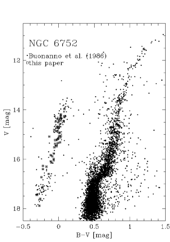
Figure 1: The colour-magnitude diagram of NGC 6752 (Buonanno et al. buca86 (1986)). Stars analysed in this paper (including 10 stars discussed by Moehler et al. 1997b ) are marked by open squares (some of which overlap due to almost identical photometric data).

2 Observations

We selected our targets from the photographic photometry of Buonanno et al. (buca86 (1986), see Table 1 and Fig. 1). For our observations we used the ESO 1.52m telescope with the Boller & Chivens spectrograph and CCD #39 (2048$\times$2048 pixels, (15 $\mu$m)² pixel size, read-out noise 5.4 e^-, conversion factor 1.2 e^-/count). We used grating # 33 (65 Åmm^-1) to cover a wavelength of 3300 Å – 5300 Å. Combined with a slit width of 2″ we thus achieved a spectral resolution of 2.6 Å. The spectra were obtained on July 22-25, 1998. For calibration purposes we observed each night ten bias frames and ten dome flat-fields with a mean exposure level of about 10,000 counts each. Before and after each science observation we took HeAr spectra for wavelength calibration purposes. We observed dark frames of 3600 and 1800 sec duration to measure the dark current of the CCD. As flux standard stars we used LTT 7987 and EG 274.

We also analyse data that were obtained as backup targets at the NTT during observing runs dedicated to other programs (60.E-0145, 61.E-0361). The observational set-up and the data reduction are described in Moehler et al. (mola99 (2000), 1999b ). These data have a much lower resolution of 5.4 Å.

3 Data Reduction

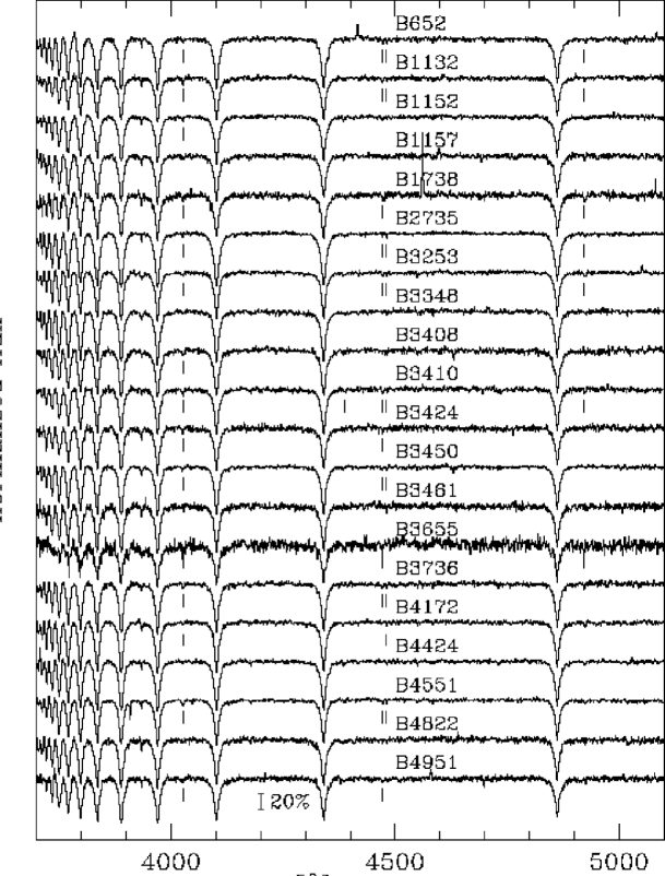
Figure 2: Normalized spectra of the programme stars that were observed at the ESO 1.52m telescope. The part shortward of 3900 Å was normalized by taking the highest flux point as continuum value. The He i lines $\lambda\lambda$ 4026 Å, 4388 Å, 4471 Å, 4922 Å, and the Mg ii line 4481 Å are marked (if visible in the spectrum).

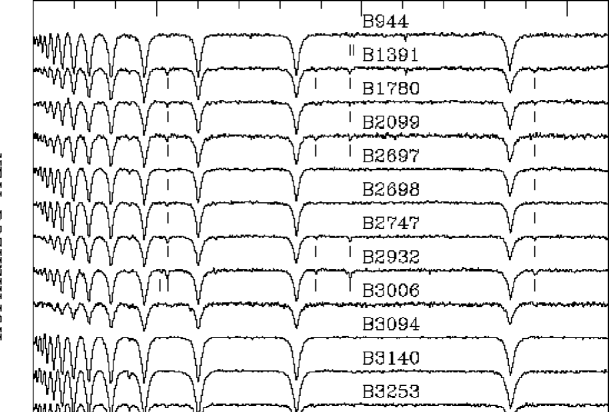
Figure 3: Normalized spectra of the programme stars that were observed at the NTT during 1997 and 1998. See Fig. 2 for details.

We first averaged the bias and flat field frames separately for each night. As we could not detect any significant change in the mean bias level we computed the median of the bias frames of the four nights and found that the bias level showed a gradient across the image, increasing from the lower left corner to the upper right corner by about 1%. We fitted the bias with a linear approximation along both axes and used this fit as a bias for the further reduction. As no overscan was recorded we could not adjust the bias level. Bias frames taken during the night, however, revealed no significant change in the mean bias level. The mean dark current determined from long dark frames showed no structure and turned out to be negligible (3$\pm$3 e^-/hr/pixel).

We determined the spectral energy distribution of the flat field lamp by averaging the mean flat fields of each night along the spatial axis. These one-dimensional “flat field spectra” were then heavily smoothed and used afterwards to normalize the dome flats along the dispersion axis. The normalized flat fields of the first three nights were combined. For the fourth night we used only the flat field obtained during that night as we detected a slight variation in the fringe patterns of the flat fields from the first three nights compared to that of the fourth (below 5%).

For the wavelength calibration we fitted 3^rd-order polynomials to the dispersion relations of the HeAr spectra which resulted in mean residuals of $\leq$0.1 Å. We rebinned the frames two-dimensionally to constant wavelength steps. Before the sky fit the frames were smoothed along the spatial axis to erase cosmic ray hits in the background. To determine the sky background we had to find regions without any stellar spectra, which were sometimes not close to the place of the object’s spectrum. Nevertheless the flat field correction and wavelength calibration turned out to be good enough that a linear fit to the spatial distribution of the sky light allowed the sky background at the object’s position to be reproduced with sufficient accuracy. This means in our case that after the fitted sky background was subtracted from the unsmoothed frame we do not see any absorption lines caused by the predominantly red stars of the clusters. The sky-subtracted spectra were extracted using Horne’s (horn86 (1986)) algorithm as implemented in MIDAS (Munich Image Data Analysis System).

Finally the spectra were corrected for atmospheric extinction using the extinction coefficients for La Silla (Tüg tueg77 (1977)) as implemented in MIDAS. The data for the flux standard stars were taken from Hamuy et al. (hamu92 (1992)) and the response curves were fitted by splines. The flux-calibration is helpful for the later normalization of the spectra as it takes out all large-scale sensitivity variations of the instrumental setup. Absolute photometric accuracy is not an issue here.

Table 2: Physical parameters, helium abundances, and masses for the target stars in NGC 6752 as derived using metal-poor model atmospheres. We used the photometry of Buonanno et al. (buca86 (1986)) to derive the masses.

Star	$T_{\rm eff}$	$\log\,g$	$\log{\frac{n_{\rm He}}{n_{\rm H}}}$	M
	[K]	[cm s-2]		[M⊙]
ESO 1.52m telescope observations in 1998
652	12500$\pm$310	3.86$\pm$0.09	$-$2.00$\pm$0.35	0.55
1132	17300$\pm$520	4.31$\pm$0.09	$-$2.46$\pm$0.16	0.50
1152	15700$\pm$360	4.19$\pm$0.05	$-$2.57$\pm$0.17	0.50
1157	15800$\pm$460	4.14$\pm$0.09	$-$2.89$\pm$0.31	0.50
1738	16700$\pm$700	4.15$\pm$0.12	$-$2.24$\pm$0.28	0.32
2735	11100$\pm$260	3.78$\pm$0.12	$-$1.14$\pm$0.36	0.73
3253	13700$\pm$390	3.80$\pm$0.09	$-$2.41$\pm$0.29	0.50
3348	12000$\pm$270	3.73$\pm$0.07	$-$2.18$\pm$0.38	0.65
3408	14600$\pm$400	4.21$\pm$0.09	$-$2.40$\pm$0.36	0.63
3410	15500$\pm$460	4.14$\pm$0.09	$-$2.22$\pm$0.19	0.41
3424	17900$\pm$570	4.23$\pm$0.09	$-$2.60$\pm$0.21	0.44
3450	13200$\pm$290	3.84$\pm$0.07	$-$2.05$\pm$0.24	0.43
3461	15200$\pm$500	4.18$\pm$0.09	$\leq-$3	0.70
3655	25800$\pm$1300	5.15$\pm$0.16	$-$2.32$\pm$0.24	0.68
3736	13400$\pm$370	3.91$\pm$0.09	$-$1.84$\pm$0.17	0.67
4172	12200$\pm$260	3.68$\pm$0.07	$-$2.24$\pm$0.54	0.46
4424	13000$\pm$290	3.99$\pm$0.07	$-$2.36$\pm$0.38	0.69
4551	15400$\pm$530	3.96$\pm$0.09	$-$2.21$\pm$0.24	0.39
4822	13900$\pm$450	3.91$\pm$0.09	$-$2.24$\pm$0.28	0.37
4951	17300$\pm$580	4.38$\pm$0.09	$-$2.63$\pm$0.22	0.56
ESO NTT observations in 1997
944	11100$\pm$230	3.70$\pm$0.10	$-$0.84$\pm$0.31	0.52
1391	19700$\pm$570	4.49$\pm$0.09	$-$2.04$\pm$0.10	0.39
1780	18000$\pm$580	4.40$\pm$0.09	$-$2.31$\pm$0.14	0.39
2099	20000$\pm$820	4.61$\pm$0.12	$-$2.38$\pm$0.22	0.48
ESO NTT observations in 1998
2697	15700$\pm$400	4.08$\pm$0.07	$-$2.36$\pm$0.17	0.91
2698	15400$\pm$610	4.11$\pm$0.10	$-$2.07$\pm$0.28	0.49
2747	22700$\pm$650	4.85$\pm$0.09	$-$2.16$\pm$0.10	0.61
2932	18600$\pm$700	4.63$\pm$0.12	$-$1.57$\pm$0.12	0.47
3006	30000$\pm$640	5.19$\pm$0.09	$\leq-$3	0.71
3094	10400$\pm$120	3.81$\pm$0.17	$-$1.83$\pm$1.35	1.09
31401	8000$\pm$100	2.84$\pm$0.14	$-$1.00$\pm$0.00	0.28
3253	13700$\pm$470	3.75$\pm$0.10	$-$1.85$\pm$0.31	0.45
3699	22900$\pm$990	4.64$\pm$0.12	$-$2.29$\pm$0.10	0.35
ESO NTT observations in 1993
491	29000$\pm$520	5.41$\pm$0.07	$\leq-$3	0.38
916	30200$\pm$430	5.61$\pm$0.07	$-$1.71$\pm$0.05	0.48
1509	17400$\pm$630	4.10$\pm$0.10	$-$2.17$\pm$0.16	0.26
1628	21800$\pm$590	4.83$\pm$0.09	$-$2.53$\pm$0.12	0.47
2162	33400$\pm$390	5.78$\pm$0.07	$-$1.94$\pm$0.09	0.45
2395	22200$\pm$690	5.10$\pm$0.09	$-$1.78$\pm$0.07	0.57
3915	31300$\pm$510	5.55$\pm$0.09	$\leq-$3	0.59
3975	21700$\pm$460	4.97$\pm$0.07	$-$2.04$\pm$0.10	0.67
4009	30700$\pm$920	5.61$\pm$0.12	$\leq-$3	0.54
4548	22000$\pm$1380	5.11$\pm$0.19	$-$2.02$\pm$0.16	0.67

1	This star is omitted from further analysis as it lies in
	a temperature range that is difficult to analyse and
	not of great interest for our discussion.

4 Atmospheric Parameters

To derive effective temperatures, surface gravities and helium abundances we fitted the observed Balmer and helium lines with stellar model atmospheres. Beforehand we corrected the spectra for radial velocity shifts, derived from the positions of the Balmer and helium lines. The resulting heliocentric velocities are listed in Table 1. The error of the velocities (as estimated from the scatter of the velocities derived from individual lines) is about 40 km s^-1. The spectra were then normalized by eye and are plotted in Figs. 2 and 3.

To establish the best fit we used the routines developed by Bergeron et al. (besa92 (1992)) and Saffer et al. (sabe94 (1994)), which employ a $\chi^{2}$ test. The $\sigma$ necessary for the calculation of $\chi^{2}$ is estimated from the noise in the continuum regions of the spectra. The fit program normalizes model spectra and observed spectra using the same points for the continuum definition.

We computed model atmospheres using ATLAS9 (Kurucz kuru91 (1991)) and used Lemke’s version of the LINFOR program (developed originally by Holweger, Steffen, and Steenbock at Kiel University) to compute a grid of theoretical spectra which include the Balmer lines H_α to H₂₂ and He i lines. The grid covered the range 7,000 K $\leq$ $T_{\rm eff}$ $\leq$ 35,000 K, 2.5 $\leq$ $\log\,g$ $\leq$ 6.0, $-3.0$ $\leq$ $\log{\frac{n_{\rm He}}{n_{\rm H}}}$ $\leq$ $-1.0$, at a metallicity of [M/H] = $-1.5$. In Table 2 we list the results obtained from fitting the Balmer lines H_β to H₁₀ (excluding H_ϵ to avoid the Ca ii H line) and the He i lines 4026 Å, 4388 Å, 4471 Å, and 4921 Å. The errors given are r.m.s. errors derived from the $\chi^{2}$ fit (see Moehler et al. 1999b for more details). These errors are obtained under the assumption that the only error source is statistical noise (derived from the continuum of the spectrum). However, errors in the normalization of the spectrum, imperfections of flat field/sky background correction, variations in the resolution (e.g. due to seeing variations when using a rather large slit width) and other effects may produce systematic rather than statistic errors, which are not well represented by the error obtained from the fit routine. Systematic errors can only be quantified by comparing truly independent analyses of the same stars. As this is not possible here we use our experience with the analysis of similar stars and estimate the true errors to be about 10% in $T_{\rm eff}$ and 0.15 dex in $\log\,g$ (cf. Moehler et al. 1997b , mola98 (1998)). Two stars show $B-V$ colours that are significantly redder than expected from their effective temperatures (B 2697: $B-V$ = $\rm+0\stackrel{{\scriptstyle m}}{{.}}08$, $T_{\rm eff}$ = 15,700 K; B 3006: $B-V$ = $\rm-0\stackrel{{\scriptstyle m}}{{.}}10$, $T_{\rm eff}$ = 30,000 K), possibly indicating that the colours are affected by binarity or photometric blending with a cool star. While the spectra look quite normal, we will not include these stars in any statistical discussion below. To increase our data sample we reanalysed the NTT spectra described and analysed by Moehler et al. (1997b ). We did not reanalyse the EFOSC1 data published in the same paper as they are of worse quality. We find that the atmospheric parameters determined by line profile fitting agree rather well with those published by Moehler et al. (1997b ).

The temperatures and gravities obtained from these metal-poor atmospheres are compared with the values predicted by canonical HB tracks in Fig. 4 (top panel). These tracks, which were computed for a main sequence mass of 0.805 M_⊙, an initial helium abundance Y of 0.23 and a scaled-solar metallicity [M/H] of $-$1.54, define the locus of canonical HB models which lose varying amounts of mass during the RGB phase. According to the Reimers mass-loss formulation the value of the mass-loss parameter $\eta_{R}$ would vary from $\approx$0.4 at the red end of the observed HB in NGC 6752 to $\approx$0.7 for the sdB stars, given the present composition parameters.

One can see from Fig. 4 (top panel) that the HBB stars in NGC 6752 show the same effect as seen in other globular clusters, namely, an offset from the zero-age horizontal branch (ZAHB) towards lower surface gravities over the temperature range 4.05 $<$ $\log\,T_{\rm eff}$ $<$ 4.30 (11,200 K $<$ $T_{\rm eff}$ $<$ 20,000 K). At lower or higher temperatures the gravities agree with the locus of the canonical HB tracks.

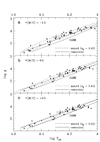
Figure 4: a-c. Temperatures and gravities of the programme stars in NGC 6752. a determined using model atmospheres with cluster metallicity ([M/H] = $-$1.5), b adopting a solar metallicity ([M/H] = 0) for the model atmospheres, c adopting a super-solar metallicity ([M/H] = $+$0.5) for the model atmospheres (see Sect. 4.1 for details). The dashed lines mark the locus of the HB evolutionary tracks for [M/H] = $-$1.54, as computed with helium mixing for the indicated values of the Reimers mass-loss parameter $\eta_{R}$ (see Sect. 4.2 for details). The solid lines mark the locus of canonical HB tracks for [M/H] = $-$1.54. These loci define the region within which the HB models spend 99 percent of their HB lifetime. Representative error bars are plotted.

4.1 Radiative levitation of heavy elements

As described in Moehler et al. (1999a , see also Fig. 5), we found evidence for iron enrichment in the spectra of the HBB stars obtained at the ESO 1.52m telescope, whereas the magnesium abundance appeared consistent with the cluster magnesium abundance. The actual iron abundances derived for these stars by fitting the iron lines in the ESO 1.52m spectra are listed in Table 4. The mean iron abundance turns out to be [Fe/H] = $+0.12\pm 0.40$ (internal errors only, $\log\epsilon_{Fe}=7.58$) for stars hotter than about 11,500 K – in good agreement with the findings of Behr et al. (beco99 (1999), 2000b ) for HBB/HBA (horizontal branch A type) stars in M 13 and M 15 and Glaspey et al. (glmi89 (1989)) for two HBB/HBA stars in NGC 6752. This iron abundance is a factor of 50 greater than that of the cluster, but still a factor of 3 smaller than that required to explain the Strömgren $u$-jump discussed by Grundahl et al. (grca99 (1999), $\log\epsilon_{Fe}=8.1$). The mean magnesium abundance for the same stars is [Mg/H] = $-1.13\pm 0.29$ (internal errors only), corresponding to [Mg/Fe] = $+$0.4 for [Fe/H] = $-$1.54. This value agrees well with the abundance [Mg/Fe] = $+0.4$ found by Norris & da Costa (1995b ) for red giants in NGC 6752.

The abundances are plotted versus temperature in Fig. 5. The trend of decreasing helium abundance with increasing temperature seen in the ESO 1.52m data (and also reported by Behr et al. beco99 (1999) for HB stars in M 13) is not supported towards higher temperatures by the NTT data. This could be due to the lower resolution of the NTT data which may tend to overestimate abundances (Glaspey et al. glmi89 (1989)).

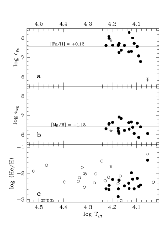
Figure 5: a-c Abundances of iron (a), magnesium (b), and helium (c) for the programme stars in NGC 6752. The filled symbols mark stars which have been observed at higher resolution at the ESO 1.52m telescope, the open symbols mark stars observed at the NTT. Only the helium abundance could be derived for the NTT stars due to the low resolution of the data. The asterisk marks the results of Glaspey et al. (glmi89 (1989)) for an HBB star in NGC 6752. Upper limits are marked by arrows.

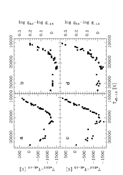
Figure 6: a-d This plot shows the differences in effective temperature (a,c) and surface gravity (b,d) derived from fits with model atmospheres of different metallicity (solar$-$metal-poor [a,b], metal-rich$-$metal-poor [c,d]). It is obvious that an increase in the metallicity of the model atmospheres usually decreases the resulting temperatures and increases the resulting surface gravities.

As iron is very important for the temperature stratification of stellar atmospheres we tried to take the increased iron abundance into account by computing model atmospheres for [M/H] = 0. Indeed a backwarming effect of 2–4% on the temperature structure was found in the formation region of the Balmer lines, when comparing solar composition models with the metal-poor models. We then repeated the fit to derive $T_{\rm eff}$, $\log\,g$, and $\log{\frac{n_{\rm He}}{n_{\rm H}}}$ with these enriched model atmospheres. The resulting effective temperatures and gravities changed as displayed in Fig. 6. The results are listed in Table 3 and plotted in Fig. 4 (central panel). From Fig. 4 (central panel) it is clear that the use of solar-metallicity model atmospheres moves most stars closer to the canonical zero-age horizontal branch (ZAHB) due to a combination of lower $T_{\rm eff}$ and/or higher $\log\,g$. The three stars between 10,000 K and 12,000 K, however, fall below the canonical ZAHB when fitted with enriched model atmospheres. This is plausible as the radiative levitation is supposed to start around 11,000 – 12,000 K (Grundahl et al. grca99 (1999)) and the cooler stars therefore should have metal-poor atmospheres (see also Fig. 5, where the coolest analysed star shows no evidence of iron enrichment). This assumption is also supported by the results of Glaspey et al. (glde85 (1985), NGC 6397; glmi89 (1989), NGC 6752) and Behr et al. (beco99 (1999), M 13; 2000b , M 15). Now the stars below 15,300 K scatter around the locus defined by the canonical HB tracks. The stars between 15,500 K and 19,000 K, however, still show offsets from the canonical locus while for the sdB stars not much is changed. Interestingly, 15,500 K is roughly the temperature at which the stars in NGC 6752 return to the ZAHB in ($u-y$, $u$) of Grundahl et al. (grca99 (1999)). Grundahl et al. caution, however, that their faint photometry for NGC 6752 might be affected by poor seeing, and that in the Strömgren CMD of the better observed cluster, M13, the stars do not return to the ZAHB until a temperature of about 20,000 K.

Table 3: Physical parameters, helium abundances, and masses for the target stars in NGC 6752 as derived using solar metallicity model atmospheres.

Star	$T_{\rm eff}$	$\log\,g$	$\log{\frac{n_{\rm He}}{n_{\rm H}}}$	M
	[K]	[cm s-2]		[M⊙]
ESO 1.52m telescope observations in 1998
652	12500$\pm$230	3.98$\pm$0.07	$-$2.19$\pm$0.36	0.67
1132	16300$\pm$460	4.31$\pm$0.07	$-$2.45$\pm$0.16	0.51
1152	15000$\pm$290	4.21$\pm$0.05	$-$2.58$\pm$0.17	0.52
1157	15000$\pm$360	4.15$\pm$0.07	$-$2.89$\pm$0.31	0.52
1738	15800$\pm$580	4.15$\pm$0.10	$-$2.23$\pm$0.28	0.32
2735	11400$\pm$170	3.96$\pm$0.07	$-$1.51$\pm$0.28	0.98
3253	13500$\pm$310	3.88$\pm$0.07	$-$2.57$\pm$0.28	0.57
3348	12100$\pm$220	3.86$\pm$0.07	$-$2.44$\pm$0.38	0.80
3408	14100$\pm$330	4.24$\pm$0.07	$-$2.47$\pm$0.36	0.66
3410	14900$\pm$370	4.17$\pm$0.07	$-$2.25$\pm$0.19	0.43
3424	16800$\pm$510	4.21$\pm$0.09	$-$2.58$\pm$0.22	0.43
3450	13000$\pm$210	3.92$\pm$0.05	$-$2.22$\pm$0.24	0.49
3461	14600$\pm$400	4.20$\pm$0.09	$\leq-$3	0.73
3655	24900$\pm$1250	5.14$\pm$0.16	$-$2.32$\pm$0.24	0.65
3736	13200$\pm$270	3.99$\pm$0.07	$-$1.98$\pm$0.17	0.77
4172	12300$\pm$200	3.81$\pm$0.05	$-$2.49$\pm$0.55	0.57
4424	12900$\pm$210	4.07$\pm$0.05	$-$2.58$\pm$0.40	0.78
4551	14900$\pm$410	3.99$\pm$0.09	$-$2.26$\pm$0.24	0.41
4822	13600$\pm$350	3.97$\pm$0.09	$-$2.37$\pm$0.28	0.41
4951	16300$\pm$520	4.38$\pm$0.09	$-$2.61$\pm$0.22	0.57
ESO NTT observations in 1997
944	11400$\pm$190	3.90$\pm$0.09	$-$1.27$\pm$0.22	0.74
1391	18500$\pm$570	4.45$\pm$0.09	$-$2.02$\pm$0.10	0.36
1780	16900$\pm$530	4.37$\pm$0.09	$-$2.28$\pm$0.14	0.37
2099	18800$\pm$790	4.58$\pm$0.10	$-$2.36$\pm$0.22	0.46
ESO NTT observations in 1998
2697	15000$\pm$360	4.10$\pm$0.07	$-$2.39$\pm$0.17	0.94
2698	14700$\pm$490	4.13$\pm$0.10	$-$2.10$\pm$0.26	0.50
2747	21600$\pm$700	4.80$\pm$0.09	$-$2.16$\pm$0.10	0.55
2932	17500$\pm$600	4.61$\pm$0.10	$-$1.54$\pm$0.10	0.46
3006	29100$\pm$740	5.18$\pm$0.09	$\leq-$3	0.68
3094	10800$\pm$310	4.01$\pm$0.14	$-$2.33$\pm$1.97	1.52
3253	13300$\pm$370	3.81$\pm$0.09	$-$1.95$\pm$0.31	0.50
3699	21800$\pm$1050	4.60$\pm$0.12	$-$2.30$\pm$0.10	0.32
ESO NTT observations in 1993
491	28100$\pm$540	5.40$\pm$0.07	$\leq-$3	0.37
916	29400$\pm$480	5.60$\pm$0.07	$-$1.70$\pm$0.05	0.46
1509	16400$\pm$510	4.07$\pm$0.09	$-$2.15$\pm$0.16	0.24
1628	20600$\pm$620	4.78$\pm$0.09	$-$2.52$\pm$0.12	0.43
2162	33400$\pm$460	5.79$\pm$0.07	$-$1.92$\pm$0.09	0.44
2395	21000$\pm$750	5.06$\pm$0.10	$-$1.78$\pm$0.09	0.53
3915	30700$\pm$620	5.54$\pm$0.09	$\leq-$3	0.56
3975	20400$\pm$520	4.92$\pm$0.07	$-$2.02$\pm$0.12	0.62
4009	30100$\pm$1120	5.60$\pm$0.14	$\leq-$3	0.52
4548	20700$\pm$1490	5.06$\pm$0.19	$-$2.00$\pm$0.17	0.62

Table 4: Helium, iron, and magnesium abundances of the HBB stars observed with the ESO 1.52m telescope (except B 3655, which has a too noisy spectrum). [Fe/H] and [Mg/H] are derived using solar abundances of $\log\epsilon_{\rm Fe,\odot}=7.46$ and $\log\epsilon_{\rm Mg,\odot}=7.53$. The physical parameters and the helium abundances are taken from Table 3.

Star	$T_{\rm eff}$	$\log\,g$	$\log{\frac{n_{\rm He}}{n_{\rm H}}}$	[Fe/H]	[Mg/H]
	[K]	[cm s-2]
652	12500	3.98	$-$2.19	$+$0.1	$-$0.9
1132	16300	4.31	$-$2.45	$+$0.5	$-$1.0
1152	15000	4.21	$-$2.58	$+$0.2	$-$1.4
1157	15000	4.15	$-$2.89	$+$0.2	$-$1.2
1738	15800	4.15	$-$2.23	$+$0.2	$-$0.9
2735	11400	3.96	$-$1.51	$<-$1.6	$-$1.5
3253	13500	3.88	$-$2.57	$+$0.8	$-$1.3
3348	12100	3.86	$-$2.44	$-$0.2	$-$1.1
3408	14100	4.24	$-$2.47	$+$0.2	$-$1.3
3410	14900	4.17	$-$2.25	$+$0.6	$-$1.5
3424	16800	4.21	$-$2.58	$-$0.1	$-$1.2
3450	13000	3.92	$-$2.22	$-$0.4	$-$1.2
3461	14600	4.20	$\leq-$3	$+$0.3	$-$0.7
3736	13200	3.99	$-$1.98	$+$0.3	$-$0.9
4172	12300	3.81	$-$2.49	$-$0.2	$-$1.7
4424	12900	4.07	$-$2.58	$+$0.6	$-$1.5
4551	14900	3.99	$-$2.26	$-$0.9	$-$0.6
4822	13600	3.97	$-$2.37	$-$0.2	$-$0.9
4951	16300	4.38	$-$2.61	$+$0.2	$-$1.0

We next repeated the Balmer line profile fits by increasing the metal abundance of the model atmospheres to [M/H]=$+$0.5 (see Fig. 4, bottom panel, and Table 5), which did not significantly change the resulting values for $T_{\rm eff}$ and $\log\,g$. In particular, note that especially the “deviant” stars (now between 15,300 K and 19,000 K) remain offset from the canonical ZAHB.

Table 5: Physical parameters, helium abundances, and masses for the target stars in NGC 6752 as derived using metal-rich model atmospheres.

Star	$T_{\rm eff}$	$\log\,g$	$\log{\frac{n_{\rm He}}{n_{\rm H}}}$	M
	[K]	[cm s-2]		[M⊙]
ESO 1.52m telescope observations in 1998
652	12700$\pm$220	4.05$\pm$0.07	$-$2.40$\pm$0.36	0.73
1132	16300$\pm$430	4.36$\pm$0.07	$-$2.55$\pm$0.14	0.54
1152	15100$\pm$290	4.26$\pm$0.05	$-$2.71$\pm$0.16	0.55
1157	15100$\pm$370	4.20$\pm$0.07	$-$2.98$\pm$0.26	0.55
1738	15900$\pm$540	4.21$\pm$0.10	$-$2.37$\pm$0.26	0.35
2735	11600$\pm$180	4.08$\pm$0.07	$-$1.74$\pm$0.24	1.20
3253	13700$\pm$300	3.94$\pm$0.07	$-$2.76$\pm$0.24	0.61
3348	12300$\pm$210	3.94$\pm$0.07	$-$2.65$\pm$0.36	0.89
3408	14200$\pm$310	4.30$\pm$0.07	$-$2.64$\pm$0.35	0.71
3410	15000$\pm$350	4.23$\pm$0.07	$-$2.40$\pm$0.19	0.47
3424	16700$\pm$490	4.24$\pm$0.09	$-$2.66$\pm$0.21	0.43
3450	13200$\pm$200	3.99$\pm$0.05	$-$2.45$\pm$0.26	0.53
3461	14700$\pm$380	4.26$\pm$0.09	$-$3.37$\pm$0.33	0.79
3655	25000$\pm$170	5.16$\pm$0.16	$-$2.31$\pm$0.24	0.64
3736	13400$\pm$260	4.07$\pm$0.07	$-$2.17$\pm$0.17	0.86
4172	12500$\pm$200	3.88$\pm$0.05	$-$2.70$\pm$0.50	0.62
4424	13000$\pm$210	4.13$\pm$0.05	$-$2.79$\pm$0.35	0.84
4551	15000$\pm$400	4.05$\pm$0.09	$-$2.43$\pm$0.24	0.44
4822	13800$\pm$340	4.04$\pm$0.09	$-$2.59$\pm$0.28	0.44
4951	16300$\pm$480	4.42$\pm$0.09	$-$2.72$\pm$0.21	0.60
ESO NTT observations in 1997
944	11600$\pm$180	4.00$\pm$0.07	$-$1.52$\pm$0.19	0.87
1391	18400$\pm$580	4.48$\pm$0.09	$-$2.08$\pm$0.10	0.37
1780	16900$\pm$500	4.41$\pm$0.09	$-$2.37$\pm$0.12	0.39
2099	18700$\pm$810	4.60$\pm$0.10	$-$2.41$\pm$0.22	0.46
ESO NTT observations in 1998
2697	15000$\pm$330	4.14$\pm$0.07	$-$2.52$\pm$0.17	0.98
2698	14800$\pm$490	4.20$\pm$0.10	$-$2.25$\pm$0.28	0.55
2747	21500$\pm$830	4.81$\pm$0.09	$-$2.17$\pm$0.10	0.54
2932	17300$\pm$570	4.65$\pm$0.10	$-$1.61$\pm$0.10	0.49
3006	29300$\pm$590	5.19$\pm$0.07	$-$3.01$\pm$0.31	0.65
3094	11100$\pm$290	4.14$\pm$0.10	$-$2.54$\pm$1.97	1.87
3253	13500$\pm$350	3.87$\pm$0.09	$-$2.12$\pm$0.31	0.54
3699	21800$\pm$030	4.61$\pm$0.12	$-$2.31$\pm$0.10	0.31
ESO NTT observations in 1993
491	28000$\pm$520	5.40$\pm$0.07	$-$3.40$\pm$0.14	0.35
916	29300$\pm$460	5.59$\pm$0.05	$-$1.70$\pm$0.05	0.43
1509	16400$\pm$500	4.11$\pm$0.09	$-$2.25$\pm$0.16	0.26
1628	20700$\pm$720	4.81$\pm$0.09	$-$2.55$\pm$0.12	0.43
2162	33400$\pm$500	5.78$\pm$0.07	$-$1.91$\pm$0.09	0.41
2395	20900$\pm$810	5.07$\pm$0.09	$-$1.80$\pm$0.09	0.52
3915	30600$\pm$580	5.54$\pm$0.07	$-$3.19$\pm$0.19	0.53
3975	20300$\pm$580	4.94$\pm$0.07	$-$2.06$\pm$0.12	0.62
4009	30100$\pm$040	5.62$\pm$0.12	$-$3.14$\pm$0.19	0.51
4548	20400$\pm$590	5.06$\pm$0.19	$-$2.03$\pm$0.17	0.60

4.2 Helium mixing

As outlined in Sect. 1, helium mixing during the RGB phase may also be able to explain the low gravities of the HBB stars. Under this scenario the mixing currents within the radiative zone below the base of the convective envelope of a red giant star are assumed to penetrate into the top of the hydrogen shell where helium is being produced by the hydrogen burning reactions. Ordinarily one would expect the gradient in the mean molecular weight $\mu$ to prevent any penetration of the mixing currents into the shell. If, however, the timescale for mixing were shorter than the timescale for nuclear burning, then the helium being produced at the top of the shell might be mixed outward into the envelope before a $\mu$ gradient is established. Under these circumstances a $\mu$ gradient would not inhibit deep mixing simply because such a gradient would not exist within the mixed region.

Since deep mixing is presumably driven by rotation, one would expect a more rapidly rotating red giant to show a larger increase in the envelope helium abundance. This, in turn, would lead to a brighter RGB tip luminosity and hence to greater mass loss. The progeny of the more rapidly rotating giants should therefore lie at higher effective temperatures along the HB than the progeny of the more slowly rotating giants. This predicted increase in the stellar rotational velocity with effective temperature along the HB has not, however, been confirmed by the recent observations of M13 by Behr et al. (2000a ). These observations show that HB stars in M13 hotter than 11,000 K are, in fact, rotating slowly with $v\sin i<$ 10 km s^-1 in contrast to the cooler HB stars where rotational velocities as high as 40 km s^-1 are found (see also Peterson et al. pero95 (1995)).

There are a couple of possible explanations for this apparent discrepancy. One possibility is that the greater mass loss suffered by the HBB stars might carry away so much angular momentum that the surface layers are spun down even though the core is still rotating rapidly. Alternatively Sills & Pinsonneault (sipi00 (2000)) have suggested that the observed gravitational settling of helium in HBB stars might set up a $\mu$ gradient in the outer layers which inhibits the transfer of angular momentum from the rapidly rotating interior to the surface. Thus the surface rotational velocities may not necessarily be indicative of the interior rotation.

In order to explore the consequences of helium mixing for the HBB stars quantitatively, we evolved a set of 13 sequences up the RGB to the helium flash for varying amounts of helium mixing using the approach of Sweigart (1997a , 1997b ). As in the case of the canonical models discussed previously, all of these mixed sequences had an initial helium abundance Y of 0.23 and a scaled-solar metallicity [M/H] of $-$1.54. The main-sequence mass was taken to be 0.805 M_⊙, corresponding to an age at the tip of the RGB of 15 Gyr. The mixing depth, as defined by the parameter $\Delta X_{mix}$ of Sweigart (1997a , 1997b ), ranged from 0.0 (canonical, unmixed case) to 0.24 in increments of 0.02. Mass loss via the Reimers formulation was included in the calculations with the mass-loss parameter $\eta_{R}$ set equal to 0.40. This value for $\eta_{R}$ was chosen so that a canonical, unmixed model would lie near the red end of the observed blue HB in NGC 6752. Both the mixing and mass loss were turned off once the models reached the core He flash at the tip of the RGB, and the subsequent evolution was then followed through the helium flash to the end of the HB phase using standard techniques.

We did not investigate the changes in the surface abundances of CNO, Na and Al caused by the helium mixing, since such a study was beyond the scope of the present paper. Rather, our objective was to determine how the mixing affected those quantities which impact on the HB evolution, i.e., envelope helium abundance and mass. We do note that the mixing in the more deeply mixed RGB models would have penetrated into regions of substantial Na and Al production according to the calculations of Cavallo et al. (casw96 (1996), casw98 (1998)). However, the resulting changes in the surface Na and Al abundances will depend on the assumed initial Ne and Mg isotopic abundances and on the adopted nuclear reaction rates, which in some cases are quite uncertain.

The locus of the above helium-mixed sequences in the $\log\,g$ - $\log\,T_{\rm eff}$ plane is indicated by the dashed lines in the top panel of Fig. 4. The red end of the mixed ZAHB in this panel, located at $\log\,T_{\rm eff}$  = 3.93, is set by the canonical, unmixed sequence for the present set of model parameters. Since mixing increases the RGB mass loss, a mixed HB model will have a higher effective temperature than the corresponding canonical model. At the same time mixing increases the envelope helium abundance in the HB model, which, in turn, increases both the hydrogen-burning and surface luminosities. The net effect is to shift the mixed locus in Fig. 4 towards lower gravities with increasing $T_{\rm eff}$ compared to the canonical locus, until a maximum offset is reached for 15,500 K $<$ $T_{\rm eff}$ $<$ 19,000 K. At higher temperatures the mixed locus shifts back towards the canonical locus, as the contribution of the hydrogen shell to the surface luminosity declines due to the decreasing envelope mass. The predicted locus along the extreme HB (EHB) does not depend strongly on the extent of the mixing, since the luminosities and gravities of the EHB stars are primarily determined by the mass of the helium core, which is nearly the same for the mixed and canonical models. Overall the variation of $\log\,g$ with $T_{\rm eff}$ along the mixed locus in the top panel of Fig. 4 mimics the observed variation.

The results presented in Sect. 4.1 demonstrate that radiative levitation of heavy elements can account for a considerable fraction of the gravity offset along the HBB, especially for temperatures cooler than 15,100 K. Consequently the amount of helium mixing required to explain the remaining offset between 15,300 K and 19,000 K is much less than the amount required to explain the offsets found without accounting for radiative levitation (top panel of Fig. 4). In order to compare the gravities predicted by the helium-mixing scenario with those derived from the metal-enhanced atmospheres, we computed a second set of mixed sequences using the same approach as above but with a larger value of the mass-loss parameter $\eta_{R}$, i.e., $\eta_{R}$ = 0.45. The red end of the mixed ZAHB for these sequences is located at $\log\,T_{\rm eff}$ = 4.01 and is therefore hotter than the red end of the mixed ZAHB for the sequences with $\eta_{R}$ = 0.40. The HB stars cooler than this temperature in NGC 6752 would then be identified with unmixed stars which lost less mass along the RGB.

By increasing the mass loss efficiency we reduce the amount of mixing needed to populate the temperature range 15,300 K $<$ $T_{\rm eff}$ $<$ 19,000 K and therefore the size of the resulting gravity offset. The locus of the mixed sequences with $\eta_{R}$ = 0.45 is indicated by the dashed lines in the central panel of Fig. 4. The gravity offsets along this mixed locus seem to provide a reasonable fit to the gravities given by the model atmospheres with solar metallicity.

Finally we computed a third set of mixed sequences with the mass-loss parameter increased further to $\eta_{R}$ = 0.50 for comparison with the gravities obtained from the atmospheres with super-solar metallicity in the bottom panel of Fig. 4. As expected, these mixed sequences show a smaller gravity offset in the temperature range 15,500 K $<$ $T_{\rm eff}$ $<$ 19,000 K. Moreover, the red end of the mixed ZAHB shifts blueward to $\log\,T_{\rm eff}$ = 4.08.

5 Masses

We calculated masses for the programme stars in NGC 6752 from their values of $T_{\rm eff}$ and $\log\,g$ using the equation:

$\log{\frac{\rm M}{\rm M_{\odot}}}=const.+\log g+0.4\cdot((m-M)_{V}-V+V_{th})$

where $V_{th}$ denotes the theoretical brightness at the stellar surface as given by Kurucz (kuru92 (1992)). We decided to use the photometry of Buonanno et al. (buca86 (1986)) to derive masses. As can be seen from Table 1 the photometry of Thompson et al. (thka99 (1999)) yields in general fainter visual magnitudes than the photometry of Buonanno et al. The effect on the masses, however, is small: On average, the masses derived from the Thompson et al. photometry are 5% lower than those derived from the Buonanno et al. photometry. We adopted $(m-M)_{0}=13.17$ and $E_{B-V}$ = 0.04 for the distance modulus and reddening. These are mean values derived from the determinations of Renzini et al. (rebr96 (1996)), Reid (reid97 (1997), reid98 (1998)), and Gratton et al. (grfu97 (1997)). The errors in $\log{\rm M}$ are estimated to be about the same as obtained for the older NGC 6752 data described by Moehler et al. (1997b ): 0.15 dex for stars above the gap, 0.17 dex for stars within the gap region and 0.22 dex for stars below the gap.

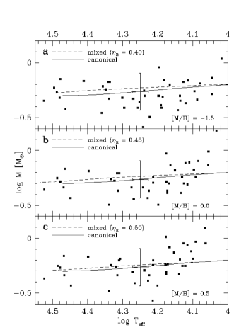
Figure 7: a-c Temperatures and masses (derived from Buonanno et al.’s photometry) of the programme stars in NGC 6752. a determined using model atmospheres with cluster metallicity ([M/H] = $-$1.5), b adopting a solar metallicity ([M/H] = 0) for the model atmospheres c adopting a super–solar metallicity ([M/H] = $+$0.5) for the model atmospheres. For more details see Sect. 4.1. The dashed resp. solid lines mark the ZAHB masses for a metallicity [M/H] = $-$1.54, as computed with and without mixing, respectively. (see Sect. 4.2 and Fig. 4 for details).

Table 6: Mean mass ratios between spectroscopically derived masses and predicted zero-age HB masses at the same effective temperatures. B 2697, B 3006 and stars cooler than 11,500 K are excluded from this comparison. $\eta_{\rm R}$ gives the Reimers’ mass loss parameter for the respective ZAHB. We derived the masses using the photometry of Buonanno et al. (buca86 (1986)). The cited errors are standard deviations.

cool HBB stars	hot HBB stars	sdB stars	[M/H]	track
$0.89^{+0.20}_{-0.16}$ (16)	$0.76^{+0.21}_{-0.17}$ (9)	$1.04^{+0.25}_{-0.20}$ (12)	$-$1.5	canonical HB, variable $\eta_{\rm R}$
$0.84^{+0.19}_{-0.16}$ (16)	$0.70^{+0.19}_{-0.15}$ (9)	$0.95^{+0.23}_{-0.18}$ (12)	$-$1.5	mixed HB, $\eta_{\rm R}$ = 0.40
$0.97^{+0.24}_{-0.19}$ (16)	$0.73^{+0.22}_{-0.17}$ (9)	$0.97^{+0.23}_{-0.19}$ (12)	$+$0.0	canonical HB, variable $\eta_{\rm R}$
$0.94^{+0.23}_{-0.19}$ (16)	$0.69^{+0.20}_{-0.16}$ (9)	$0.91^{+0.22}_{-0.18}$ (12)	$+$0.0	mixed HB, $\eta_{\rm R}$ = 0.45
$1.06^{+0.27}_{-0.21}$ (16)	$0.76^{+0.22}_{-0.17}$ (9)	$0.95^{+0.24}_{-0.19}$ (12)	$+$0.5	canonical HB, variable $\eta_{\rm R}$
$1.04^{+0.27}_{-0.21}$ (16)	$0.73^{+0.21}_{-0.16}$ (9)	$0.90^{+0.22}_{-0.18}$ (12)	$+$0.5	mixed HB, $\eta_{\rm R}$ = 0.50

The masses derived from the analysis using metal-poor model atmospheres are plotted in Fig. 7 (top panel). The sdB stars hotter than 20,000 K ($\log\,T_{\rm eff}$ = 4.3) scatter around the canonical ZAHB, whereas the stars below 16,000 K ($\log\,T_{\rm eff}$ = 4.2) lie mainly below the canonical ZAHB. Even stronger deviations towards low masses are found between 16,000 K and 20,000 K. Comparing the masses to those predicted by the mixed ZAHB ($\eta_{\rm R}=$ 0.40) we obtain similar results. To quantify the offsets we compare the masses of the stars to those they would have on the theoretical ZAHB at the same $T_{\rm eff}$ (see Table 6). We divide the stars into three groups for the further discussion (excluding stars below 11,500 K, for which diffusion should play no rôle, as well as B 2697 and B 3006): cool HBB stars ($T_{\rm eff}$ $<$ 16,000 K, 16 stars), hot HBB stars (16,000 K $\leq$ $T_{\rm eff}$ $<$ 20,000 K, 9 stars), and sdB stars ($T_{\rm eff}$ $\geq$ 20,000 K, 12 stars). The effective temperatures here are those derived from metal-poor model atmospheres.

The results of the analyses using solar-metallicity model atmospheres are plotted in the central panel of Fig. 7 (see Table 6). The effect on the masses is similar to that on the temperatures/gravities (Fig. 4, central panel) – below 15,300 K (cool HBB stars) and above 20,000 K (sdB stars) the masses basically scatter around the canonical ZAHB, but the hot HBB stars between these two groups still show too low masses. Comparing the masses to those predicted by the mixed ZAHB ($\eta_{\rm R}$ = 0.45) gives similar results. As the stars become cooler when analysed with more metal-rich atmospheres the temperature boundaries were shifted to include the same stars as for the comparison made above.

Even the use of metal-rich model atmospheres for the analyses does not change much (see Table 6 and the bottom panel of Fig. 7). Obviously the hot HBB stars in the intermediate temperature range still show low masses, despite the use of metal-rich model atmospheres. Thus the problem of the stars in this temperature range(15,300 K$<$ $T_{\rm eff}$ $<$19,000 K) cannot be completely solved by the scaled-solar metal-rich atmospheres used here.

6 Discussion

We find that the atmospheres of HBB stars in NGC 6752 with $T_{\rm eff}$ $>$ 11,500 K are enriched in iron ([Fe/H] $\approx+$0.1) whereas their magnesium abundances are the same as found in cluster giants. Our results are consistent with those of Behr et al. (beco99 (1999), 2000b ) for HBB stars in M 13 and M 15. Using model atmospheres that try to take into account this enrichment in iron (and presumably other heavy elements) reconciles the atmospheric parameters of stars with 11,500 K $\leq$ $T_{\rm eff}$ $<$ 15,100 K with canonical expectations as suggested by Grundahl et al. (grca99 (1999)). Also the masses derived from these analyses are in good agreement with canonical predictions within this temperature range. However, we found that even with model atmospheres as metal rich as [M/H] = $+$0.5 the atmospheric parameters of the hot HBB stars (15,300 K $<$ $T_{\rm eff}$ $<$ 19,000 K) in NGC 6752 cannot be reconciled with the canonical ZAHB. Both the gravities and masses of these hot HBB stars remain too low. In addition, the masses for the stars below 15,100 K are slightly too high for the super-solar metallicity (the EHB stars are hardly affected at all by changes in the metallicity of the model atmospheres).

Michaud et al. (miva83 (1983)) noted that diffusion will not necessarily enhance all heavy elements by the same amount and that the effects of diffusion vary with effective temperature. Elements that were originally very rare may be enhanced even more strongly than iron (see also Behr et al. beco99 (1999), where P and Cr are enhanced to [M/H] $\geq+1$). The question of whether diffusion is the (one and only) solution to the “low gravity” problem cannot be answered without detailed abundance analyses to determine the actual abundances and the use of model atmospheres that allow the use of non-scaled solar abundances (like ATLAS12). We can, however, state that those model atmospheres, which reproduce the $u$-jump discussed by Grundahl et al. (grca99 (1999)) cannot completely reconcile the atmospheric parameters of hot HB stars with canonical theory. Model atmospheres with abundance distributions that may solve the discrepancy between theoretically predicted and observed atmospheric parameters of hot HB stars may then, in turn, not reproduce the Strömgren $u$-jump. It is intriguing that the temperature, at which the stars in $u,u-y$ seem to return to the ZAHB, is roughly the same at which they start to deviate again from the canonical ZAHB in $\log\,g$, $T_{\rm eff}$ when analysed with metal-rich atmospheres.

The stars between 15,300 K and 19,000 K (when analysed with metal-rich atmospheres) are currently best fit by a moderately mixed ZAHB. However, the fact that their masses are too low cautions against identifying He mixing as the only cause for these low gravities - because in this case the luminosities of the stars would be increased and canonical masses would result.

- (1) Behr B.B., Cohen J.G., McCarthy J.K., Djorgovski S.G., 1999, ApJ 517, L135
- (2) Behr B.B., Djorgovski S.G., Cohen J.G., McCarthy J.K., Côlé P., Piotto G., Zoccali M., 2000a, ApJ 528, 849
- (3) Behr B.B., Cohen J.G., McCarthy J.K., 2000b, ApJ 531, L37
- (4) Buonanno R., Caloi V., Castellani V., et al., 1986, A&AS 66, 79
- (5) Bergeron P., Saffer R.A., Liebert J., 1992, ApJ 394, 228
- (6) Caloi, V., 1999, A&A 343, 904
- (7) Carretta E., Gratton R., Sneden C., Bragaglia A., 2000, A&A 354, 169
- (8) Cavallo R.M., Sweigart A.V., Bell R.A., 1996, ApJ 464, L79
- (9) Cavallo R.M., Sweigart A.V., Bell R.A., 1998, ApJ 492, 575
- (10) Charbonnel C., 1995, ApJ 453, L41
- (11) Fujimoto M.Y., Aikawa M., Kato K., 1999, ApJ 519, 733
- (12) Glaspey J.W., Demers S., Moffat A.F.J., Shara M., 1985, ApJ 289, 326
- (13) Glaspey J.W., Michaud G., Moffat A.F.J., Demers S., 1989, ApJ 339, 926
- (14) Gratton R.G., Fusi Pecci F., Carretta E., et al., 1997, ApJ 491, 749
- (15) Grundahl F., Catelan M., Landsman W.B., Stetson P.B., Andersen M., 1999, ApJ 524, 242
- (16) Hamuy M., Walker A.R., Suntzeff N.B., et al., 1992, PASP 104, 533
- (17) Hanson R.B., Sneden C., Kraft R.P., Fulbright J., 1998, AJ 116, 1286
- (18) Heber U., Moehler S., Reid I.N., 1997, Masses and gravities of blue horizontal branch (BHB) stars revisited, In: Battrick B. (ed) HIPPARCOS Venice ’97, ESA SP-402, p. 461
- (19) Horne K., 1986, PASP 98, 609
- (20) Kraft R.P., 1994, PASP 106, 553
- (21) Kraft R.P., Sneden C., Smith G.H., et al., 1997, AJ 113,279
- (22) Kurucz R.L., 1991, private communication
- (23) Kurucz R.L., 1992, in The Stellar Populations of Galaxies, eds. B. Barbuy & A. Renzini, IAU Symp. 149 (Kluwer:Dordrecht), 225
- (24) Langer G.E., Hoffman R.D., 1995, PASP 107, 1177
- (25) Leone F., Manfrè M., 1997, A&A 320, 257
- (26) Michaud G., Vauclair G., Vauclair S., 1983, ApJ 267, 256
- (27) Mitchell K.J., Saffer R.A., Howell S.B., Brown T.M., 1998, MNRAS 295, 225
- (28) Moehler S., 1999, RvMA 12, p. 281
- (29) Moehler S., Heber U., Durrell P., 1997a, A&A 317, L83
- (30) Moehler S., Heber U., Rupprecht G., 1997b, A&A 319, 109
- (31) Moehler S., Landsman W., Napiwotzki R., 1998, A&A 335, 510
- (32) Moehler S., Sweigart A.V., Landsman W.B., Heber U., Catelan M., 1999a, A&A 346, L1
- (33) Moehler S., Sweigart A.V., Catelan M., 1999b, A&A 351, 519
- (34) Moehler S., Landsman W., Dorman B., 2000, in prep.
- (35) Norris J.E., Da Costa G.S., 1995a, ApJ 441, L81
- (36) Norris J.E., Da Costa G.S., 1995b, ApJ 447, 680
- (37) Peterson R.C., Rood R.T., Crocker D.A., 1995, ApJ 453, 214
- (38) Reid I.N., 1997, AJ 114, 161
- (39) Reid I.N., 1998, AJ 115, 204
- (40) Reid I.N., 1999, ARAA 37, 191
- (41) Renzini A., Bragaglia A., Ferraro F.R., et al., 1996, ApJ 465, L23
- (42) Saffer R.A., Bergeron P., Koester D., Liebert J., 1994, ApJ 432, 351
- (43) Saffer R.A., Keenan F.P., Hambly N.C., Dufton P.L., Liebert J., 1997, ApJ 491, 172
- (44) Sills A., Pinsonneault M.H., 2000, ApJ submitted (astro-ph/9911024)
- (45) Sweigart A.V., 1997a, ApJ 474, L23
- (46) Sweigart A.V., 1997b, Helium Mixing in Globular Cluster Stars. In: Philip A.G.D., Liebert J., Saffer R.A. (eds.), The Third Conference on Faint Blue Stars. Cambridge University Press, Cambridge, p. 3
- (47) Sweigart A.V., Mengel J.G., 1979, ApJ 229, 624
- (48) Thompson I.B., Kaluzny J., Pych W., Krzeminski W., 1999, AJ 118, 462
- (49) Tüg H., 1977, ESOMe 11, 7
- (50) Von Rudloff I.R., VandenBerg D.A., Hartwick F.D.A., 1988, ApJ 324, 840
- (51) Zahn J.P., 1992, A&A 265, 115