The LBDS Hercules sample of millijansky radio sources at 1.4 GHz: I. Multi-colour photometry

Abstract

The results are presented of an extensive programme of optical and infrared imaging of radio sources in a complete subsample of the Leiden–Berkeley Deep Survey. The LBDS Hercules sample consists of 72 sources observed at 1.4 GHz, with flux densities $S_{1.4}\geq 1.0$ mJy, in a 1.2 deg² region of Hercules. This sample is almost completely identified in the $g$, $r$, $i$ and $K$ bands, with some additional data available at $J$ and $H$. The magnitude distributions peak at $r\simeq 22$ mag, $K\simeq 16$ mag and extend down to $r\simeq 26$ mag, $K\simeq 21$ mag. The $K$-band magnitude distributions for the radio galaxies and quasars are compared with those of other radio surveys. At $S_{\rm 1.4~{}GHz}\la 1$ Jy, the $K$-band distribution does not change significantly with radio flux density. The sources span a broad range of colours, with several being extremely red ($r-K\ga 6$). Although small, this is the most optically complete sample of millijansky radio sources available at 1.4 GHz, and is ideally suited to study the evolution of the radio luminosity function out to high redshifts.

1 Introduction

Essentially all low-redshift, powerful ($\rm P_{\rm 1.4~{}GHz}\geq\rm P^{*}_{\rm 1.4~{}GHz}=10^{25}$ W Hz^-1 sr^-1) radio galaxies are housed in normal giant elliptical galaxies. Thus radio selection has long been regarded as providing an efficient method of identifying high-redshift ellipticals. However, very radio-powerful high-redshift sources have proved virtually useless as probes of galaxy evolution due to the contaminating effects of the active galactic nucleus (AGN) at ultraviolet–infrared wavelengths (McCarthy et al. 1987; Tadhunter et al. 1992; Best, Longair & Röttgering 1996, 1997). Given the success of the Lyman-break technique for selecting high-redshift galaxies on the basis of their optical colours (Steidel et al. 1996, 1999), it might be presumed that radio galaxies are no longer of any importance for probing galaxy evolution. In fact, nothing could be further from the truth, since the identification of high-redshift galaxies at optical wavelengths is by necessity biased towards the bluest, most ultraviolet-active systems – such methods cannot detect old or dust-reddened sources. What is required is an optically unbiased selection method, such as radio selection at low flux densities. Unlike their high-power counterparts, faint radio sources have only weak emission lines (Kron, Koo & Windhorst 1985) and show little evidence of an alignment effect (Dunlop & Peacock 1993).

There are a number of radio surveys with millijansky flux density limits at 1.4 GHz ($S_{1.4}\ga 1$ mJy). This limit is sufficiently faint that a large fraction of the sources potentially lie at high redshifts, and yet sufficiently bright that objects selected at this flux density are still predominantly radio galaxies rather than low-redshift starbursts (Hopkins et al. 2000). Some of the more recent surveys are the FIRST survey (Becker, White & Helfand 1995; White et al. 1997), the NVSS (Condon et al. 1998), the VLA survey of the ELAIS regions (Ciliegi et al. 1999), and the ATCA survey of the Marano Field (Gruppioni et al. 1997). In order to study the evolution of the hosts of these radio sources, it is essential to identify optical/infrared counterparts to a majority of the radio sources. This has not yet been achieved for any of these recent surveys. This paper presents essentially complete optical identifications for a subsample of the Leiden–Berkeley Deep Survey (LBDS; Windhorst, van Heerde & Katgert 1984a), together with infrared $K$-band observations of 85% of the optically identified sources. A companion paper (Waddington et al. 2000a; hereafter Paper II) will present the results of the spectroscopic observations and photometric redshift estimates of these sources.

The layout of the paper is as follows. In section 2 the radio observations and previous work using the LBDS are reviewed, and the resolution corrections for the sources are recalculated. In section 3 the optical identifications and photometry of sources in the Hercules sample are presented. The infrared observations are presented in section 4. Finally, section 5 is a discussion of the properties of the sample as a whole and of a number of the individual sources, and compares the $K$-band magnitude distribution to that of brighter radio surveys. Unless otherwise stated, a cosmology with $H_{0}=50$ km s^-1 Mpc^-1, $\Omega_{0}=1$ and $\Lambda=0$ is assumed.

2 The Leiden–Berkeley Deep Survey

The LBDS began with a collection of multi-colour prime focus plates that had been acquired with the 4-m Mayall Telescope at Kitt Peak for the purpose of faint galaxy and quasar photometry [Kron 1980, Koo & Kron 1982]. Several high latitude fields were chosen in the selected areas SA28 (referred to as Lynx), SA57, SA68 and an area in Hercules. The fields were selected on purely optical criteria, such as high galactic latitude ($b^{II}\ga 35\degr$) and minimum H i column density, resulting in a random area of sky from the radio perspective. Nine of these fields were then surveyed with the 3-km Westerbork Synthesis Radio Telescope (WSRT) at 21 cm (1.412 GHz) with a 12$\aas@@fstack{\prime\prime}$5 beam [Windhorst et al. 1984a]. These observations yielded noise limited maps with $\sigma=0.12$–0.28 mJy in 12 hours, with absolute uncertainties in position of order 0$\aas@@fstack{\prime\prime}$4 and in flux of order 3–5%. A total of 471 sources were found, out of which a complete sample of 306 sources was selected. This complete sample is defined by: (1) a peak signal-to-noise $S_{\rm p}/N\geq 5\sigma$, corresponding to $S_{\rm p}\geq 0.6$–1.0 mJy; and (2) a limiting primary beam attenuation of $-7$ dB, which corresponds to a radius of 0$\aas@@fstack{\circ}$464, or an attenuation factor $A(r)\leq 5$. With this attenuation radius, the WSRT field then covers the same area as the Mayall 4-m plates. Images were also made at the resolution of the 1.5-km WSRT ($\sigma=0.27$ mJy; Windhorst et al. 1984a) and at 50 cm (0.609 GHz) with the 3-km WSRT ($\sigma=0.48$ mJy; Windhorst 1984). The radio data for the two Hercules fields are summarised in Table 1.

Table 1: LBDS Hercules sample – radio data.

Name	RA (J2000)			$S_{1.4}$ (mJy)	$S_{0.6}$ (mJy)	$\alpha^{1.4}_{0.6}$	${\cal R}$	$\psi$ $\arcsec$	$\phi$ $\degr$	$W$
	Dec (J2000)			$\Delta S_{1.4}$	$\Delta S_{0.6}$	$\Delta\alpha$		$\Delta\psi$
53W002	17	14	14.75	50.1	126.1	1.10	R	0.8	90	1.00
	50	15	30.4	(4.3)	(7.0)	(0.12)		(0.2)
53W004	17	14	36.66	54.5	64.5	0.20	U	$<$ 1.4	78	1.00
	50	10	26.3	(4.2)	(3.6)	(0.11)		-
53W005	17	14	36.61	7.6	19.0	1.09	E	11.9	56	1.06
	50	28	23.5	(1.3)	(1.9)	(0.23)		-
53W008	17	15	3.87	306.6	597.2	0.79	R	1.9	58	1.00
	49	54	18.6	(26.9)	(31.0)	(0.12)		(0.5)
53W009 †	17	15	3.55	92.7	128.1	0.38	R	20.0	36	1.00
	50	21	31.4	(6.7)	(7.0)	(0.11)		(2.1)
53W010 †	17	15	5.48	8.1	15.1	0.73	R	11.0	100	1.07
	50	10	19.1	(0.8)	(1.2)	(0.16)		(4.5)
53W011 †	17	15	6.29	3.5	$<$ 2.8	$<$ 0.28	U	$<$ 8.8	0	1.64
	49	55	46.6	(0.7)	-	-		-
53W012	17	15	9.14	47.6	67.3	0.41	E	20.0	49	1.00
	50	0	26.0	(3.8)	(3.6)	(0.11)		-
53W013 †	17	15	14.47	3.7	$<$ 2.7	$<$$-$0.39	U	$<$ 10.5	125	1.70
	49	53	55.6	(0.8)	-	-		-
53W014	17	15	18.00	5.3	$<$ 2.7	$<$$-$0.81	E	2.9	169	1.21
	50	0	31.2	(0.7)	-	-		-
53W015 †	17	15	23.60	184.6	355.1	0.78	R	16.1	126	1.00
	50	13	13.3	(11.8)	(18.6)	(0.10)		(1.6)
53W019	17	15	46.86	6.8	12.5	0.72	E	3.2	139	1.17
	50	30	7.0	(0.9)	(1.4)	(0.20)		-
53W020	17	15	48.69	6.7	16.6	1.07	R	4.0	45	1.00
	50	25	0.5	(0.6)	(1.4)	(0.14)		(0.5)
53W021	17	16	4.89	4.7	11.6	1.07	E	12.9	25	1.18
	50	20	41.5	(0.4)	(1.0)	(0.14)		-
53W022 ∗†	17	16	9.26	11.8	16.9	0.43	E	21.8	67	1.26
	50	24	18.0	(1.0)	(1.4)	(0.14)		-
53W023 †	17	16	10.22	109.9	229.1	0.87	R	9.3	65	1.00
	50	5	34.0	(6.3)	(11.7)	(0.09)		(1.0)
53W024	17	16	11.20	10.3	16.4	0.55	U	$<$ 1.4	11	1.00
	49	56	48.8	(0.8)	(1.0)	(0.12)		-
53W025 †	17	16	22.71	1.1	$<$ 2.7	$<$ 1.03	U	$<$ 8.7	0	10.68
	50	16	57.8	(0.2)	-	-		-
53W026	17	16	28.38	21.1	39.2	0.74	R	3.5	138	1.00
	49	47	12.8	(2.0)	(2.1)	(0.13)		(4.0)
53W027 ∗†	17	16	26.81	8.3	16.2	0.80	E	26.8	127	2.35
	50	23	54.5	(1.1)	(1.8)	(0.20)		-
53W029	17	16	29.26	22.2	18.3	$-$0.23	U	$<$ 1.4	0	1.00
	50	20	22.1	(1.3)	(1.2)	(0.10)		-
53W030	17	16	43.01	1.4	$<$ 2.3	$<$ 0.60	U	$<$ 1.0	0	3.63
	50	9	40.3	(0.2)	-	-		-
53W031	17	16	46.32	116.5	210.2	0.70	R	4.1	111	1.00
	49	56	44.4	(6.9)	(10.6)	(0.09)		(0.5)
53W032 ∗†	17	16	46.99	10.5	20.5	0.80	E	22.4	155	1.23
	49	48	51.5	(2.1)	(1.6)	(0.26)		-
53W034 ∗†	17	16	54.16	10.9	25.3	1.00	E	40.2	38	1.88
	50	0	39.2	(1.4)	(1.8)	(0.17)		-
53W035	17	16	55.76	4.4	3.0	$-$0.44	U	$<$ 1.3	133	1.46
	50	18	39.5	(0.4)	(0.6)	(0.27)		-
53W036 †	17	16	56.46	3.2	9.0	1.24	U	$<$ 6.5	0	1.29
	50	29	2.7	(0.3)	(0.9)	(0.18)		-
53W037	17	16	59.72	6.6	16.3	1.07	E	3.6	66	1.00
	50	19	16.2	(0.4)	(1.2)	(0.12)		-
53W039	17	17	2.00	3.4	6.8	0.82	U	$<$ 11.4	2	1.57
	50	25	29.0	(0.4)	(1.0)	(0.22)		-
53W041	17	17	19.19	9.4	19.8	0.88	U	$<$ 1.4	151	1.01
	49	49	18.3	(0.9)	(1.1)	(0.14)		-
53W042	17	17	24.12	6.6	16.1	1.07	R	1.3	0	1.26
	49	48	26.1	(0.8)	(1.0)	(0.17)		(0.5)

Table 2: continued

Name	RA (J2000)			$S_{1.4}$ (mJy)	$S_{0.6}$ (mJy)	$\alpha^{1.4}_{0.6}$	${\cal R}$	$\psi$ $\arcsec$	$\phi$ $\degr$	$W$
	Dec (J2000)			$\Delta S_{1.4}$	$\Delta S_{0.6}$	$\Delta\alpha$		$\Delta\psi$
53W043	17	17	29.71	2.7	9.6	1.52	E	2.7	0	1.65
	50	18	52.8	(0.3)	(0.9)	(0.17)		-
53W044	17	17	36.90	1.8	3.8	0.92	R	2.0	0	3.47
	50	3	4.6	(0.3)	(0.5)	(0.23)		(0.5)
53W045	17	17	41.47	1.5	$<$ 2.4	$<$ 0.58	U	$<$ 1.0	17	5.32
	50	15	44.0	(0.3)	-	-		-
53W046	17	17	53.27	63.1	112.6	0.69	R	3.2	143	1.03
	50	7	51.4	(3.2)	(5.7)	(0.09)		(0.5)
53W047	17	18	7.89	23.9	42.0	0.67	R	1.4	94	1.00
	50	22	44.6	(1.6)	(2.3)	(0.10)		(0.5)
53W048	17	18	11.17	11.5	22.6	0.81	R	1.3	90	1.00
	50	24	1.1	(1.1)	(1.7)	(0.14)		(0.5)
53W049	17	18	11.26	95.1	188.9	0.81	E	30.9	78	1.00
	50	33	13.8	(8.0)	(10.2)	(0.12)		-
53W051 †	17	18	30.19	141.6	294.3	0.87	R	19.6	30	1.00
	49	48	32.5	(8.3)	(14.8)	(0.09)		(1.6)
53W052	17	18	34.18	8.6	16.1	0.74	R	2.2	9	1.03
	49	58	53.0	(0.6)	(1.0)	(0.10)		(0.5)
53W054A †	17	18	47.12	3.9	2.8	$-$0.39	U	$<$ 12.5	50	1.57
	49	45	49.6	(0.6)	(0.4)	(0.24)		-
53W054B †	17	18	49.87	3.0	2.1	$-$0.42	U	$<$ 12.5	50	1.73
	49	46	12.4	(0.4)	(0.3)	(0.25)		-
53W057	17	19	7.33	2.9	$<$ 2.2	$<$$-$0.36	R	1.0	122	3.33
	49	45	45.1	(0.6)	-	-		(0.5)
53W058 †	17	19	19.12	1.4	$<$ 2.2	$<$ 0.52	U	$<$ 11.3	45	6.68
	49	57	47.8	(0.3)	-	-		-
53W059	17	19	20.47	18.7	40.0	0.90	U	$<$ 3.0	97	1.00
	50	0	19.2	(1.0)	(2.1)	(0.09)		-
53W060	17	19	25.08	9.7	21.1	0.93	U	$<$ 1.4	66	1.02
	49	28	44.6	(1.4)	(1.3)	(0.19)		-
53W061 †	17	19	27.37	2.6	$<$ 2.3	$<$$-$0.15	R	12.3	72	2.35
	49	43	59.7	(0.4)	-	-		(5.4)
53W062	17	19	31.97	1.7	$<$ 2.2	$<$ 0.28	U	$<$ 1.4	0	6.46
	49	59	6.5	(0.3)	-	-		-
53W065	17	19	40.11	5.3	14.5	1.21	U	$<$ 1.4	0	1.00
	49	57	39.3	(0.4)	(0.9)	(0.11)		-
53W066	17	19	42.97	4.1	8.8	0.91	U	$<$ 1.4	0	1.12
	50	1	4.5	(0.3)	(0.7)	(0.13)		-
53W067	17	19	51.63	23.2	45.8	0.81	E	12.6	101	1.00
	50	10	55.4	(1.4)	(2.5)	(0.10)		-
53W068	17	19	59.72	3.9	5.1	0.33	U	$<$ 1.0	31	1.26
	49	36	9.5	(0.5)	(0.6)	(0.20)		-
53W069	17	20	2.49	3.7	7.8	0.87	R	1.6	0	1.18
	49	44	51.1	(0.3)	(0.9)	(0.17)		(0.5)
53W070	17	20	6.18	2.6	$<$ 2.5	$<$$-$0.04	U	$<$ 1.4	107	1.96
	50	6	1.7	(0.3)	-	-		-
53W071	17	20	11.34	2.8	9.3	1.43	U	$<$ 1.4	132	1.89
	50	17	17.1	(0.6)	(0.9)	(0.26)		-
53W072	17	20	29.56	6.6	7.6	0.17	U	$<$ 1.4	25	1.13
	50	22	37.6	(1.3)	(1.0)	(0.29)		-
53W075	17	20	42.41	96.1	185.3	0.78	U	$<$ 1.2	0	1.00
	49	43	49.0	(6.0)	(9.6)	(0.10)		-
53W076 †	17	20	56.09	1.4	$<$ 3.0	$<$ 0.89	R	1.0	0	3.99
	49	40	1.1	(0.3)	-	-		(0.5)
53W077 †	17	21	0.21	7.8	16.1	0.87	R	16.8	82	1.54
	49	48	31.4	(0.8)	(1.6)	(0.17)		(4.2)
53W078	17	21	18.20	2.0	$<$ 3.1	$<$ 0.53	R	0.7	0	3.38
	50	3	35.2	(0.4)	-	-		(0.5)
53W079	17	21	22.79	13.3	13.9	0.05	U	$<$ 1.4	39	1.00
	50	10	31.3	(1.0)	(1.3)	(0.14)		-
53W080	17	21	37.53	27.6	54.2	0.80	E	10.4	35	1.00
	49	55	37.2	(1.8)	(3.0)	(0.10)		(0.5)

Table 3: continued

Name	RA (J2000)			$S_{1.4}$ (mJy)	$S_{0.6}$ (mJy)	$\alpha^{1.4}_{0.6}$	${\cal R}$	$\psi$ $\arcsec$	$\phi$ $\degr$	$W$
	Dec (J2000)			$\Delta S_{1.4}$	$\Delta S_{0.6}$	$\Delta\alpha$		$\Delta\psi$
53W081	17	21	37.90	12.2	24.7	0.84	U	$<$ 1.4	0	1.00
	49	57	58.0	(0.8)	(1.6)	(0.11)		-
53W082	17	21	37.70	2.0	6.5	1.41	U	$<$ 1.4	0	2.28
	50	8	27.7	(0.4)	(1.0)	(0.29)		-
53W083	17	21	49.00	5.0	9.0	0.70	U	$<$ 1.4	0	1.00
	50	2	40.1	(0.5)	(1.1)	(0.19)		-
53W085	17	21	52.54	4.3	12.8	1.29	U	$<$ 1.4	0	1.04
	49	54	34.5	(0.4)	(1.1)	(0.16)		-
53W086	17	21	57.74	4.9	6.7	0.35	R	1.3	124	1.52
	49	53	34.5	(0.7)	(1.1)	(0.26)		(0.5)
53W087	17	21	59.11	5.8	15.8	1.18	E	2.9	106	1.02
	50	8	43.7	(0.8)	(1.6)	(0.20)		-
53W088	17	21	58.89	14.9	13.7	$-$0.10	U	$<$ 1.4	22	1.00
	50	11	53.5	(1.4)	(1.2)	(0.15)		-
53W089	17	22	1.17	2.5	7.3	1.29	E	3.2	178	2.12
	50	6	53.2	(0.5)	(1.1)	(0.30)		-
53W090 †	17	22	23.89	2.1	$<$ 4.1	$<$ 0.83	U	$<$ 9.3	0	2.50
	49	56	44.5	(0.4)	-	-		-
53W091	17	22	32.73	22.1	66.0	1.30	E	4.0	0	1.00
	50	6	1.8	(2.0)	(3.9)	(0.13)		-

$*$ The source has multiple radio components – the coordinates correspond to the average position of all the components.

$\dagger$ WSRT data only [Windhorst et al. 1984a] – all other sources have VLA positions and morphologies [Oort et al. 1987, Oort 1988]. All coordinates have been converted to a J2000 equinox.

Following this selection of the radio sample, the photographic plates were searched for optical counterparts to the radio sources (Windhorst, Kron & Koo 1984b). Large astrographic plates were used to measure the positions of 30–40 secondary standards based on the positions of AGK-3 astrometric standard stars. These secondary standards were then used to calibrate the Mayall prime focus plates for each field in the survey. The radio and optical position errors combine to give an error ellipse around the co-ordinates of the radio source within which one expects to find the optical identification of the source. For the complete sample, 171 of the 306 radio sources were identified in this way, to $U^{+}$, $J^{+}\simeq 23.5$ mag and $F^{+}$, $N^{+}\simeq 21.5$–22.5 mag. The expected number of real identifications was 53% for the whole survey, while for the Hercules fields the identification percentage was somewhat higher at 65% (47 out of 72 sources). As will be discussed in Paper II, there is some evidence for large-scale structure in Hercules, which may explain the higher identification rate in these two fields.

Magnitudes for each of these objects were measured from digital scans of the plates [Kron et al. 1985]. Absolute calibrations were made for most of the fields using photoelectric observations of stars in the fields and transforming the derived $UBV$ zero-points to the photographic $U^{+}J^{+}F^{+}N^{+}$ system. For the two Hercules fields, however, no photoelectric zero-points were available. They had to be estimated by assuming that the sensitivity of the Hercules plates was the same as for plates (with the same emulsion and filter) taken of another field for which photometric calibrations were available. The resulting errors in the photometry (0.2–0.3 mag) are thus larger for Hercules than the rest of the sample. Redshifts were measured for approximately 60 of the LBDS identifications, of which 16 were in Hercules [Kron et al. 1985].

One of the major limiting factors in using the LBDS for statistical studies of radio source evolution has been the incomplete optical identification of the sample and the limited number of redshifts available. To obtain complete identification and spectroscopic data on the whole 306-source survey was a major long-term project, due to the size of the survey area (several square degrees), so here attention is focused on a subsample of 72 sources. The two Hercules fields were chosen for this detailed study because they had the largest number of optical identifications already available. In addition, the highest redshift object yet known in the LBDS (53W002 at $z=2.390$) was found in these fields. Optical and infrared observations have been acquired over many years and are presented here for the first time in their entirety. First, some of the relevant highlights of previous work in the LBDS will be reviewed and the radio observations of Hercules will be summarised.

2.1 Previous work in the LBDS

Results from the photographic identifications were presented by Kron et al. (1985). About 20% of the identifications were quasars and there were two stars. The galaxies were separated into bright ($F^{+}<18$) and faint ($18<F^{+}<21.5$), red ($J^{+}-F^{+}>1.2$–2.8) and blue ($J^{+}-F^{+}<1.2$–2.8) classes. The red radio galaxies (both bright & faint classes) were identified as giant ellipticals with extended radio emission – “classical” powerful radio galaxies. The bright, blue galaxies were exclusively spirals with unresolved radio structure and a very narrow range in power $\mathop{{\rm log}_{10}}P_{1.4}=22.1\pm 0.1$. The faint, blue galaxies frequently had irregular optical morphologies (interactions, mergers or compact galaxies), and higher radio/optical flux ratios than normal spirals, suggesting they were a population distinct from the brighter blue sources.

Thuan et al. (1984) observed 48 sources in the LBDS in the near-infrared $JHK$-bands, to $K\simeq 17.5$ mag. They discovered that the optical–infrared colours of the faint radio galaxies were due to their stellar populations, showing no correlation with their radio flux or power. Less than 10% of the red radio galaxies had evidence for non-thermal infrared emission. The colours of the red galaxies were consistent with those of distant ($z\ga 0.2$) non-evolving or passively-evolving luminous giant ellipticals, such as observed in the 3CR survey [Lilly & Longair 1984]. The optical/infrared colours of the faint blue radio galaxies were indicative of low-luminosity and/or star-forming galaxies.

High-resolution maps of many of the LBDS sources were obtained at 1.4 GHz with the Very Large Array (VLA), in order to investigate the radio morphologies of weak radio sources [Oort et al. 1987, Oort 1988]. The median angular size of the radio samples was found to decrease with decreasing flux density, to $\sim 2$″ at 1–10 mJy and $\la 1$″ at 0.4–1.0 mJy. This was attributed to the combined effects of a change in the population and a decrease in the intrinsic size of radio sources at lower (radio) luminosity. Approximately 90% of the red galaxies were resolved by the 1$\aas@@fstack{\prime\prime}$4 beam, but half of the blue radio galaxies remained unresolved. There was evidence in the sample for a decrease in intrinsic size with increasing redshift – a factor of 4 from $z=0$ to $z=0.5$. The morphological information and radio positions from this survey have been incorporated into Table 1. Radio observations have also been made of the LBDS at additional frequencies, for example: 4.86 GHz (6 cm) by Donnelly, Partridge & Windhorst (1987), 327 MHz (92 cm) by Oort, Steemers & Windhorst (1988). Deeper VLA observations were also made of the Lynx-2 field, reaching 5-$\sigma$ limiting fluxes of 0.2 mJy at 1.41 GHz [Windhorst et al. 1985] and $\sim 20$ $\mu$Jy at 8.44 GHz [Windhorst et al. 1993].

Several sources drawn from the LBDS Hercules sample have also been the subject of individual investigations. The most widely-studied of these is 53W002, which, at $z=2.390$, is the most distant source to date in the whole LBDS [Windhorst et al. 1991]. A total of 67 orbits with the Hubble Space Telescope (HST) have now been devoted to 53W002 and its companions. Windhorst, Keel & Pascarelle (1998) used these data to investigate the alignment effect and evolution of this relatively weak high-redshift radio galaxy. Narrow-band images of the field around the galaxy led Pascarelle et al. (1996a,b) to discover a group of emission-line objects at $z\simeq 2.4$ around the radio source, which they suggested were subgalactic clumps that would eventually collapse into a few massive galaxies today.

Spectroscopic observations with the Keck Telescope of two of the reddest sources (53W069 & 53W091) have enabled detailed models of their spectra to be used to estimate their ages. 53W091 was found to have a likely age of 3.5 Gyr at $z=1.552$ [Dunlop et al. 1996, Spinrad et al. 1997], and a best-fitting age of 4.0 Gyr was determined for 53W069 at $z=1.432$ [Dey 1997, Dunlop 1999]. However, other authors have suggested that the age of 53W091 is nearer to 1.5–2.0 Gyr [Bruzual & Magris 1997, Yi et al. 2000]. In addition to 53W002, HST observations of several other LBDS Hercules sources have been published: 53W044 & 53W046 [Keel & Windhorst 1993, Windhorst et al. 1994] and 53W069 & 53W091 [Waddington et al. 2000b].

2.2 Sample completeness and source weights

Before reviewing the radio properties of the LBDS Hercules sample, it is necessary to discuss the completeness of the sample and the associated weighting of radio sources. Given the selection criteria of the LBDS ($S_{\rm p}/N\geq 5\sigma$, $A(r)\leq 5$), the sample will be complete only for certain ranges in total flux density $S_{\nu}$, angular size $\psi$ and the component flux ratio $f$. Here, we summarize the discussion of the completeness, that is given in full in Windhorst et al. (1984a).

Due to the primary beam attenuation (i.e. the sensitivity of the telescope decreases with radial distance from the pointing centre), the observed signal-to-noise of a given source will depend on where it is on the map. For example, a source that lies just above the 5-$\sigma$ cut at the centre of the map would have fallen below the cut if it happened to lie at the edge, and it would then not be included in the sample. Assuming the primary beam is isotropic, then the correction for this incompleteness is a simple, geometrically-determined weight in the source counts and optical identification statistics. Every radio source is weighted inversely proportional to the area over which it could have been seen, before it dropped below the 5-$\sigma$ threshold.

This primary beam weight is

$$W_{\rm pb}=\left({{0.464}\over{r_{\rm lim}}}\right)^{2}$$ (1)

where $r_{\rm lim}$ is the distance from the beam centre (in degrees) at which the source would fall below the 5-$\sigma$ cut:

$$r_{\rm lim}={{1}\over{61.191\times\nu}}\arccos\left[\left({{S_{\rm p}}\over{N}}\right){{A(r_{\rm obs})}\over{5}}\right]^{-{1\over 6}}.$$ (2)

Here, $\nu$ is the frequency in GHz, $S_{\rm p}/N$ is the observed peak signal-to-noise, and the attenuation ($A$) at the distance ($r_{\rm obs}$) from the beam centre where the source was observed is given by Windhorst et al. (1984a) as

$$A(r_{\rm obs})=\cos^{-6}\left(61.191\times\nu\times r_{\rm obs}\right).$$ (3)

A second, more complicated, source of incompleteness is the resolution/population bias – a resolved source of a given sky flux $S_{{}^{\rm TOT}}^{{}_{\rm SKY}}$ will drop below the 5-$\sigma$ cut-off more easily than a point source of the same $S_{{}^{\rm TOT}}^{{}_{\rm SKY}}$. Thus the completeness depends on the distribution of source angular sizes and component flux ratios. The determination of, and statistical corrections for, this incompleteness were found by processing Monte Carlo simulations of artificial data using the same algorithms as the real data. They are detailed in Windhorst et al. (1984a), to which one is referred. Higher resolution (arcsecond) VLA images have subsequently shown that the median angular size of radio sources is a function of flux density, decreasing monotonically from $\sim 20$″ at 1 Jy to $\sim 2$″ at 1 mJy. Windhorst, Mathis & Neuschaefer (1990) showed that this resulted in an overestimate of the original resolution correction, which was based on the lower resolution WSRT data, by a factor of approximately twenty-five percent. The revised source weights were computed following equation (14) of Windhorst et al. (1984a), incorporating the revised angular sizes, as follows:

$$W_{\rm res}=1+{{58\arcsec}\over{{\rm HPBW}_{\alpha}}}\exp\left({{-2.71(S_{\rm TOT}/N)}\over{(S_{\rm p}/N)_{\rm cut-off}}}\right).$$ (4)

Here, ${\rm HPBW}_{\alpha}=12\arcsec$ is the half-power beam-width of the observations, $S_{{}^{\rm TOT}}/N$ is the total observed signal-to-noise of the source and $(S_{\rm p}/N)_{\rm cut-off}=5$ is the selection criterion of the sample. The statistical errors in this correction were shown to be a few percent at the $S_{{}^{\rm TOT}}\simeq 10\sigma$ level, increasing to about 10% at $S_{{}^{\rm TOT}}\simeq 5\sigma$ [Windhorst et al. 1990].

Figure 1: Source weights as a function of flux density for the complete Hercules sample of 72 objects. Applying the additional selection criterion $S_{\nu}\geq 2$ mJy excludes virtually all sources with $W>2.5$. Solid and open symbols denote steep-spectrum ($\alpha\geq 0.5$) and flat-spectrum ($\alpha<0.5$) sources respectively (where $S_{\nu}\propto\nu^{-\alpha}$).

The total weight of each source is then the multiple of the primary beam and resolution weights:

$$W=W_{\rm pb}\times W_{\rm res}.$$ (5)

These revised weights are given in the last column of Table 1, and are plotted in Fig. 1. This figure clearly shows how the weights rise exponentially near the survey flux density limit of 1 mJy. By applying a flux density limit of 2 mJy to the sample, the “completeness” is increased significantly from 56% to 76% – here defining the “completeness” as the ratio of the number of sources actually detected to the total weighted number of sources. There are 9 sources with 1 mJy $\leq S_{\nu}<2$ mJy that are excluded, with an average weight of 5 (a “completeness” of 20%). Being the faintest objects, they have the largest errors and their effect on the sample is greatly exaggerated by the high weights. Therefore an a posteriori “2-mJy sample” is defined, consisting of those 63 sources with $S_{1.4}\geq 2$ mJy. This will used in preference to the full Hercules sample in some of the statistical studies that follow in this and subsequent papers. It must be emphasized that following application of these weights, the incompleteness of the sample is fully corrected for and so it is, in effect, complete.

2.3 Radio properties of the Hercules sample

The radio data for the Hercules sample are summarized in Table 1. The coordinates are from the VLA 1.4 GHz observations where available [Oort et al. 1987, Oort 1988], otherwise the WSRT co-ordinates are used [Windhorst et al. 1984a]. The 1.4 GHz and 0.6 GHz fluxes ($S_{1.4}$ and $S_{0.6}$ respectively) and the resulting spectral indices ($\alpha^{1.4}_{0.6}$, where $S_{\nu}\propto\nu^{-\alpha}$) are from the WSRT data [Windhorst 1984, Windhorst et al. 1984a]. The radio morphological data are taken from Oort et al. (1987) where available, otherwise the WSRT data are shown. Column 6 (${\cal R}$) notes whether the source is unresolved (U), resolved (R) or extended (E). An unresolved source consists of one component that is not distinguishably larger than the WSRT beam; a resolved source consists of one component whose extent is larger than the beam; and a source is classified as extended if it is clearly resolved into two (the classical double) or more components. Column 7 is the largest angular size ($\psi$) of the source in arcseconds, or an upper limit to $\psi$ for unresolved sources. The position angle ($\phi$) of the largest angular size is given in degrees east of north. The weights ($W$) have been recalculated as discussed in the previous section and are given in the final column.

Figure 2: The flux density distribution for the Hercules field. The histogram is the observed data; the dashed line is the expected distribution based on the 1.4 GHz source counts (Windhorst & Waddington 2000).

The flux density distribution of all 72 sources is presented as a histogram in Fig. 2. The median flux is 3.0 mJy, and for the 2-mJy sample the median is 6.6 mJy. The dashed line in the figure is the predicted distribution based on a 5^th-order polynomial fit to the 1.4 GHz differential source counts of Windhorst & Waddington (2000). The fit was based on a sample of 10575 sources drawn from a large number of recent radio surveys. The overall agreement between data and model is indicative that the Hercules sample being used here is a fair representation of the full LBDS and indeed other surveys. We note that there is a small excess of bright sources at $S_{\nu}>80$ mJy, although, given the small area of the Hercules field, this may not be significant.

Figure 3: The distribution of 1.4–0.6 GHz spectral indices for: (a) the complete Hercules sample ($S_{1.4}\geq 1$ mJy); and (b) the 2-mJy sample. Hatched histograms denote sources that were not detected at 0.6 GHz and thus only have upper limits to $\alpha$.

In Fig. 3 the distribution of 1.4–0.6 GHz (21–50 cm) spectral indices is plotted, for both the full Hercules sample and the 2-mJy sample (taking $S_{\nu}\propto\nu^{-\alpha}$). Not all sources were detected at 0.6 GHz and thus those have only upper limits to their spectral index (indicated by the hatched histogram). The median spectral index of those sources with detections at both frequencies (i.e. excluding upper limits) is $\alpha_{\rm med}\simeq 0.8$ for both samples. Taking into account the 0.6 GHz flux limits gives lower and upper limits to the median spectral index itself: $0.05<\alpha_{\rm med}<0.74$ for the full sample, and $0.74<\alpha_{\rm med}<0.79$ for the 2-mJy sample. Given the relatively few sources without spectral indices in the 2-mJy sample, the true $\alpha_{\rm med}$ is well constrained and we will adopt a value of 0.77 in subsequent work. Nearly half the full Hercules sample is without spectral index information, thus the small lower limit to $\alpha_{\rm med}$ above. However, we do not expect the true value to differ significantly from that of the 2-mJy sample, given that Donnelly et al. (1987) found that the median spectral index in the Lynx-2 area of the LBDS remains at $\alpha_{\rm med}\simeq 0.75$ down to $S_{1.4}\simeq 0.25$ mJy, when selected at 1.4 GHz.

3 Optical identifications and photometry

Twenty-five of the seventy-two sources in Hercules remained unidentified on the multi-colour Mayall photographic plates. These deep, sky-limited plates reached limiting magnitudes of $U^{+}<23.3$ mag, $J^{+}<23.7$ mag, $F^{+}<22.7$ mag and $N^{+}<21.1$ mag, roughly corresponding to a giant elliptical galaxy at $z\la 1$ [Windhorst et al. 1984b, Kron et al. 1985]. Thus the unidentified sources were potentially the most important for investigating the high-redshift evolution of the faint radio source population. In order to complete the survey, deep CCD images were obtained of the unidentified radio sources.

3.1 Observations with the Palomar 200-inch

The Hercules field was observed on the 200-inch Hale telescope at Palomar Observatory between 1984 and 1988 (Table 4), using the 4-Shooter CCD camera [Gunn et al. 1987]. This camera consists of four simultaneously exposed $800\times 800$ pixel Texas Instruments CCDs, covering a nearly contiguous field of $\sim 9\arcmin\times 9\arcmin$, at a scale of 0.332 arcsec pixel^-1. The total field of view is split by a reflecting pyramid into four separate beams which go to one each of the detectors. Poor reflections at the edges of the pyramid results in a strip of $\approx 10$″ of sky between the CCDs which is not exposed, but $>$95% of the field is imaged by the detectors. One simultaneous exposure of the four CCDs is defined as a frame.

Table 4: Summary of observing runs

Dates	Telescope
1984 July 31 – August 2	Hale 200-inch
1985 June 16 – June 18	Hale 200-inch
1986 July 31 – August 3	Hale 200-inch
1987 May 27 – May 28	Hale 200-inch
1987 July 26 – July 29	Hale 200-inch
1988 June 7 – June 8	Hale 200-inch
1992 July	UKIRT 3.8-m
1993 May 15 – May 17	UKIRT 3.8-m
1997 June 1 – June 4	UKIRT 3.8-m

Sixteen separate pointings of the telescope were used in order to observe all of the unidentified radio sources (Fig. 4). Multiple observations were made through Gunn $g$, $r$ and $i$ filters over the six runs. Photometric standard stars were observed each night, normally at the start, middle and end of observing. Many of the nights were not photometric, though in almost all cases at least one photometric frame was obtained in each filter for each source. During the 1984 run, a problem with the 4-Shooter dewar resulted in liquid nitrogen coolant being spilled onto the pyramid thus obscuring much of the frame. Although taken in otherwise photometric conditions, these images were only occasionally used in the analysis, in cases where the target had not been observed at a later date and where the radio source was not affected by the spilt liquid nitrogen. The May 1987 run was used for spectroscopy and also an attempt to observe 53W043 by occulting a very bright star in the field that obscured the radio source. The July 1987 run was primarily spectroscopic data but a few images were also obtained.

Figure 4: Schematic map of the Hercules field. Each radio source in the complete sample is denoted by an encircled cross. The two large circles show the radial limit of the radio observations (at the $-$7dB attenuation radius of 0$\aas@@fstack{\circ}$464). The boxes show the positions of the 4-Shooter observations. The centres of the two fields are $17^{\rm h}\,20^{\rm m}\,14^{\rm s}$ $+$$49\degr\,55\arcmin\,00\arcsec$ and $17^{\rm h}\,16^{\rm m}\,48^{\rm s}$ $+$$50\degr\,13\arcmin\,50\arcsec$ (J2000).

3.2 Data reduction methods

The images were processed in a standard manner [Neuschaefer 1992, Neuschaefer & Windhorst 1995], but with some important differences. Examination of several bias frames confirmed that there was no two-dimensional structure to the bias (the mean counts in a $10\times 10$ pixel box varied by $<0.3$% across the image). For each exposure a first order spline was fitted to the 16-column bias strip and subtracted from across the image. The next step is normally to remove the dark current, however, the 4-Shooter CCDs have a very low dark current, which the observers considered to be negligible. Tests on the two best dark frames showed that the counts were comparable to the noise in the bias frames for exposures of about 1000 s (corresponding to a dark current of $<10^{-3}$ e^- s^-1 pixel^-1), thus they were not used in the processing.

Flat-field images of the inside of the telescope dome were made at the beginning and end of each night. These images were the average of eight exposures of 7–10 seconds each for $g$ and 2–4 seconds each for $r$ and $i$. For each observing run, the mean of all the flat-field images was calculated, after scaling and rejection of bad pixels, to give a single flat-field for the whole of the run. The mean value of all the pixels in all four CCDs of the flat-field frame was calculated, and each image divided by this single value. Scaling in this way corrected for the global sensitivity differences between the four CCDs, assuming that they had been uniformly illuminated.

In some of the $g$ and $r$ images and in almost all the $i$ images, large-scale gradients remained across the CCDs, following division by the appropriate flat-field. Neuschaefer & Windhorst (1995) determined that the features in $g$ and $r$ were due to scattered light rather than sensitivity variations in the CCDs. Such global gradients were not important, as variations in the background of each target were removed at the photometry stage. The features in the $i$-band images posed a more serious problem, as they appeared to have two distinct sources. First, there were large-scale gradients across the images of a few percent of the sky background (larger than in $g$ and $r$), similar in appearance to the flat-field pattern itself. Rather than being scattered light, it is suggested that this was due to the different spectral characteristics of the night sky compared with the lamp used to illuminate the flat-fields, which was supported by the observation that the problem was most significant near twilight when the sky was changing most rapidly. This was then an extra multiplicative correction. The second problem with the $i$ images was that of fringing due to the strong night sky lines, on a smaller scale than the large gradients. This is an additive correction that scales with the brightness of the sky background.

Following Neuschaefer & Windhorst (1995), who actually only considered the fringing, an $i$-band ‘superflat’ was constructed. Most of the $i$-band data were taken in the June 1988 run, in which there were approximately 50 $i$-band exposures. Observations of the same region of sky were offset by 10″–20″ and repeated no more than three or four times during the run, thus all the frames were effectively pointing at different parts of the sky. Following infrared imaging techniques, a superflat was constructed from the median of all 50 frames. This produced a high signal-to-noise picture of the sky flat-field, devoid of all sources. The flattened $i$-band images were divided by the superflat in order to remove the large-scale features. The fringing pattern was also removed by this process, although it is really an additive error. If fringing had been the dominant problem, then a scaled version of the superflat should have been subtracted from the images. This was done for several frames and the results compared with those obtained by dividing by the superflat. There was no visual difference between the results of the two methods, nor were they statistically different (both methods increased the sky noise by 0.5–1.0%). For the $i$-band observations in earlier years there were not enough independent exposures to construct a superflat, however using the 1988 superflat often improved the images from these earlier runs.

Finally, the observations from different years were combined to produce an image of each radio source in the $g$, $r$ and $i$ filters. The images were registered using three or four unsaturated stars – most images only required a linear offset, although a 0$\aas@@fstack{\circ}$7 rotation was applied to the 1988 data. The images were then stacked, rejecting any remaining cosmic rays or bad pixels, in those cases where there were sufficient exposures to make this possible.

3.3 Optical identifications

The astrometry was performed on the $r$-band images in general. Occasionally the radio source was not visible in $r$, in which case either the $g$ or $i$ image was used. The Cambridge APM Guide Star Catalogue [Lewis & Irwin 1997] was used to find 10–20 secondary standards in each image of interest. This catalogue is based on digitised scans of the first epoch Palomar Observatory Sky Survey, which has an internal accuracy of 0$\aas@@fstack{\prime\prime}$1–0$\aas@@fstack{\prime\prime}$2, and is accurate to 0$\aas@@fstack{\prime\prime}$5 externally. A six-coefficient linear model was fitted to the 4-Shooter images, yielding root-mean-square residuals of $0\aas@@fstack{\prime\prime}5\pm 0\aas@@fstack{\prime\prime}1$.

The 1.4 GHz radio coordinates from Table 1 were converted to pixel coordinates on the 4-Shooter images. The errors in the radio positions are typically 0$\aas@@fstack{\prime\prime}$5–1$\aas@@fstack{\prime\prime}$0. Combining these in quadrature with the optical astrometry errors defines a circle about the predicted coordinates of the source, with a 1-$\sigma$ radius of 0$\aas@@fstack{\prime\prime}$7–1$\aas@@fstack{\prime\prime}$2, within which $\sim 68$% of the optical counterparts to the radio sources are expected to be found. Strictly, the errors in right ascension and declination are not equal and the search area should be an ellipse [Windhorst et al. 1984b], however with an ellipticity of typically 0.1–0.2 the assumption of symmetrical errors was adequate for all identifications. Given the faintness of many of the sources, an optical identification was considered to be real only if the source was detected in at least two passbands. This requirement had the potential to exclude very red or very blue objects, but in practice no candidate identification was rejected on this basis.

A total of 47 sources were observed, of which 25 had not been identified on the Mayall photographic plates. Of these sources, new optical identifications for 19 are proposed here, 3 have been published elsewhere (53W002, 53W069, 53W091) and only 3 sources remain unidentified (53W037, 53W043, 53W087). Of the new identifications, 53W054 which was previously classified as a two-component radio source has now been reclassified as two independent objects with solid identifications (53W054A & 53W054B). Two sources have new identifications compared with those in Windhorst et al. (1984b): 53W051 has a close optical counterpart where it was previously associated with a source offset along the radio axis; and 53W022 is identified with a fainter source 5″ to the north-west of the original candidate. The coordinates of all the identifications are given in Table 5 and the 4-Shooter images are presented in Fig. 5.

Table 5: LBDS Hercules sample – optical & infrared data.

Name	RA (J2000)			$z$	$g$	$r$	$i$	$J$	$H$	$K$	References ¶
	Dec (J2000)			Type ∗	$\Delta g$	$\Delta r$	$\Delta i$	$\Delta J$	$\Delta H$	$\Delta K$
53W002	17	14	14.70	2.390	23.42	23.26	23.13	20.71	20.04	18.87	W91, W98
	50	15	29.9	G	(0.12)	(0.09)	(0.10)	(0.16)	(0.17)	(0.12)
53W004	17	14	36.62	-	24.38	24.05	23.25	-	19.78	19.27
	50	10	25.4	G	(0.22)	(0.16)	(0.11)	-	(0.16)	(0.27)
53W005 †	17	14	36.73	0.95	23.34	23.02	21.73	-	-	16.97	II, T84
	50	28	23.1	G	(0.30)	(0.30)	(0.30)	-	-	(0.25)
53W008	17	15	3.90	0.733	20.61	20.31	20.02	17.68	-	16.57	B82, T84
	49	54	18.2	Q	(0.06)	(0.04)	(0.05)	(0.28)	-	(0.21)
53W009 †	17	15	3.56	1.090	17.57	17.72	18.30	16.42	16.12	15.15	K85, T84
	50	21	30.8	Q	(0.30)	(0.30)	(0.30)	(0.10)	(0.11)	(0.11)
53W010 ‡	17	15	5.35	0.48	21.08	19.35	19.33	17.10	16.38	15.47	II, T84
	50	10	19.7	G	(0.30)	(0.05)	(0.30)	(0.14)	(0.15)	(0.07)
53W011	17	15	6.06	-	21.45	20.61	20.29	18.27	17.54	17.10	NK
	49	55	45.6	G	(0.06)	(0.04)	(0.05)	(0.15)	(0.12)	(0.15)
53W012	17	15	9.10	1.328	23.97	23.98	23.41	-	20.75	19.25	II
	50	0	25.5	G	(0.11)	(0.11)	(0.10)	-	(0.39)	(0.40)
53W013	17	15	14.36	-	24.79	24.77	25.12	-	$>$21.1	20.37
	49	53	56.7	G	(0.18)	(0.19)	(0.33)	-	-	(0.51)
53W014	17	15	17.79	-	23.55	23.16	22.83	-	-	18.46
	50	0	29.7	Q	(0.08)	(0.06)	(0.07)	-	-	(0.16)
53W015 †	17	15	23.64	1.129	19.41	18.91	19.37	-	-	16.18	II, NK
	50	13	13.1	Q	(0.30)	(0.30)	(0.30)	-	-	(0.16)
53W019 ‡	17	15	46.84	0.542	22.40	21.22	20.91	-	-	16.57	II, NK
	50	30	6.3	Q?	(0.30)	(0.06)	(0.30)	-	-	(0.25)
53W020 ‡	17	15	48.63	0.100	17.73	16.86	17.01	15.36	14.60	14.21	K85, T84
	50	24	59.7	G	(0.30)	(0.05)	(0.30)	(0.07)	(0.06)	(0.06)
53W021 †	17	16	4.75	-	-	22.56	21.51	-	18.38	16.37	T84
	50	20	42.2	G	-	(0.30)	(0.30)	-	(0.45)	(0.15)
53W022 ‡	17	16	8.99	0.528	21.84	21.32	20.64	-	-	16.78	II
	50	24	17.3	G	(0.30)	(0.06)	(0.30)	-	-	(0.06)
53W023 †	17	16	10.32	0.57	22.12	21.00	20.08	17.28	16.71	15.85	II, NK
	50	5	33.4	G	(0.30)	(0.30)	(0.30)	(0.17)	(0.14)	(0.08)
53W024 †	17	16	11.19	1.961	20.65	21.01	20.64	-	-	16.77	H96, NK
	49	56	48.7	Q	(0.30)	(0.30)	(0.30)	-	-	(0.32)
53W025 †	17	16	22.65	-	23.10	22.90	21.74	-	-	18.09	NK
	50	16	59.1	?	(0.30)	(0.30)	(0.30)	-	-	(0.60)
53W026 †	17	16	28.27	0.55	22.23	21.44	20.70	-	-	16.39	II, T84
	49	47	12.2	G	(0.30)	(0.30)	(0.30)	-	-	(0.21)
53W027 ‡	17	16	26.52	0.403	22.56	22.63	21.66	-	-	19.74	II
	50	23	53.5	G?	(0.30)	(0.09)	(0.30)	-	-	(0.38)
53W029 †	17	16	29.24	-	23.06	22.06	22.09	-	-	16.86	NK
	50	20	22.0	Q	(0.30)	(0.30)	(0.30)	-	-	(0.32)
53W030 †	17	16	42.98	0.35	21.07	20.04	19.61	16.74	16.06	15.54	II, NK
	50	9	40.1	G	(0.30)	(0.30)	(0.30)	(0.16)	(0.11)	(0.11)
53W031 †	17	16	46.39	0.628	22.21	21.09	19.95	17.28	16.46	15.84	K85, NK
	49	56	43.6	G	(0.30)	(0.30)	(0.30)	(0.08)	(0.07)	(0.04)
53W032	17	16	47.15	0.37	19.51	18.48	18.17	16.60	15.87	15.21	II, NK
	49	48	46.9	G	(0.07)	(0.07)	(0.04)	(0.12)	(0.10)	(0.14)
53W034 †	17	16	54.45	0.281	22.38	22.18	22.87	-	-	19.50	II
	50	0	34.4	G	(0.30)	(0.30)	(0.30)	-	-	(0.25)
53W035	17	16	55.75	-	23.74	23.66	23.39	-	20.03	19.04
	50	18	38.8	?	(0.10)	(0.09)	(0.13)	-	(0.20)	(0.25)
53W036 †	17	16	56.56	-	21.69	21.86	21.76	-	-	19.05
	50	29	3.4	Q?	(0.30)	(0.30)	(0.30)	-	-	(0.20)
53W037	-	-	-	-	-	$>$25.0	-	-	-	$>$20.7
	-	-	-	-	-	-	-	-	-	-
53W039	17	17	1.60	0.402	20.94	19.26	18.75	16.54	15.71	15.01	K85, NK
	50	25	28.8	G	(0.09)	(0.05)	(0.03)	(0.11)	(0.10)	(0.06)
53W041	17	17	19.02	-	26.31	25.07	26.26	-	-	$>$20.8
	49	49	17.6	?	(0.43)	(0.23)	(0.91)	-	-	-
53W042	17	17	24.07	-	24.80	25.68	25.11	-	-	$>$20.8
	49	48	22.9	?	(0.17)	(0.47)	(0.37)	-	-	-

Table 6: continued

Name	RA (J2000)			$z$	$g$	$r$	$i$	$J$	$H$	$K$	References ¶
	Dec (J2000)			Type ∗	$\Delta g$	$\Delta r$	$\Delta i$	$\Delta J$	$\Delta H$	$\Delta K$
53W043	-	-	-	-	-	$>$23.0	-	-	-	-
	-	-	-	-	-	-	-	-	-	-
53W044 †	17	17	36.88	0.311	19.93	18.99	18.57	16.40	15.28	14.63	W94
	50	3	4.6	G	(0.30)	(0.30)	(0.30)	(0.19)	(0.07)	(0.08)
53W045	17	17	41.51	0.30	20.49	19.29	18.79	16.63	15.92	15.08	II, NK
	50	15	42.8	G	(0.06)	(0.03)	(0.03)	(0.12)	(0.11)	(0.11)
53W046 †	17	17	53.37	0.528	21.39	20.34	19.69	17.27	16.46	15.94	W94
	50	7	51.8	G	(0.30)	(0.30)	(0.30)	(0.10)	(0.08)	(0.12)
53W047 †	17	18	7.89	0.534	21.87	20.73	20.24	17.31	16.56	15.76	II, NK
	50	22	44.9	G	(0.30)	(0.30)	(0.30)	(0.12)	(0.10)	(0.12)
53W048 †	17	18	11.18	0.676	22.38	21.01	20.16	17.56	16.55	15.68	II, NK
	50	24	1.4	G	(0.30)	(0.30)	(0.30)	(0.12)	(0.07)	(0.06)
53W049	17	18	11.29	0.23	21.86	20.70	19.99	17.85	16.75	16.15	II, NK
	50	33	12.7	G	(0.09)	(0.03)	(0.03)	(0.15)	(0.12)	(0.15)
53W051	17	18	30.28	-	24.55	22.84	21.87	-	-	17.23
	49	48	30.2	G?	(0.11)	(0.05)	(0.04)	-	-	(0.07)
53W052 †	17	18	34.14	0.46	22.37	21.20	20.63	-	17.85	16.90	II, T84
	49	58	50.9	G	(0.30)	(0.30)	(0.30)	-	(0.32)	(0.16)
53W054A	17	18	47.32	-	24.52	23.93	23.30	-	19.52	18.34
	49	45	48.4	G	(0.26)	(0.16)	(0.13)	-	(0.14)	(0.13)
53W054B	17	18	50.10	-	24.26	24.04	23.59	-	20.79	$>$19.8
	49	46	14.5	?	(0.18)	(0.15)	(0.17)	-	(0.34)	-
53W057	17	19	9.87	-	24.75	25.29	26.14	-	$>$21.9	21.22
	48	45	44.5	G	(0.15)	(0.21)	(0.59)	-	-	(0.51)
53W058	17	19	18.71	0.034	15.92	15.42	15.05	-	-	11.92	K85
	49	57	41.0	G	(0.09)	(0.05)	(0.04)	-	-	(0.01)
53W059	17	19	20.33	-	24.53	24.59	23.92	-	20.09	19.20
	50	0	20.3	G?	(0.17)	(0.18)	(0.18)	-	(0.20)	(0.19)
53W060	17	19	25.31	-	26.52	25.52	25.76	-	-	$>$20.8
	49	28	45.8	G	(0.53)	(0.26)	(0.45)	-	-	-
53W061 †	17	19	27.40	-	21.95	21.26	20.81	-	-	17.39	T84
	49	43	59.6	Q?	(0.30)	(0.30)	(0.30)	-	-	(0.26)
53W062	17	19	31.92	0.61	22.54	21.25	20.54	-	17.13	17.09	II, NK, T84
	49	59	6.2	G	(0.11)	(0.06)	(0.05)	-	(0.20)	(0.25)
53W065	17	19	39.78	1.185	23.26	22.92	22.52	-	-	18.80	II
	49	57	39.3	G	(0.08)	(0.06)	(0.05)	-	-	(0.21)
53W066	17	19	42.95	-	24.59	24.60	24.60	-	21.34	$>$19.3
	50	1	3.1	G?	(0.18)	(0.20)	(0.32)	-	(0.32)	-
53W067	17	19	51.56	0.759	24.06	21.76	21.70	-	18.38	18.95	II
	50	10	55.6	G	(0.13)	(0.07)	(0.05)	-	(0.06)	(0.20)
53W068	17	19	59.66	-	22.66	22.54	22.65	-	-	19.36
	49	36	9.3	?	(0.08)	(0.05)	(0.05)	-	-	(0.28)
53W069	17	20	2.52	1.432	26.49	25.04	24.35	20.25	19.75	18.53	D97, D99
	49	44	51.0	G	(0.60)	(0.22)	(0.14)	(0.14)	(0.18)	(0.11)
53W070	17	20	6.07	-	24.55	22.34	21.81	-	-	16.89
	50	6	1.7	G	(0.20)	(0.10)	(0.05)	-	-	(0.07)
53W071 †	17	20	11.42	0.287	21.46	21.09	20.94	-	18.83	-	K85, NK
	50	17	17.4	G	(0.30)	(0.30)	(0.30)	-	(0.26)	-
53W072 †	17	20	29.54	0.019	15.71	15.27	15.04	-	-	-	K85
	50	22	38.0	G	(0.30)	(0.30)	(0.30)	-	-	-
53W075	17	20	42.34	2.150	22.16	21.35	20.73	-	18.14	16.74	K85, T84
	49	43	48.7	Q	(0.08)	(0.05)	(0.04)	-	(0.37)	(0.23)
53W076 †	17	20	55.96	0.390	20.85	19.47	19.03	16.77	16.13	15.56	K85, T84
	49	40	2.8	G	(0.30)	(0.30)	(0.30)	(0.11)	(0.11)	(0.10)
53W077 †	17	21	1.34	0.80	22.92	21.47	20.68	-	17.86	-	II, NK
	49	48	34.4	G	(0.30)	(0.30)	(0.30)	-	(0.20)	-
53W078 †	17	21	18.22	0.27	20.00	19.18	18.59	16.25	15.55	14.91	II, T84
	50	3	35.3	G	(0.30)	(0.30)	(0.30)	(0.09)	(0.11)	(0.06)
53W079	17	21	22.84	0.548	21.79	20.23	19.67	17.56	16.67	15.86	K85, NK
	50	10	30.2	G	(0.07)	(0.04)	(0.03)	(0.09)	(0.09)	(0.09)
54W080	17	21	37.50	0.546	18.29	18.41	18.09	16.72	15.84	15.02	K85, T84
	49	55	36.6	G	(0.12)	(0.10)	(0.04)	(0.06)	(0.10)	(0.09)

Table 7: continued

Name	RA (J2000)			$z$	$g$	$r$	$i$	$J$	$H$	$K$	References ¶
	Dec (J2000)			Type ∗	$\Delta g$	$\Delta r$	$\Delta i$	$\Delta J$	$\Delta H$	$\Delta K$
53W081	17	21	37.87	2.060	24.84	24.64	24.57	-	-	18.91	S97a
	49	57	57.1	?	(0.20)	(0.23)	(0.29)	-	-	(0.21)
53W082	17	21	37.62	-	26.92	25.79	25.43	-	21.73	21.36
	50	8	27.4	G	(0.60)	(0.38)	(0.31)	-	(0.34)	(0.68)
53W083 †	17	21	48.92	0.628	22.60	22.20	21.01	-	-	17.34	II
	50	2	40.1	G	(0.30)	(0.30)	(0.30)	-	-	(0.10)
53W085	17	21	52.54	1.35	22.57	22.59	22.24	18.40	-	16.87	II, NK, T84
	49	54	33.7	Q	(0.11)	(0.11)	(0.05)	(0.32)	-	(0.16)
53W086	17	21	57.67	0.40	23.91	22.36	21.25	-	17.29	16.41	II, T84
	49	53	33.7	G	(0.13)	(0.11)	(0.04)	-	(0.21)	(0.10)
53W087	-	-	-	-	-	$>$25.0	-	-	-	$>$19.3
	-	-	-	-	-	-	-	-	-	-
53W088	17	21	58.92	1.773	24.46	24.30	24.03	-	-	19.83	S97a
	50	11	52.4	G?	(0.12)	(0.13)	(0.13)	-	-	(0.29)
53W089	17	22	1.02	0.635	25.09	24.70	24.41	-	-	$>$19.2	II
	50	6	51.7	?	(0.21)	(0.19)	(0.33)	-	-	-
53W090	17	22	24.04	0.094	17.68	17.13	16.61	-	-	13.84	K85
	49	56	42.7	G	(0.12)	(0.11)	(0.04)	-	-	(0.02)
53W091	17	22	32.71	1.552	25.99	25.88	24.37	20.5	19.5	18.67	D96, S97b
	50	6	1.4	G	(0.49)	(0.48)	(0.19)	(0.1)	(0.1)	(0.13)

$*$ The object classification is based on the optical appearance, and spectral features when available. The sources are divided into “galaxies” and “quasars” where: G (G?) is a clearly (most likely) extended source; Q (Q?) is a (most likely) stellar object; and sources denoted as ? are too faint to classify.

$\dagger$ Coordinates are taken from Windhorst et al. (1984b) and converted to a J2000 equinox. Photometry is taken from Kron et al. (1985) and transformed from $J^{+}F^{+}N^{+}$ data using equations 7–9.

$\ddagger$ $g$ & $i$ photometry is taken from Kron et al. (1985) and transformed from $J^{+}F^{+}N^{+}$ data using equations 7–9.

$\P$ Spectroscopy and infrared photometry references: Butcher, private communication (1982; B82); Dey (1997; D97); Dunlop et al. (1996; D96); Dunlop (1999; D99); Hall et al. (1996; H96); Kron et al. (1985; K85); G. Neugebauer, P. Katgert et al., private communications (NK); Spinrad, private communication (1997; S97a); Spinrad et al. (1997; S97b); Thuan et al. (1984; T84); Waddington (1998; W98); Waddington et al. (2000a; paper II); Windhorst et al. (1991; W91); Windhorst et al. (1994; W94).

Three radio sources were not identified either on the photographic plates or in the 4-Shooter CCD observations, and a few comments can be made concerning their nature. The first of these, 53W043, is located 5″ from a $R=14$ mag star, and lies within the wings of the star’s point spread function (PSF) in the 4-Shooter data. The PSF of the photographic plates is smaller than that of the CCDs, giving an upper limit to the brightness of the optical counterpart of $F^{+}>23$ mag. Counterparts to 53W037 and 53W087 were not identified on good 4-Shooter images, even after both smoothing the images and stacking the $g$, $r$ & $i$ images together. For both sources, an upper limit of $r>25$ mag was calculated. Neither source was detected in the infrared (see §4 below), with limits of $K>20.7$ mag for 53W037 and $K>19.3$ mag for 53W087. Both these objects are extended, steep-spectrum radio sources, suggesting that they may be classical radio galaxies. If so, then the faintness of their host galaxies suggests that they are either at very high redshift, or are obscured by dust, or are dusty high-redshift sources [Waddington et al. 1999a].

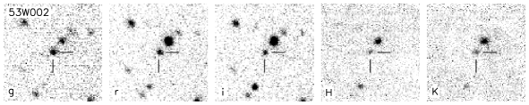
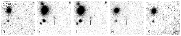
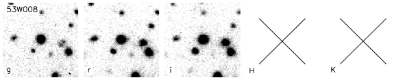
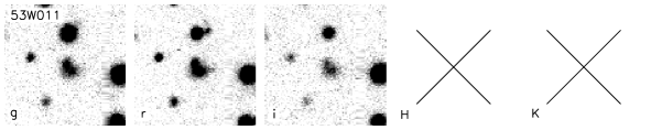
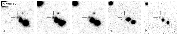
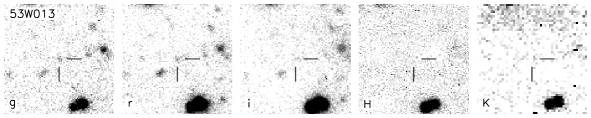
Figure 5: $griHK$ images (from left to right) for those sources in the LBDS Hercules sample that were identified on the optical CCD images discussed in section 3. Only three of these sources (53W002, 53W069, & 53W091) had $J$-band observations which have been published elsewhere. Each image is 30 arcsec on a side, and is orientated with north to the top, east to the left. Crosshairs denote the radio source where necessary.

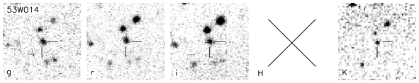
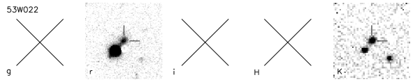
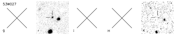
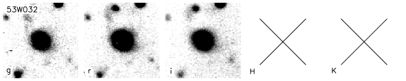
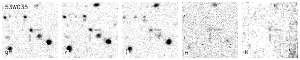
Figure 6: continued

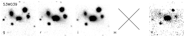
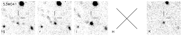
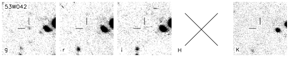
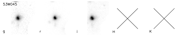
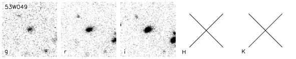
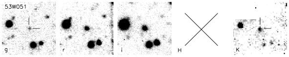
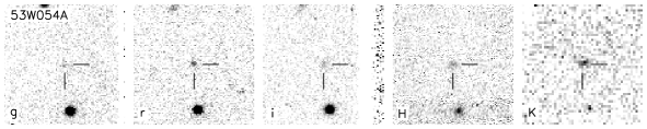
Figure 7: continued

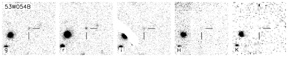
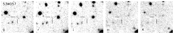
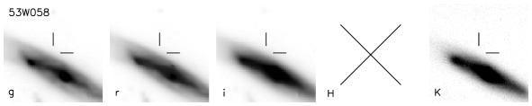
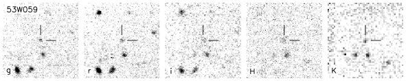
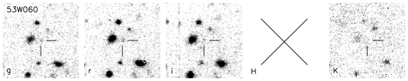
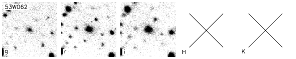
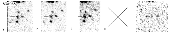
Figure 8: continued

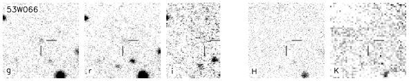
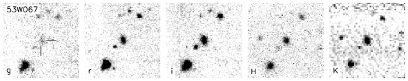
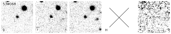
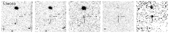
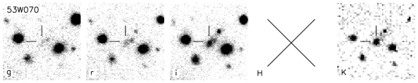
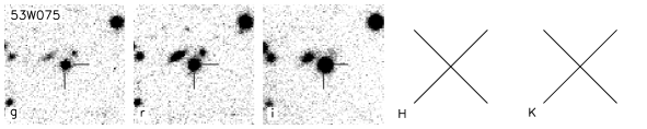
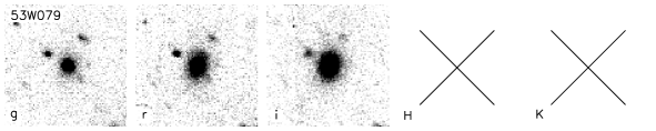
Figure 9: continued

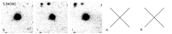
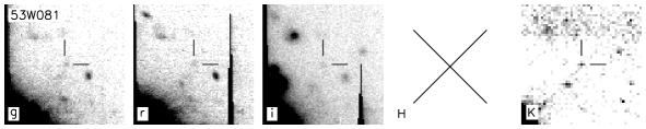
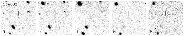
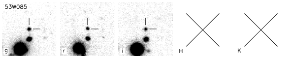
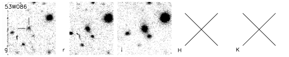
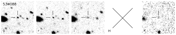
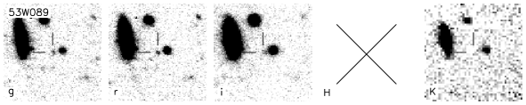
Figure 10: continued

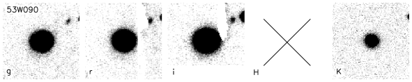
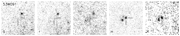
Figure 11: continued

3.4 Photometry

The photometric calibration of the 4-Shooter images was done in two stages, due to the non-photometric conditions of a significant number of the observing nights. For most of the sources, at least one exposure had been taken on a photometric night which could therefore be calibrated accurately. This calibrated exposure was then used to bootstrap a zero-point for the non-photometric mosaic of all the exposures.

The apparent magnitude of a source ($m$) is defined by

$$m=m_{\rm inst}+k\cdot\overline{{\rm sec}z}+C\cdot(g-r)+z_{\rm p}$$ (6)

where $m_{\rm inst}$ is the instrumental magnitude, $k$ is the extinction coefficient for a given filter, $\overline{{\rm sec}z}$ is the time-averaged airmass, $C$ is the colour coefficient for the filter, $(g-r)$ is the instrumental colour of the source, and $z_{\rm p}$ is the zero-point. Higher order terms are not included due to the limited number of standard star observations available.

For each night of the observing runs, there were between three and eight observations of Gunn standard stars made. These were taken throughout the night at different airmasses and in all three filters. To avoid saturation, the standard stars were observed with the telescope out of focus. Instrumental magnitudes in a 30″–40″ circular aperture were measured for each star, on every night that the log sheets recorded as being photometric. True apparent magnitudes ($m_{0}$) were taken from a list of both published and unpublished standards available at the telescope [Thuan & Gunn 1976, Wade et al. 1979, Kent 1985]. Equation 6 was then fitted to the data ($m_{0}-m_{\rm inst}$, ${\rm sec}z$, $g-r$) using a linear least squares method. This gave best-fitting values for $k$, $z_{p}$ and $C$ for each night. The colour coefficients are not expected to change from night to night and the fitted values were indeed consistent, thus a weighted average over all the nights in a run was used. A second least squares fit was then performed with $C$ fixed at its average value, and values for $k$ and $z_{\rm p}$ were found for each photometric night. For the non-photometric mosaics, the extinction and colour coefficients were taken as the mean of the values over all the runs (Table 8). Note that these values are consistent with those assumed by Neuschaefer & Windhorst (1995), who used the same instrument and telescope, over a similar period of time (1984–1988).

For each photometric image containing a radio source, the automated image detection program pisa [Draper & Eaton 1996] was used to calibrate 20–80 sources in the image. The search parameters were chosen such that a source was defined as having at least eight contiguous pixels with values greater than 5-$\sigma$ above the background. Such conservative parameters ensured that only good signal-to-noise sources were detected in the relatively short photometric exposure. The corresponding non-photometric, deep mosaic was then analysed in the same way with pisa. The mean difference in magnitude between each source, as observed in the mosaic and in the calibrated exposure, then allowed the zero-point of the non-photometric mosaic to be bootstrapped from the calibrated photometric image.

Table 8: Mean extinction & colour coefficients

Filter	$\overline{k}$	$\overline{C}$
$g$	$-0.28\pm 0.05$	$0.16\pm 0.02$
$r$	$-0.14\pm 0.03$	$0.10\pm 0.01$
$i$	$-0.11\pm 0.02$	$0.05\pm 0.01$

For five sources (53W010, 53W019, 53W020, 53W022, 53W027), only $r$-band observations from the 1984 run were available so no colour correction could be applied to them. In addition, only two standard star observations were available for each of the two nights, which was inadequate to determine both the extinction and zero-points. Thus, the mean extinction coefficient from Table 8 was adopted, and the zero-point calculated from the observed magnitudes of the standards. For five other sources (53W080, 53W081, 53W085, 53W086, 53W090), no photometric calibrations were available for the $g$ and $r$ images. The zero-points adopted for these mosaics were taken as the mean of the zero-points for all the other observations in the sample. This is reflected in the slightly larger errors for these sources in Table 5.

The sky background subtraction for each source was done using a method based upon the image reduction package cassandra by D. P. Schneider, adapted to run as an iraf task using the apphot package for the numerical work. A rectangular box (typically 10″–20″ on a side) surrounding the source, and excluding any other objects, was cut out of the mosaic image. A plane was fitted to this box, excluding from the fit a circle centered on the source, and the sky was subtracted from the image. Photometry was performed using a circular aperture of 4$\aas@@fstack{\prime\prime}$0, 7$\aas@@fstack{\prime\prime}$5 or 10$\aas@@fstack{\prime\prime}$0 diameter (depending on the extent of the source), with the sky statistics determined over the remainder of the box. This enabled a large asymmetric sky aperture to be used, which is not possible with the basic apphot, in addition to providing a better measure of the sky background than is possible with an annulus around the object.

During testing of this method an error was found in the way that apphot calculates magnitude errors for faint objects. apphot makes the approximation $\ln(1+\Delta)\approx\Delta$ which for faint sources overestimates the error by as much as 0.1–0.2 magnitudes. This was corrected by including the second, and for good measure the third, order terms in the expansion: $\ln(1+\Delta)\approx\Delta-\Delta^{2}/2+{\Delta^{3}/3}$. The apparent magnitude was then calculated from equation 6 using the coefficients in Table 8 and the appropriate zero-points. The results are presented in Table 5. The errors quoted are the quadratic sum of the instrumental magnitude errors from apphot (shot-noise in the object aperture, sky-noise), and the errors in the determination of $k$, $C$ and $z_{\rm p}$.

Figure 12: Accuracy of the photometric transformations from $J^{+}F^{+}N^{+}$ to $gri$ for the eighteen sources with measurements in both systems. $g_{\rm trans}$, $r_{\rm trans}$ and $i_{\rm trans}$ are the photographic magnitudes transformed to the Gunn system with equations 7–9, $g$, $r$ and $i$ are the observed 4-Shooter magnitudes.

In order to compare those radio sources with photographic magnitudes, $J^{+}F^{+}N^{+}$, to those sources with 4-Shooter Gunn magnitudes, $gri$, it was necessary to convert one photometric system to another [Fukugita, Shimasaku & Ichikawa 1995]. Windhorst et al. (1991) derived transformations from the Gunn system to the photographic system, and inverting these gives the required equations:

$$g = 0.69{J^{+}}+0.31{F^{+}}-0.19$$ (7)

$$r = 1.14{F^{+}}-0.14{J^{+}}+0.34$$ (8)

$$i = {N^{+}}+0.75$$ (9)

For those sources without 4-Shooter observations, the optical magnitudes in Table 5 are photographic magnitudes from Kron et al. (1985) transformed to the Gunn system using these equations. An error of 0.3 magnitudes is assigned to each of these values, corresponding to the quadratic sum of the error in the transformations (0.1 mag) and the error in the photographic magnitudes (0.2–0.3 mag). For the eighteen sources with both photographic and 4-Shooter Gunn photometry, the transformed photographic magnitudes are compared with the 4-Shooter data in Fig. 12. It can be seen that the transformations are in good agreement with the data for $gri\la 22$–23 mag; fainter than this, the $J^{+}F^{+}N^{+}$ magnitudes are close to the detection limits of the photographic plates and are less reliable.

4 Infrared photometry

Infrared data are crucial to understanding high-redshift galaxies. Beyond $z\sim 1$, optical observations sample the restframe ultraviolet emission of galaxies and the restframe optical emission has shifted into the near-infrared. Thus in order to properly compare sources at high-$z$ with those at low-$z$, the analysis must move to longer wavelengths. The $K$-band has long been recognized as a valuable window through which to investigate radio galaxies, and so we sought to obtain $K$ magnitudes for the complete Hercules sample.

4.1 Observations with the UK Infrared Telescope

Approximately half the sample has been observed during three major observing runs at the 3.8-m UK Infrared Telescope, Mauna Kea, Hawaii (Table 4). The first two runs (1992 & 1993) used the infrared camera IRCAM, a 62$\times$58-pixel InSb array with a scale of 0.62 arcsec pixel^-1. All these observations were done in the $K$-band. The 1997 run used the upgraded camera IRCAM3, which had 256$\times$256 pixels with a scale of 0.286 arcsec pixel^-1. Deep $K$ images were obtained for sources which had not previously been detected, together with $H$-band observations of several galaxies for which $H$ was considered important for constraining the redshift. Additional observations of some sources were made during associated projects and via the UKIRT Service Observing programme.

A standard jittering procedure was used to obtain a median-filtered sky flat-field simultaneously with the data. Nine 3-minute exposures were made, each offset by 8″ (1992 & 1993) or 15″ (1997) from the first position, resulting in a central area around the radio source with a maximal exposure time of 27 minutes, surrounded by a border of low signal-to-noise data. This was repeated two or three times for the faintest sources. Observations of faint standard stars were taken to calibrate the data.

4.2 Data reduction and calibration

For all three UKIRT runs, the image processing stage in the reduction was performed at the telescope by the observers. This consisted of the following steps: (i) a dark frame observed prior to the nine-exposure sequence was subtracted from each image; (ii) a normalised flat-field was constructed by taking the median of the nine exposures; (iii) each exposure was then divided by the flat-field; (iv) an extinction correction was applied; (v) the images were registered and finally combined into a mosaic after rejection of known bad pixels.

The standard star observations were reduced in the same manner, and the instrumental magnitude (corrected for extinction) calculated. Comparison with the known apparent magnitude then yielded a zero-point. Standards were observed regularly and the zero-points were found to vary by $<0.05$ mag throughout each photometric night. Colour coefficients are small in the infrared and were not determined.

Photometry was performed on each of the mosaics using the same method as for the optical data (§3.5), with the exception of the 1992 observations for which the sky background was determined from the mean of $\simeq 5$ circular apertures placed randomly around the source. The results are presented in Table 5 and Fig. 5. In addition to the 36 new observations described here, Table 5 contains infrared data published by Thuan et al. (1984) for sixteen sources, unpublished data from G. Neugebauer, P. Katgert et al. (private communications) for a further twenty sources, and data on five other galaxies referenced in the notes to the table.

5 Discussion of the multi-colour photometry

The results of the optical and infrared photometry are discussed in this section, and compared with both earlier results from the LBDS and with results from other radio surveys. Discussion of redshift-dependent properties will be presented in Paper II, following analysis of the new spectroscopic data.

Figure 13: Magnitude distributions for the three optical bands ($g$, $r$, $i$). Shaded histograms show the 2-mJy sample data, open histograms show the full Hercules data. Photographic magnitudes have been transformed to the Gunn system using equations 7–9. The limits of the photographic data correspond to $g\simeq 23.0$ mag, $r\simeq 22.3$ mag and $i\simeq 21.5$ mag.

Figure 14: Magnitude distributions for the three infrared bands ($J$, $H$, $K$). Shaded histograms show the 2-mJy sample data, open histograms show the full Hercules data. Arrows denote 3-$\sigma$ upper limits.

5.1 Notes on individual sources

Before investigating the photometric properties of the sample as a whole, the optical, infrared & radio observations of some individual sources are worth noting.

53W002 – This $z=2.390$ radio galaxy has been the subject of much study (see §2.1). Comparing the optical and infrared colours recorded in Windhorst et al. (1991) with those here, shows that they are fully consistent within the errors, although there is some discrepancy between the optical magnitudes. This may be explained by noting that Windhorst et al. use “total” magnitudes which are brighter than the 4″ aperture magnitudes in Table 5 – indeed, application of the same method to these data produces consistent results. It is important to note that the colours of faint sources are not significantly affected by aperture size so long as the aperture is larger than the seeing disk, which it is in all cases here.

53W011 & 53W013 – There was originally some concern that these two sources may have been confused with the grating rings in the WSRT observations, however both have optical counterparts and so are retained in the sample.

53W014 – Optical counterpart is at 3.1-$\sigma$ from the radio position. A second object, 5″ to the north-east, at 3.7-$\sigma$, may also be a possible identification.

53W022 – New identification compared with Windhorst et al. (1984b). This object looks as if it could be physically associated with the brighter old identification in the $r$-band. At $K$, the two objects are distinct and very similar in appearance.

53W032 – A $z=0.370$ galaxy at the centroid of a double radio source. The 4-Shooter images reveal extended emission to the north-east, reminiscent of a tidal tail. Note also that component A is coincident with an $r\simeq 20.3$ mag source, although component B does not have an optical counterpart.

53W035 & 53W089 – These sources each appeared on two independent mosaics, enabling the repeatability of the photometry to be confirmed.

53W054A & 53W054B – Originally classified as the lobes of a classical double radio source [Windhorst et al. 1984a], they are now considered to be two distinct sources. Both have solid identifications in the optical, and 53W054A is also identified in the infrared.

53W057 – $K$ is a marginal (2-$\sigma$) detection at the north-east end of the elongated source in $g$. The brighter source at 6″ to the west is also a possible identification, at 2-$\sigma$ from the radio position.

53W058 – The radio source is in the arm of a bright spiral galaxy at $z=0.034$. The coordinates given in Table 5 are for the centre of the galaxy; the position of the radio emission is marked in Fig. 5.

53W067 – The optical counterpart is 4$\aas@@fstack{\prime\prime}$8 (8-$\sigma$) from the radio position but has [Oii] and Ca H & K lines identified in the spectrum, at a redshift of 0.759 (Paper II). The fainter source to the south-east, originally proposed as the identification (at a separation of 1.2-$\sigma$), was identified as an M-type star from spectroscopy with the Keck telescope (Spinrad, Dey & Stern, 1997, private communication).

53W069 & 53W091 – These two red sources at $z\simeq 1.5$ have been extensively studied with both the Keck Telescope and the Hubble Space Telescope. Their rest-frame ultraviolet spectra are consistent with an evolved stellar population of ages 3–4 Gyr [Dey 1997, Dunlop et al. 1996, Dunlop 1999, Spinrad et al. 1997], and their rest-frame optical morphologies are dominated by $r^{1/4}$ elliptical profiles [Waddington et al. 2000b].

5.2 General properties of the sample

The apparent magnitude distribution is of cosmological interest because it is closely related to the radio source redshift distribution. Broadly speaking, the fainter a source is (in optical/infrared wavebands), the more distant it is expected to be. Although complicated by evolutionary effects, in the absence of spectroscopic data the magnitude distribution has been an important tool in studying radio galaxies.

The optical data are shown in Fig. 13 and the infrared data in Fig. 14. In addition to the full Hercules distributions, the 2-mJy sample is shown as hatched histograms. The first issue that is apparent from these figures is the greater depth of the new observations. The limiting magnitudes of the Kron et al. (1985) photographic data correspond to $g\simeq 23.0$ mag, $r\simeq 22.3$ mag and $i\simeq 21.5$ mag. The 4-Shooter data extend some 3–4 magnitudes fainter in all passbands. The infrared $K$-band data are similarly about four magnitudes deeper than the Thuan et al. (1984) results. The $griK$ data are essential complete, approximately half the sources have $H$-band measurements and only one-third of the sample has been observed in $J$.

It is clear from Figs. 13 & 14 that the number of galaxies per magnitude interval does not continue to increase down to the magnitude limit, but rather turns over at $r\sim 22$ mag. This immediately points to evolution of some form in the radio source population – if the radio sources formed an homogeneous class of object present throughout the history of the universe, the numbers would continue to increase towards the magnitude limit. This turnover was hinted at in the $N^{+}$ magnitude distribution of the whole LBDS [Windhorst et al. 1984b] and is clearly confirmed for the Hercules subsample here. Excluding the 1 mJy $\leq S_{1.4}<2$ mJy sources does not significantly change the shape of the magnitude distributions, but it does increase the median magnitude – i.e. the faintest radio sources are not in general the faintest sources at optical/infrared wavelengths. This would suggest that the faintest radio sources are lower (radio) luminosity objects at lower redshift, rather than radio-powerful objects at high redshift. Some caution must be applied to this conclusion however, given that these sources are few in number (9) but have large weights ($\ga$2.5).

Figure 15: Comparison of the $K$-band magnitude distributions for the LBDS Hercules ($S_{\nu}\geq 0.001$ Jy at 1.4 GHz), PSR ($S_{\nu}\geq 0.1$ Jy at 2.7 GHz), 1-Jansky ($S_{\nu}\geq 1$ Jy at 0.408 GHz) and 3CR ($S_{\nu}\geq 10$ Jy at 0.178 GHz) samples. Open histograms are the galaxies and uncertain IDs (G, G? or ?), hatched histograms are the quasars (Q or Q?), and the shaded histogram in the top panel is the 2-mJy Hercules sample (note that all the LBDS quasars have $S_{1.4}\geq 2$ mJy).

In Fig. 15, the LBDS $K$-band magnitude distribution is compared with the results of three other radio samples with near complete infrared data. The Parkes Selected Regions (PSR) data are principally taken from Dunlop et al. (1989). Only sources in their four-region subsample, for which the $K$-band data are essentially complete, are used (the 12^h and 13^h regions are poorly covered in the infrared). The 1-Jansky sample of Allington-Smith (1982) is a complete sample of 59 radio sources with 1 Jy $<S_{\nu}<2$ Jy at 408 MHz. Lilly, Longair & Allington-Smith (1985) presented infrared observations of 53 of these sources, which are plotted in the third panel of Fig. 15. Finally, a complete sample of 90 radio galaxies was selected from the 173-source 3CR catalogue of Laing, Riley & Longair (1983). Nearly complete $K$-band data was obtained for this 3CR sub-sample [Lilly & Longair 1984], which excludes all quasars, and is shown in the last panel of the figure. For the first three samples, both galaxies and quasars are shown. The LBDS panel also includes the 2-mJy sample for comparison.

Figure 16: Colour–magnitude diagrams for the LBDS Hercules sample. Solid circles denote galaxies (G, G? or ? types) in the 2-mJy sample. Open circles denote galaxies with 1 mJy $\leq S_{1.4}<2$ mJy. Triangles denote quasars (Q or Q?), all of which have $S_{1.4}\geq 2$ mJy. Dashed lines show the completeness limits of the photometry. The $J$ and $H$ data are not complete to any apparent magnitude, thus no limits are plotted in (c), (d) and (e).

As first pointed out by Dunlop et al. (1989), the 1-Jansky radio galaxies are biased towards larger $K$ magnitudes than the (radio) brighter 3CR galaxies. However, a similar shift is not seen between the 1-Jansky and PSR sources, a further factor of two fainter in flux. Dropping another factor of $\sim$200 in flux, the LBDS galaxies are seen here to have much the same distribution as the 1-Jansky and PSR galaxies. The median $K$ magnitudes for the four samples are 15.3 (3CR), 16.5 (1-Jy), 16.5 (PSR) and 16.8 (LBDS). To the extent that the $K$ magnitude of a powerful radio galaxy is a good estimator of its redshift, this result implies that although the 1-Jansky galaxies are consistent with being high-redshift counterparts of the 3CR galaxies, these same sources are not seen at even higher redshifts in the fainter samples. (Note that a median spectral index of $\alpha=0.8$ was used to bring the flux limits of the samples to a common frequency for this comparison.)

Although the number of sources is small, the same effect is not seen in the quasar distributions. The median $K$ magnitude of quasars in the fainter three samples increases with decreasing flux limit: 16.1 (1-Jy), 16.3 (PSR) and 16.8 (LBDS). This may suggest that the quasar population is not changing as rapidly as the radio galaxy population. It must be noted, however, that the decrease in restframe optical/infrared flux between the 1-Jansky and LBDS quasars (a factor of $\sim 2$) is certainly not comparable to the drop in radio flux (a factor of $\sim 400$) – i.e. if the $K$ magnitude is a fair redshift estimator, the LBDS quasars must be less luminous in the radio than the 1-Jansky quasars.

Fig. 16 presents colour–magnitude diagrams for the Hercules sample. To compare these results with those of Kron et al. (1985), note that the colours are related by $(g-r)\sim(J^{+}-F^{+})-0.5$ and $(r-i)\sim(F^{+}-N^{+})-0.4$ (from equations 7–9). It can be seen that the colours of the new identifications are comparable to those of the photographic identifications at $r\la 22$ mag. There is some bias towards bluer $g-r$ (and to a lesser extent, $r-i$) colours at the fainter magnitudes. In particular, there is a deficit of faint ($r>23$ mag), red ($g-r>0.5$, $r-i>1$) radio sources compared with field galaxy surveys of comparable depth [Neuschaefer 1992, Neuschaefer & Windhorst 1995]. This is consistent with a continuation of the faint blue radio galaxy population that Kron et al. (1985) found at brighter magnitudes.

The sources classified as quasars (Q & Q?) tend to have bluer optical colours on average than the galaxies, as one would expect from the dominance of the AGN at ultraviolet/optical wavelengths in such sources. (Recall that the classification was based on morphology, not colour.) The “galaxy” class includes objects of unknown identity (?), which dominate at the faintest magnitudes. Figs. 16(a), (b) & (f) suggest that the bluest of these objects may in fact be quasars. Fig. 6 of Dunlop et al. (1989) shows that essentially all PSR sources with $K\ga 15$ and $R-K\la 3$ are quasars. Comparing that figure with Fig. 16(f) here, shows that the same cannot be said for the LBDS – only one of these faint blue objects is of uncertain classification (53W068) and one is a probable quasar (53W036), while the other three are G (53W034, 53W067) and G? (53W027). The LBDS quasars have a much broader range of colours than those in the PSR, perhaps a consequence of their weaker AGN.

Figs. 16(c), (d) & (e) show the distribution of near-infrared colours with apparent magnitude. In considering these figures, it must be remembered how incomplete these data are (only one-third of the sample has $J$-band data, only one-half has been observed in the $H$-band). There appears to be a linear correlation between $i-J$ colour and $i$ magnitude in Fig. 16(c), however this may simply be due to the absence of faint $J$-band photometry – at any given $i$ magnitude it is the reddest sources in the sample that would have been preferentially detected at $J$. The dispersion of the $J-H$ colours (0.2 mag), defined as the standard deviation about the mean colour, is 2–3 times smaller than the dispersion in the optical colours. This is probably due to the incomplete infrared data, but may also be a genuine property of the sample. The smaller scatter may indicate that the infrared emission is dominated by stellar light from the host galaxies, rather than emission from the AGN which tends to dominate at bluer wavelengths and can vary significantly from one source to another.

To summarize, the optical identification of the 72-source LBDS Hercules sample is essentially complete (only three sources remain unidentified). Approximately 85% of the sources have also been identified in the near-infrared $K$-band and a programme to obtain complete $J$- and $H$-band data is ongoing. Paper II will present the results of work to measure redshifts for this sample from both direct spectroscopy and by using photometric estimation techniques. This is now the most comprehensive sample of radio-selected sources available at millijansky flux density levels, and is ideally suited to study the evolution of the 1.4 GHz radio luminosity function (for AGN) out to very high redshifts – a topic to be addressed in forthcoming papers.

References

- [Allington-Smith 1982] Allington-Smith J. R., 1982, MNRAS, 199, 611
- [Becker at al. 1995] Becker R. H., White R. L., Helfand D. J., 1995, ApJ, 450, 559
- [Best et al. 1996] Best P. N., Longair M. S., Röttgering H. J. A., 1996, MNRAS, 280, L9
- [Best et al. 1997] Best P. N., Longair M. S., Röttgering H. J. A., 1997, MNRAS, 292, 758
- [Bruzual & Magris 1997] Bruzual G. A., Magris G. C., 1997, in Waller W. H., Fanelli M. N., Hollis J. E., Danks A. C., eds, The Ultraviolet Universe at Low and High Redshift. American Institute of Physics, Woodbury, p. 291
- [Ciliegi et al. 1999] Ciliegi P. et al., 1999, MNRAS, 302, 222
- [Condon et al. 1998] Condon J. J., Cotton W. D., Greisen E. W., Yin Q. F., Perley R. A., Taylor G. B., Broderick J. J., 1998, AJ, 115, 1693
- [Dey 1997] Dey A., 1997, in Tanvir N., Aragón-Salamanca A., Wall J. V., eds, The Hubble Space Telescope and the High Redshift Universe. World Scientific, Singapore, p. 373
- [Donnelly et al. 1987] Donnelly R. H., Partridge R. B., Windhorst R. A., 1987, ApJ, 321, 94
- [Draper & Eaton 1996] Draper P. W., Eaton N., 1996, PISA – Position Intensity and Shape Analysis (SUN/109.8). Starlink Project, Rutherford Appleton Laboratory
- [Dunlop 1999] Dunlop J. S., 1999, in Röttgering H. J. A., Best P. N., Lehnert M. D., eds, The Most Distant Radio Galaxies. Koninklijke Nederlandse Akademie van Wetenschappen, Amsterdam, p. 71
- [Dunlop & Peacock 1993] Dunlop J. S., Peacock J. A., 1993, MNRAS, 263, 936
- [Dunlop et al. 1989] Dunlop J. S., Peacock J. A., Savage A., Lilly S. J., Heasley J. N., Simon A. J. B., 1989, MNRAS, 238, 1171
- [Dunlop et al. 1996] Dunlop J. S., Peacock J. A., Spinrad H., Dey A., Jimenez R., Stern D., Windhorst R. A., 1996, Nat, 381, 581
- [Fukugita, Shimasaku & Ichikawa 1995] Fukugita M., Shimasaku K., Ichikawa T., 1995, PASP, 107, 945
- [Gruppioni et al. 1997] Gruppioni C., Zamorani G., de Ruiter H. R., Parma P., Mignoli M., Lari C., 1997, MNRAS, 286, 470
- [Gunn et al. 1987] Gunn J. E. et al., 1987, Optical Engineering, 26, 779
- [Hall et al. 1996] Hall P. B., Osmer P. S., Green R. F., Porter A. C., Warren S. J., 1996, ApJ, 462, 614
- [Hopkins et al. 2000] Hopkins A., Windhorst R., Cram L., Ekers R., 2000, PASA, submitted (astro-ph/9906469)
- [Keel & Windhorst 1993] Keel W. C., Windhorst R. A., 1993, AJ, 106, 455
- [Kent 1985] Kent S. M., 1985, PASP, 97, 165
- [Koo & Kron 1982] Koo D. C., Kron R. G., 1982, A&A, 105, 107
- [Kron 1980] Kron R. G., 1980, ApJS, 43, 305
- [Kron et al. 1985] Kron R. G., Koo D. C., Windhorst R. A., 1985, A&A, 146, 38
- [Laing et al. 1983] Laing R. A., Riley J. M., Longair M. S., 1983, MNRAS, 204, 151
- [Lewis & Irwin 1997] Lewis G., Irwin M., 1997, Spectrum: Newsletter of the Royal Greenwich Observatory, Royal Observatory Edinburgh, and the Isaac Newton Group, La Palma, 12, 22
- [Lilly & Longair 1984] Lilly S. J., Longair M. S., 1984, MNRAS, 211, 833
- [Lilly et al. 1985] Lilly S. J., Longair M. S., Allington-Smith J. R., 1985, MNRAS, 215, 37
- [McCarthy et al. 1987] McCarthy P. J., van Breugel W. J. M., Spinrad H., Djorgovski S. G., 1987, ApJ, 321, L29
- [Neuschaefer 1992] Neuschaefer L. W., 1992, PhD Thesis, Arizona State University
- [Neuschaefer & Windhorst 1995] Neuschaefer L. W., Windhorst R. A., 1995, ApJS, 96, 371
- [Oort 1988] Oort M. J. A., 1988, A&A, 193, 5
- [Oort et al. 1987] Oort M. J. A., Katgert P., Steeman F. W. M., Windhorst R. A., 1987, A&A, 179, 41
- [Oort et al. 1988] Oort M. J. A., Steemers W. J. G., Windhorst R. A., 1988, A&AS, 73, 103
- [Pascarelle et al. 1996a] Pascarelle S. M., Windhorst R. A., Driver S. P., Ostrander E. J., Keel W. C., 1996a, ApJ, 456, L21
- [Pascarelle et al. 1996b] Pascarelle S. M., Windhorst R. A., Keel W. C., Odewahn S. C., 1996b, Nat, 383, 45
- [Spinrad et al. 1997] Spinrad H., Dey A., Stern D., Dunlop J. S., Peacock J. A., Jimenez R., Windhorst R. A., 1997, ApJ, 484, 581
- [Steidel et al. 1996] Steidel C. C., Giavalisco M., Pettini M., Dickinson M., Adelberger K. L., 1996, ApJ, 462, L17
- [Steidel et al. 1999] Steidel C. C., Adelberger K. L., Giavalisco M., Dickinson M., Pettini M., 1999, ApJ, 519, 1
- [Tadhunter et al. 1992] Tadhunter C. N., Scarrott S. M., Draper P., Rolph C., 1992, MNRAS, 256, 53p
- [Thuan & Gunn 1976] Thuan T. X., Gunn J. E., 1976, PASP, 88, 543
- [Thuan et al. 1984] Thuan T. X., Windhorst R. A., Puschell J. J., Isaacman R. B., Owen F. N., 1984, ApJ, 285, 515
- [Waddington 1998] Waddington I., 1998, in D’Odorico S., Fontana A., Giallongo E., eds, ASP Conference Series 146, The Young Universe: Galaxy Formation and Evolution at Intermediate and High Redshift. Astronomical Society of the Pacific, San Francisco, p. 520
- [Waddington et al. 1999a] Waddington I., Windhorst R. A., Cohen S. H., Partridge R. B., Spinrad H., Stern D., 1999, ApJ, 526, L77
- [Waddington et al. 2000a] Waddington I., Dunlop J. S., Windhorst R. A., Peacock J. A., 2000a, MNRAS, submitted (Paper II)
- [Waddington et al. 2000b] Waddington I., et al., 2000b, ApJ, in preparation
- [Wade et al. 1979] Wade R. A., Hoessel J. G., Elias J. H., Huchra J. P., 1979, PASP, 91, 35
- [White at al. 1997] White R. L., Becker R. H., Helfand D. J., Gregg M. D., 1997, ApJ, 475, 479
- [Windhorst 1984] Windhorst R. A., 1984, PhD Thesis, University of Leiden
- [Windhorst et al. 1984a] Windhorst R. A., van Heerde G. M., Katgert P., 1984a, A&AS, 58, 1
- [Windhorst et al. 1984b] Windhorst R. A., Kron R. G., Koo D. C., 1984b, A&AS, 58, 39
- [Windhorst et al. 1985] Windhorst R. A., Miley G. K., Owen F. N., Kron R. G., Koo D. G., 1985, ApJ, 289, 494
- [Windhorst et al. 1990] Windhorst R. A., Mathis D., Neuschaefer L., 1990, in Kron R. G., ed, ASP Conference Series 10, Evolution of the Universe of Galaxies. Astronomical Society of the Pacific, San Francisco, p. 389
- [Windhorst et al. 1991] Windhorst R. A. et al., 1991, ApJ, 380, 362
- [Windhorst et al. 1993] Windhorst R. A., Fomalont E. B., Partridge R. B., Lowenthal J. D., 1993, ApJ, 405, 498
- [Windhorst et al. 1994] Windhorst R. A., Gordon J. M., Pascarelle S. M., Schmidtke P. C., Keel W. C., Burkey J. M., Dunlop J. S., 1994, ApJ, 435, 577
- [Windhorst et al. 1998] Windhorst R. A., Keel W. C., Pascarelle S. M., 1998, ApJ, 494, L27
- [Windhorst & Waddington 2000] Windhorst R. A., Waddington I., 2000, in Guiderdoni B. et al., eds, The Birth of Galaxies: Proceedings of the Xth Rencontres de Blois, in press
- [Yi et al. 2000] Yi S., Brown T., Heap S., Hubeny I., Landsman W., Lanz T., Sweigart A., 2000, ApJ, 533, 670