Exploring the gravitationally lensed system HE 1104-1805:
Near-IR Spectroscopy

Abstract

A new technique for the spatial deconvolution of spectra is applied to near-IR (0.95 - 2.50 $\mu$) NTT/SOFI spectra of the lensed, radio-quiet quasar HE 1104$-$1805. The continuum of the lensing galaxy is revealed between 1.5 $\mu$ and 2.5 $\mu$. Although the spectrum does not show strong emission features, it is used in combination with previous optical and IR photometry to infer a plausible redshift in the range $0.8<z<1.2$. Modeling of the system shows that the lens is complex, probably composed of the red galaxy seen between the quasar images and a more extended component associated with a galaxy cluster with fairly low velocity dispersion ($\sim$ 575  km s^-1). Unless more constrains can be put on the mass distribution of the cluster, e.g. from deep X-ray observations, HE 1104$-$1805 will not be a good system to determine H₀. We stress that multiply imaged quasars with known time delays might prove more useful as tools for detecting dark mass in distant lenses than for determining cosmological parameters.

The spectra of the two lensed images of the source are of great interest. They show no trace of reddening at the redshift of the lens nor at the redshift of the source. This supports the hypothesis of an elliptical lens. Additionally, the difference between the spectrum of the brightest component and that of a scaled version of the faintest component is a featureless continuum. Broad and narrow emission lines, including the FeII features, are perfectly subtracted. The very good quality of our spectrum makes it possible to fit precisely the optical Fe II feature, taking into account the underlying continuum over a wide wavelength range. HE 1104$-$1805 can be classified as a weak Fe II emitter. Finally, the slope of the continuum in the brightest image is steeper than the continuum in the faintest image and supports the finding by Wisotzki et al. (1993) that the brightest image is microlensed. This is particularly interesting in view of the new source reconstruction methods from multiwavelength photometric monitoring. While HE 1104-1805 does not seem the best target for determining cosmological parameters, it is probably the second most interesting object after Q 2237+0305 (the Einstein cross), in terms of microlensing.

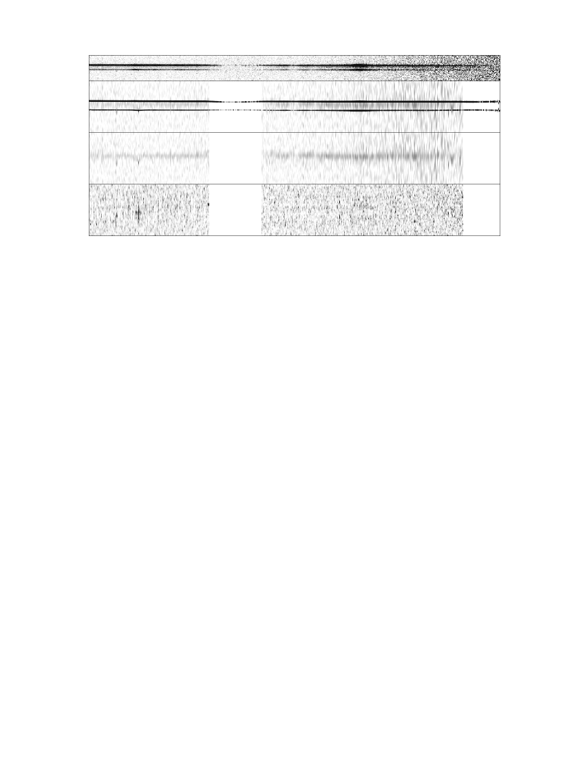
Figure 1: Two dimensional spectra of HE 1104$-$1805. From top to bottom, (i) the 2-D near-IR combined (1.5-2.5 $\mu$) spectrum (seeing $\sim$ 0.6 ″, pixel size $\sim$ 0.14″), (ii) its deconvolved version (resolution of 0.14 ″, pixel size $\sim$ 0.07″), (iii) the deconvolved spectrum of the lens alone, and (iv) the residual map (see text).

1 Introduction

HE 1104$-$1805 is one object in the growing list of gravitationally lensed quasars which might be used to constrain cosmological parameters. It was discovered in the framework of the Hamburg/ESO Quasar Survey and consists of 2 lensed images of a radio-quiet quasar (RQQ) at $z$= 2.319, separated by $\sim$3.15″ (Wisotzki et al. 1993). The lensing galaxy was discovered from ground based near-IR (Courbin, Lidman & Magain, 1998; hereafter C98) and HST optical observations (Remy et al. 1998; hereafter R98). The relatively wide angular separation between the quasar images makes this object suitable for photometric monitoring programs, as conducted at ESO by Wisotzki et al. (1998; hereafter W98). From light curves measured over a period of 6 years, they derived a time delay for HE 1104$-$1805 of $\Delta t=0.73$ years, with a second possible value of 0.3 years. Although we show that the complex lensing potential involved in HE 1104$-$1805 makes it difficult to determine H₀ from the time delay, we also show that HE 1104$-$1805 is probably much more of interest for microlensing studies, provided the lens redshift is better known. The present paper describes an attempt to measure the redshift of the main lensing galaxy from near-IR spectroscopy. Our near-IR observations where motivated by the very red colors measured for the lensing galaxy (C98, R98), and by the better contrast between the lens and the quasar in the near-IR. Although we were unsuccessful in measuring the lens redshift accurately, we did obtain high S/N spectra of the lensed quasar, between 0.95 and 2.5 microns.

2 Observations-Reductions

The data were taken with SOFI, the near-IR (1 to 2.5 $\mu$) imaging spectrograph on the ESO NTT. Two grisms were used to cover the 1 to 2.5 $\mu$ wavelength range: a “blue grism”, which covers the region from 0.95 to 1.64 $\mu$ and a “red grism” which covers the region 1.53 to 2.52 $\mu$. With a 1″  slit, the spectral resolution is around 600. The observations with the blue grism were taken on the night of 1998 June 13, for a total integration time of 4560 seconds and the observations with the red grism were taken on the night of 1999 January 6, with a total integration time of 2400 seconds. Although the seeing for both nights was good, 0.6″  - 0.8″, neither night was photometric.

The slit was aligned with the two images of the quasar. As is standard practice in the infrared, the object was observed at two positions along the slit. The strong and highly variable night sky features were effectively removed by subtracting the resulting spectra from each other. The 2-D sky-subtracted spectra were then flat-fielded, registered, and added.

The two dimensional combined frames were spatially deconvolved in order to extract the spectrum of the lensing galaxy. For this purpose, we used the method outlined by Courbin et al. (1999, 2000). The algorithm is a spectroscopic extension of the so-called “MCS image deconvolution algorithm” (Magain et al. 1998). It spatially deconvolves 2-D spectra of blended objects, using the spectrum of a reference point source. It also improves their spatial sampling and decomposes them into the individual spectra of point sources (the two quasar images) and extended sources (the lensing galaxy). One also obtains a two-dimensional residual map, i.e., the difference between the data and the deconvolved spectrum (reconvolved by the spectrum of the PSF), in units of the photon noise. The quality of the deconvolution is checked using the residual map, which should be flat with a mean value of 1. The different products of the deconvolution are shown in Fig. 1 for the spectrum taken with the red grism.

As the data were obtained before we developed our spectra deconvolution algorithm, we did not observe in an optimal way, in the sense that no reference spectrum was obtained (a spectrum of a star in the field of view). We aligned the slit along the two quasar components, as is usually done for such observations. However, the seeing of the data taken with the red grism was good enough to derive the PSF spectrum from the brighter quasar itself. This was not possible with the data taken with the blue grism.

For the observations taken with the red grism, the spectrum of the lensing galaxy, was extracted from the 2-D deconvolved spectrum (extended component only) with standard aperture extraction techniques. The quasar spectra are a product of the deconvolution process and therefore do not show any contamination by the lensing galaxy. For the observations taken with the blue grism, we used wide apertures to extract the quasar spectra from the original data. The lens is therefore contaminating the spectra of the quasar, but by virtue of its very red color, the contamination is negligible.

All extracted 1-D spectra were then divided by that of a bright star and multiplied by a blackbody curve that has a temperature that is appropriate for the spectral type of the star. Before the division, spectral features that were visible in the spectra of the bright star, such as the Pachen and Bracket lines of hydrogen, were removed by interpolation.

3 Near-IR spectroscopy of the lens

3.1 Plausible lens redshift

The galaxy spectrum is shown in Fig. 2. The signal-to-noise ratio is very low, so the spectrum has been smoothed with a box car with 200 Å  width. Also plotted are the broadband magnitudes of the lens (C98, R98 and Hjorth, private communication). The lens spectrum is scaled to match the $H$ and $K$ band magnitudes.

The spectrum does not lead to a redshift measurement. However, the broadband colours suggest a significant break in the spectrum between the $I$ and $J$ bands. We have used the publicly available photometric redshift code hyperz (Bolzonella, Miralles & Pelló 2000) to estimate the redshift of the lens.

Since there is little evidence for dust in the quasar spectrum (see below), we have fitted dust free models to the data. The best fitting model is a galaxy that was formed in a single burst of star formation. The best fitting redshift is $z=1$ with a 1-sigma range of 0.8 to 1.2. The age of the burst is 1.7 Gyrs. The quoted errors on the redshift do not include systematic errors that could be due to the heterogenous nature of the photometric data, which is derived from a mixture of ground and space based observations.

The estimated redshift is slightly higher than those estimated from the position of the lens on the fundamental plane ($z=0.77\pm 0.07$; Kochanek et al. 2000) or from lens models and the time delay ($z=0.79$; W98). Note however that models including a dark component (see next section) can cope with any redshift between 0.7 and 1.3 and reproduce the observed time delay, assuming for example H${}_{0}=60$ km s^-1 Mpc^-1.

As the break between 0.7 and 1.0 $\mu$ in the model spectra is very strong, a deep spectrum in this region is probably the key to accurately measure its redshift.

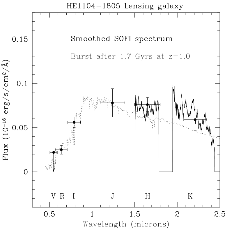
Figure 2: Summary of the spectroscopic and photometric data available for the lensing galaxy in HE 1104$-$1805. Also plotted, is the spectrum of a 1.7 Gyr old burst at z=1.

3.2 Evidence for a high redshift cluster-lens.

With only two quasar images available to constrain the lensing potential, the unusual image configuration of HE 1104$-$1805 (R98) is very difficult to model uniquely. The system can not be reproduced with a Singular Isothermal Sphere. Additional shear and convergence, whatever their origin may be (intrinsic ellipticity of the lens and/or intervening lenses), are required to match simultaneously the positions and flux ratio of the quasar images ($f_{A}/f_{B}$=2.8, see section 4). In a first model, we introduce an ellipticity in the lens model, i.e., we choose an isothermal ellipsoid. Although we can easily obtain a good $\chi^{2}$ fit, the resulting model has a very large velocity dispersion, over 300 km s^-1, and an unrealistic ellipticity compared with the ellipticity of the associated light distribution. Finally, such a model predicts time delays of $470h_{50}$ days, while the observed value is 265 days, according to W98.

The uncertainty on the lens redshift can not explain the discrepancy between the measured and predicted time delays: additional mass is required to describe the image configuration, flux ratio and time delay. We therefore adopt a two component model including (1) the main lensing galaxy, with ellipticity and position angle as constrained by the light distribution of the main galaxy lens, and, (2) a more extended component mimicking an intervening galaxy cluster. For simplicity, we centered the cluster on the main galaxy and assume an elliptical isothermal mass profile with a core radius. The fitted parameters were only the velocity dispersion, the ellipticity and position angle. Both the main lens and cluster components are taken to be at redshift 1.0. Our best fit model is shown in Fig. 3. It involves a cluster with moderate mass, i.e., a velocity dispersion of $\sigma\sim 575\pm 20$ km s^-1. The ellipticity is 0.3 (defined as $e=[1-(a/b)^{2}]/[1+(a/b)^{2}$]) and PA=10  degrees, which is slightly tilted relative to the axis of the main lens (which has PA=46  degrees) and with the light profile of the galaxy visible in the HST images of Lehar et al. (1999), who gives PA=63$\pm$17  degrees). Adding the cluster component also allows one to match better the observed shape parameters of the main lensing galaxy. With the presence of the cluster, the models can accommodate a PA of 46  degrees for the main lensing galaxy and a lower velocity dispersion, $\sigma\sim$ 235 km s^-1.

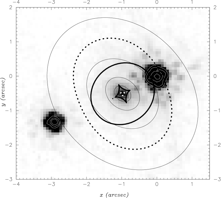
Figure 3: HST-NICMOS2 image of HE 1104$-$1805 (PI: Falco) obtained in the $H$-band, and lens model. The thin solid lines show the isomass density contours for our galaxy$+$cluster lens model. The thick dashed lines are the critical curves and the thick solid lines are the caustic lines at the redshift of the quasar. The dot left to the diamond shape caustic shows the source position for our best fit model.

Figure 4: Total mass within a surface of radius  $r$ for the single galaxy lens model (long dash), galaxy$+$cluster model (solid), and for the galaxy component of the galaxy$+$cluster model (short dash). The positions of the quasar images are marked with vertical lines.

If we assume H${}_{0}=60$ km s^-1 Mpc^-1, $\Omega=0.3$ and $\Lambda=0.7$, the galaxy$+$cluster model reproduces well the measured time delay, giving a value of $\Delta t\sim 265$ days. However, we stress that the lens redshift and the velocity dispersion of the cluster are redundant parameters: increasing the cluster’s mass or decreasing the lens redshift have the same effect on the time delay. This degeneracy between the two parameters will prevent any estimate of H₀ until more observational constraints are available on the cluster component of the lensing matter. The time delay now available in HE 1104$-$1805 can therefore be seen as a new important constraint on the lens model, indicating the presence of a yet undetected cluster, rather than a way to constrain H₀. The mass within an area of a given radius is shown in Fig. 4 for different model components.

If real, the cluster we predict in our model is difficult to detect, with only $\sigma\sim 575\pm 20$ km s^-1. At a redshift of 1, it would be even more difficult to see than the more massive clusters involved in other lenses such as AX J2019+112 (e.g., Benitez et al. 1999) or RX J0911.4+0551 (Burud et al. 1998, Kneib et al. 2000). However the velocity dispersion of such a cluster will change depending on the cluster center position. If it is not aligned with the main galaxy lens, its velocity dispersion will increase significantly. Deep X-ray observations and/or deep IR images of this field would be invaluable in constraining further the models.

4 Near-IR spectroscopy of the source at $z$ = 2.319

The 0.95 - 2.50 $\mu$ spectrum of the quasar pair is shown in Fig. 5. The spectra are on a relative flux scale. Regions of high atmospheric absorption are set to zero. The spectra show clearly the Balmer lines: H$\alpha$, H$\beta$, H$\gamma$ and a partially obscured H$\delta$, the [OIII] doublet and several broad FeII features (Francis et al. 1991). From the Balmer lines, the redshift is 2.323 for the brighter component (component A) and 2.321 for the fainter (component B). The measurement error is $\Delta$z$=0.002$, so the redshift of the two components agree with each other, but are slightly larger than the determination at optical wavelengths ($z=2.317$, Smette et al. 1995). As with most quasars (McIntosh et al. 1999b), the [OIII] doublet is slightly blue shifted ($z=2.319$) with respect to the Balmer lines.

Figure 5: One dimensional near-IR spectra of components A and B of HE 1104$-$1805.

Following Wisotzki et al. (1993), we subtracted a scaled version of the fainter component from the brighter one, that is $f_{\lambda}(A)-c.f_{\lambda}(B)$. The scale is set so that the Balmer lines vanish. We find that we require $c=2.9\pm 0.1$ for the red spectrum and $c=3.0\pm 0.1$ for the blue spectrum. Wisotzki et al. and Smette et al. (1995) have used $c=2.8$. The slight difference between Wisotzki’s value and ours may only reflect systematic differences in the way the object was observed and the way the data were reduced rather than anything real. For example, the IR observations were done with a one-arc-second slit, and any small error in the alignment angle could cause such a difference.

The difference spectra are plotted in Fig. 6. Here we plot the raw difference spectra as the dotted line, and a smoothed version of this as the continuous line. The spectrum of the brighter component is also displayed. The difference spectra are featureless. The residual after subtracting the strong H$\alpha$ line is less than 1%. Not only are the broad hydrogen features removed from the spectra, but the broad iron features and the [OIII] doublet are removed as well. As noted by Wisotzki et al. (1993) there appears to be excess continuum in the brighter component.

Figure 6: Difference spectra of the two quasar images for the blue grism (top) and red grism (bottom). The raw difference spectra are plotted as the dotted lines, a smoothed version of these as the continuous lines. The spectra of the brighter component is also displayed.

4.1 Extinction

The Balmer decrement is around 4 for both components, and this is well within the range expected for unreddened quasars (e.g., Baker et al. 1994). Thus, there is no evidence for absolute reddening. However, the limits we can set on this are weak as the range of values for the Balmer decrement in quasars is rather broad.

The limits for differential reddening are considerably stronger. The ratio of the emission lines in the brighter and fainter components is $2.9\pm 0.1$. The error brackets the measured variation of this ratio over time (six years of observations) and over wavelength. It is not clear if this variation is real or the result of measurement error. This ratio is remarkably constant over a large wavelength range, from CIV at 1549 Å to H$\alpha$, and we can used it to place an upper bound on the amount of differential extinction between the two components. If we assume that the lens is at $z=1$ and if we assume that the standard galactic extinction law (Mathis 1990) is applicable, then the differential extinction between the two components is $\Delta E(B-V)<0.01$ magnitudes.

Recently, Falco et al. (1999) measure a differential extinction of $\Delta E(B-V)=0.07\pm 0.01$ for HE 1104$-$1805 in the sense that the B component has a higher extinction. However, their measurements rely on broad band photometry and their results can be mimicked by chromatic amplification of the continuum region by microlensing. If we were to repeat the experiment by comparing the relative strength of the continuum at 1.25 $\mu$ and 2.15 $\mu$, we would derive a differential extinction of $\Delta E(B-V)=0.16$ magnitudes and we would find also that B component was differentially reddened.

4.2 Emission line properties of the source.

The emission line properties of high redshift quasars have been examined for correlations between line ratios and equivalent widths (McIntosh et al. 1999a,b; Muramaya et al. 1999). As the signal-to-noise ratio and spectral coverage of our IR data are considerably better, we have re-measured the emission line parameters for HE 1104$-$1805.

Figure 7: Left: The top left panel displays the rest-frame spectrum of component A and its fit as described in the text. It is the entire spectrum (multiplied by $1+z_{syst}$), with the model spectrum superposed as a bold line. The lower two left panels are both zooms in the left and right halves of the top panel. The vertical dashed lines are drawn at the rest-frame wavelength of each emission line, considering a systemic redshift of $z_{syst}=2.319$. Right: A zoom in the optical FeII region, again with the fitted spectrum superposed. The bottom panel is the difference between the data and the fit, in units of the photon noise.

Fitting of the spectrum was done in a similar way to that used in McIntosh et al. (1999a), but with extended spectral coverage. The model spectrum is a sum of Gaussian lines superposed on an exponential continuum to which is added a numerical optical FeII template (4250 Å  and 7000 Å). The iron template consists of the optical spectrum of I Zw 1 obtained by Boroson & Green (1992). Before computing the model spectrum the template is smoothed to the resolution of our observations by convolving it with a Gaussian line which has the same FWHM than the broad emission lines of the quasar (CIV, in the present case), i.e., a rest-frame width of 6400 km s^-1, or 14 Å. A systemic redshift of $z_{syst}=2.319$ is determined from the [OIII] $\lambda$5007 emission line and applied to the data to obtain a rest-frame spectrum (multiplied by $1+z_{syst}$ to conserve flux). As the positions of all other emission lines are redshifted relative to the [OIII] line by different amounts, their wavelengths are adjusted independently of each other. We measure a mean redshift of $z_{Balmer}=2.323\pm 0.001$ from the H$\gamma$ $\lambda$4340, H$\beta$ $\lambda$4861, and H$\alpha$ $\lambda$6562 emission lines. We used a sum of Gaussians to fit each Balmer line. This arbitrary decomposition is certainly not aimed at being representative of any physical model but still allows us to measure fluxes. One single Gaussian was used to fit the H$\gamma$ line while two Gaussians are required to fit H$\beta$ and three to fit H$\alpha$ which shows very wide symmetrical wings. The [OIII] doublet is represented by two Gaussians with a fixed line ratio of three (between [OIII] $\lambda$4959 and [OIII] $\lambda$5007). All line widths are fixed during the fit and all intensities are adjusted simultaneously (with the conjugate gradient algorithm) with the strength of the iron template and exponential continuum. The results of the fit are reported in Table 1 and Fig. 7. The best fit spectrum has a power law continuum of the type $F_{\lambda}=\lambda^{-\alpha}$, with $\alpha=3.6$. One-sigma errors were estimated by running the fit with different line widths. In addition to these errors, one should consider the error introduced by the continuum determination. Changing the index of the exponential continuum by 10% can affect iron flux measurement by up to 20%. The other, much narrower emission lines, are less affected, but we stress the need for continuum fitting over a very wide wavelength range in order to minimize such systematic errors. This was pointed out by Murayama et al. (1999). It is now obvious on our better data.

Table 1: Rest-frame emission line properties of HE 1104$-$1805, as measured from the fit performed in section 4.2.

	Flux	FWHM	FWHM	Eq. Width
	(Arbitrary units)	(Å)	km s-1	(Å)
FeII (4434-4685)	1.026 $\pm$ 0.003	$-$	$-$	18.73 $\pm$ 0.07
FeII (4810-5090)	0.608 $\pm$ 0.002	$-$	$-$	14.92 $\pm$ 0.05
H$\beta$ (narrow)	1.283 $\pm$ 0.080	50 $\pm$ 3	3084 $\pm$ 180	$-$
H$\beta$ (broad)	1.922 $\pm$ 0.080	120 $\pm$ 10	7404 $\pm$ 620	$-$
H$\beta$ (total)	3.205 $\pm$ 0.120	$-$	$-$	74 $\pm$ 1
H$\gamma$	1.860 $\pm$ 0.010	80 $\pm$ 3	5528 $\pm$ 210	28 $\pm$ 2
H$\alpha$ (narrow)	0.747 $\pm$ 0.200	30 $\pm$ 3	1370 $\pm$ 140	$-$
H$\alpha$ (medium)	8.739 $\pm$ 0.030	90 $\pm$ 3	4110 $\pm$ 140	$-$
H$\alpha$ (broad)	13.49 $\pm$ 0.030	600 $\pm$ 30	27400 $\pm$ 1400	$-$
H$\alpha$ (total)	22.97 $\pm$ 0.210	$-$	$-$	1563 $\pm$ 15
OIII (4959)	0.194 $\pm$ 0.010	25 $\pm$ 2	1512 $\pm$ 120	$-$
OIII (5077)	0.581 $\pm$ 0.030	25 $\pm$ 2	1496 $\pm$ 120	14.8 $\pm$ 0.7

The quality of the fit is overall very good; however, there are some regions where significant differences exist, as indicated by the residuals shown in the bottom left panel of Fig. 7. Most notably the FeII complex red-wards of [OIII] is relatively stronger that the FeII complex blue-wards of H$\beta$.

The ratio of the EWs of [FeII] to H$\beta$ is 0.20. This is slightly lower than that measured by McIntosh et al. (1999a), who report 0.29${}^{+0.07}_{-0.09}$. The difference is probably not significant but there are two systematic biases that make a direct comparison difficult. Firstly, the continuum in this fit is well determined, whereas the small spectral coverage of the previous work may mean that EWs are underestimated (Muramaya et al. 1999). Secondly, and more fundamentally, EWs measured in lensed quasars are susceptible to microlensing which preferentially amplifies the continuum rather than the larger emission line regions. In fact, the continuum for unlensed quasars also varies. This means that EWs are a poor measure to use. Line fluxes are not susceptible to continuum variations, no matter how the continuum varies, whether it is intrinsic to the AGN or caused by microlensing. From our fit, we measure F(FeII(4810-5090)) / F(H$\beta$) = 0.18 $\pm$ 0.04 and F(FeII(4434-4685)) / F(H$\beta$) = 0.32 $\pm$ 0.04 which, according to Lipari et al. (1993) makes of HE 1104$-$1805 a rather weak FeII emitter.

5 Is microlensing detected in HE 1104$-$1805 ?

The possibility of microlensing can be judged from a comparison between the size of the Einstein ring and the size of a quasar continuum emitting region. The latter is thought to be produced by an accretion disk and is of the order of $10^{14}$ to $3\times 10^{15}$ cm (Wambsganss et al. 1990; Krolik 1999 and references therein). The former depends on the mass of the microlenses, $M$, and is $3.0\times 10^{16}\sqrt{(}M/M_{\odot})$ cm. In this calculation and those that follow, we have assumed that the lens is at $z=1$, and we have assumed a cosmology where $H_{0}=60$ km s^-1 Mpc^-1, and $(\Omega_{M},\Omega_{\Lambda})=(0.3,0.0)$. Thus, given that there is a suitable alignment, microlensing of the continuum is possible. Furthermore, the spectrum of the A component is considerably harder than that of the B component. This chromatic effect supports the idea that the continuum is microlensed since higher energy photons come from the inner part of the accretion disk, and are hence more susceptible to high amplification microlensing than lower energy photons. In fact, with suitable modeling of the lens and additional spectroscopic data, it may be possible to place constraints on accretion disc models (e.g., Agol & Krolik, 1999).

The likelihood of microlensing then depends on the density of micro-lenses. If we model the mass distribution of the lensing galaxy as in section $3.2$, we can use the distance between the two macro images to determine the mass density at each image position. This gravitational convergence or optical depth, $\kappa$, is quite high for both components. For the A component, it is $\kappa=0.73$; for the B component, it is 0.53. If this is made entirely of stars then microlensing of either component is highly likely. In detail, however, only the main lensing galaxy is contributing to microlensing. The actual microlensing optical depth at the two quasar image positions is then lower, but still high.

The typical time-scale between two consecutive microlensing events depends on the transverse velocity of the source and the velocity dispersion of the microlenses. The velocity dispersion for the lensing galaxy is high (using a single galaxy model one derives $\sigma\approx 300$ km s^-1, or about 235 km s^-1 if a cluster is also involved) and it is probably larger than the transverse bulk velocity. Dividing this velocity directly by the diameter of the Einstein ring, one derives a time scale of 3 years. This is quite long; however, it has been shown that stellar proper motions produce a higher microlensing rate than the one produced by a bulk velocity of the same magnitude (Wambsganss and Kundic 1995, Wyithe et al. 2000). Furthermore, the typical duration of a microlensing event is the time for the continuum emitting region ($10^{15}\rm cm$) to cross a caustic with velocity $\sigma\approx 300$ km s^-1. This is of the order of a few months and much shorter that the time between consecutive microlensing events.

Thus, it is likely that microlensing affects the A component. As the stellar density of the lens near the B component is approximately half that of the A component, it is quite likely that microlensing affects the B component as well. We should expect that the continuum of the A component should be preferentially amplified relative to that of the B component for the majority of the time, but we should also expect that the B component should be preferentially amplified for a fraction of the time. HE 1104$-$1805 has now been monitored spectroscopically for six years (Wisotzki et al. 1998). During that time, the continuum of both components have been observed to vary; however, the continuum of the A component has always been harder (Wisotzki, private communication). As the time delay between the two components is of the order of 0.73 year (W98), the hardness of the continuum in the A component cannot be attributed to time delay effects. The most natural explanation is microlensing.

Additionally, the relative level of the continuum of the A component is more variable than that of the B component (see Fig. 2 in W98). This cannot be attributed to photometric errors, because the A component is a factor of 3 brighter than B, both components are well separated and the lensing galaxy is much fainter than either component.

Conversely, the BLR does not appear to be affected by microlensing. From 1993 to 1999, the ratio of the broad lines between the two components has varied little, with $2.9\leavevmode\nobreak\ \pm\leavevmode\nobreak\ 0.1$ (W98 and this paper).

The lines of the BLR in the IR spectra presented here subtract very cleanly, better than 1% of the original line flux. Naively, one may then expect that any substructure in the BLR needs to be considerably larger than the microlensing caustics, i.e., $3\times 10^{16}$ cm. However, a more secure estimate requires better modeling of how microlensing in this particular lens can affect the profile of lines from the BLR (e.g., Schneider & Wambsganss, 1990).

6 Conclusions

We have obtained 1 $\mu$ - 2.5 $\mu$ spectra of the gravitational lens HE 1104$-$1805. Although we were not successful in measuring a precise redshift for the lens, the lens is probably an early type galaxy with a plausible redshift of $0.8<z<1.2$. This is slightly larger than estimates based on the measured time delay and estimates based from the position of the lens on the fundamental plane. We show however, that we can reconcile time delay and lens redshift by adding a cluster component to the lens models.

We find that the continuum in the A component is harder than the continuum in the B component. The most probable explanation is that the A component is microlensed by compact objects in the lens galaxy.

The ratio of the emission lines between the two components is $2.9\pm 0.1$. This is consistent with that measured at optical wavelengths. The constancy of this ratio over a large wavelength range limits strongly the amount of differential extinction between the two components. We find that the differential extinction is $\Delta E(B-V)<0.01$ magnitudes.

We find that broad and narrow emission lines can be removed very well by subtracting a scaled version of the spectrum of component B from the spectrum of component A. The residual near the $H\alpha$ line is less than $1\%$ of the original line flux. It may be possible to use this near perfect subtraction to limit models of the BLR. This possibility should be investigated further.

Finally, we note that the time delay measured in HE 1104$-$1805 allows us to demonstrate that the lensing potential is composed of a main lensing galaxy and a more extended “cluster” component. Without the time delay a single galaxy lens would also have been a viable model. With the rapidly increasing number of lenses with known time delay, we can therefore expect to constrain the content in dark matter of lens galaxies and it may be found that intervening clusters are a lot more frequent than first thought.

- (1) Agol E., Krolik J., 1999, ApJ 524, 49
- (2) Baker A. C., Carswell R. F., Bailey J. A. et al. 1994, MNRAS 270, 575
- (3) Benitez N., Broadhurst T., Rosati P., et al. 1999, ApJ 527, 31
- (4) Bolzonella M., Miralles J. M., Pelló R., 2000, astro-ph/0003380
- (5) Boroson T.A., Green R.F., 1992, ApJS 80, 109
- (6) Burud I., Courbin F., Lidman C., et al. 1998, ApJ 501, L5
- (7) Courbin F., Lidman C., Magain P., 1998, A&A 330, 57
- (8) Courbin F., Magain P., Sohy S., Lidman C., Meylan G., 1999, ESO-Messenger 97, 26
- (9) Courbin F., Magain P., Kirkove M., Sohy S., 2000, ApJ 529, 1136
- (10) Falco E.E., Impey C.D., Kochanek C.S., et al. 1999, ApJ 523, 617
- (11) Francis P. J., Hewett P. C., Foltz, et al. 1991, ApJ 373 465
- (12) Krolik J., 1999 “Active galactic nuclei : from the central black hole to the galactic environment”, Princeton Series in Astrophysics, Princeton University Press, ed. J., P., Ostriker.
- (13) Kochanek C. S, Falco E.E., Impey C. D., et al. 2000, ApJ in press
- (14) Kneib J.-P., Cohen J., Hjorth J., 2000, ApJ submitted
- (15) Lehar J., Falco E., Kochanek C., et al. 1999, astro-ph/9909072
- (16) Lipari S., Terlevisch R., Macchetto F., 1993, ApJ 406, 451
- (17) Magain P., Courbin F., Sohy S., 1998, ApJ 494, 472
- (18) Mathis J. S., 1990, ARA&A 28, 37
- (19) McIntosh D. H., Rieke M. J., Rix H.-W., Foltz C. B., Weymann R. J., 1999a, ApJ 514, 40
- (20) McIntosh D. H., Rix H.-W., Rieke M. J., Foltz C. B., 1999b, ApJ 517, L73
- (21) Murayama T., Taniguchi Y., Evans A., et al. 1999, AJ 117, 1645
- (22) Remy M., Claeskens J.-F., Surdej J., et al. 1998, NewA 3, 379
- (23) Smette A., Robertson J. G., Shaver P. A., et al. 1995, A&AS 113, 199
- (24) Schneider P., Wambsganss J., 1990, A&A 237, 42
- (25) Wambsganss J., Kundic T., 1995, ApJ 450, 19
- (26) Wambsganss J., Schneider P., Paczynski B., 1990 ApJ 358, L33
- (27) Wisotzki L., Koehler T., Kayser R., Reimers D., 1993, A&A 278, L15
- (28) Wisotzki L., Wucknitz O., Lopez S., Sørensen A., 1998, A&A 339, L73
- (29) Wyithe J. S. B., Webster R., Turner E., 2000, MNRAS 312, 843