Initial conditions for hybrid inflation

Abstract

In hybrid inflation models, typically only a tiny fraction of possible initial conditions give rise to successful inflation, even if one assumes spatial homogeneity. We analyze some possible solutions to this initial conditions problem, namely assisted hybrid inflation and hybrid inflation on the brane. While the former is successful in achieving the onset of inflation for a wide range of initial conditions, it lacks sound physical motivation at present. On the other hand, in the context of the presently much discussed brane cosmology, extra friction terms appear in the Friedmann equation which solve this initial conditions problem in a natural way.

]

I Introduction

Particle physics motivated model building of inflation has undergone a renaissance in the last few years, with the realization that the hybrid inflation model introduces a natural framework within which to implement supersymmetry and supergravity-based models of inflation [1, 2, 3, 4, 5]. The important new ingredient brought to the picture by supergravity is that the potential should only be believed for field values below the reduced Planck mass, whereas previously only the constraint that the total energy density be below the Planck scale was imposed. The problem with field values larger than the reduced Planck mass is that one expects non-renormalizable corrections to the potential of the form $(\phi/M_{\rm Pl})^{n}$ with $n>4$. For large values of the field $\phi$ this may destroy the flatness of the potential therefore making the onset of inflation more difficult [5]; in any event such terms will introduce a large uncertainty in the appropriate form of the potential.

In conventional models of inflation where the inflationary epoch ends by leaving the slow-roll regime, it is problematic to obtain sufficient inflation subject to this condition on the field values. In the hybrid inflation model [6], inflation ends via an instability triggered by a second field, obviating the need for the troublesome fast-rolling phase, provided the vacuum energy part of the potential dominates over the $m^{2}\phi^{2}/2$ term. However Tetradis [7] has shown that in order for inflation to start, the fields must be initially located in a very narrow band around the valley of the potential in the direction of the inflaton, otherwise the fields will quickly oscillate around the bottom of the valley, and pass beyond the instability point in the potential without inflation, eventually settling in one of the minima of the potential along the axis of the second field.

In this paper we consider two scenarios within which the problem of initial conditions, assuming homogeneity, may be solved. Each, in different ways, contributes an increase in the Hubble parameter before the onset of inflation, therefore enhancing the friction term in the Klein–Gordon equation both for the inflaton and for the second field. These scenarios are assisted hybrid inflation and hybrid inflation on the brane.

We do not directly address the important related question of the extent to which spatial gradients in the fields may oppose the onset of inflation; the initial conditions problem to which we refer exists even if the field is assumed homogeneous. It was recently shown by Vachaspati and Trodden [8] that homogeneity on super-horizon scales is required for inflation to commence, confirming previous results [9, 10], though it remains unclear the extent to which departures from homogeneity are allowed. Nevertheless it is clear that any difficulties in obtaining inflation from homogeneous initial conditions are likely to exacerbate the problems with initiating inflation from more realistic inhomogeneous conditions. We mention in passing that an attractive route to solving the spatial gradient problem may be topological inflation [11], where the field can be forced into the inflating regime by topological considerations and survive there while gradients die away; however we do not pursue this idea further here. Other aspects of the initial conditions problem have been recently discussed by Felder et al. [12].

II Initial conditions for hybrid inflation

We assume that the Universe is described by a flat Friedmann–Robertson–Walker model with scale factor $a(t)$. We consider the original hybrid inflation potential, given by

$$V(\phi,\sigma)=\frac{1}{4}\lambda\left(\sigma^{2}-M^{2}\right)^{2}+\frac{1}{2}m^{2}\phi^{2}+\frac{1}{2}\lambda^{\prime}\phi^{2}\sigma^{2}\,,$$ (1)

where $\phi$ is the inflaton and $\sigma$ the field which triggers the end of inflation. We impose the restrictions $0<\lambda\,,\lambda^{\prime}<1$. Although this particular form of the potential does not come directly from any of the particle physics motivated inflationary models and may therefore be viewed as a toy model, it nevertheless shows the same features as more realistic potentials generated in the context of supersymmetry and supergravity [1, 2, 3, 4, 5].

For $\phi>\phi_{\rm inst}=\sqrt{\lambda/\lambda^{\prime}}\,M$ the potential has a local minimum at $\sigma=0$, corresponding to a false vacuum, while for $\phi<\phi_{\rm inst}$ the axis $\sigma=0$ becomes a local maximum and the potential has two minima $\sigma_{\pm}$ at $\phi=0$, $\sigma=\pm M$. In this model inflation happens while the inflaton moves along the valley of the potential at $\sigma=0$ for $\phi>\phi_{\rm inst}$. After $\phi$ falls below $\phi_{\rm inst}$ the fields quickly move towards the minima $\sigma_{\pm}$ of the potential.

The Friedmann equation takes the form

$$H^{2}=\frac{1}{3M_{\rm Pl}^{2}}\left[\frac{1}{2}\left(\dot{\phi}^{2}+\dot{\sigma}^{2}\right)+V(\phi,\sigma)\right]\,,$$ (2)

while the equations of motion for the two scalar fields are

$$\ddot{\phi}+3H\dot{\phi}+\frac{dV}{d\phi}=0\quad;\quad\ddot{\sigma}+3H\dot{\sigma}+\frac{dV}{d\sigma}=0\,.$$ (3)

In this model inflation may happen in one of two distinct parameter regimes: in the first the quadratic term dominates the potential and we have the usual chaotic inflation scenario, while in the second the potential is dominated by the vacuum energy, $V\approx\lambda M^{4}/4$ and we have false vacuum inflation. The former regime requires $\phi\gg M_{{\rm Pl}}$, so we will focus only on the latter.

In order to obtain the correct amplitude for the density perturbations, the masses $m$ and $M$ must satisfy the COBE normalization for the density perturbations. In the notation of Ref. [13], we take $\delta_{\rm H}=1.9\times 10^{-5}$ [14]. In the case of hybrid inflation the COBE constraint cannot be solved analytically, but a useful upper bound on the masses can be obtained [1]. For false vacuum inflation we get

$$\frac{\lambda^{1/4}M}{M_{\rm Pl}} \lesssim 2\times 10^{-3}\left(\frac{{\lambda^{\prime}}^{2}}{\lambda}\right)^{-1/4}\,;$$ (4)

$$\frac{m}{M_{\rm Pl}} \lesssim 8\times 10^{-5}\left(\frac{{\lambda^{\prime}}^{2}}{\lambda}\right)^{-1/2}\,,$$ (5)

where we assumed that the relevant scales for COBE leave the horizon $60$ $e$-foldings before the end of inflation.

Although hybrid inflation is a very popular model, the beginning of inflation requires some fine tuning of the initial conditions. As was noted by Tetradis [7], it is the balance between the two timescales which appear in the equation of motion for the inflaton which dictates the fate of inflation: the first timescale is associated with friction and is given by $t_{\rm fric}\sim H^{-1}$, while the second is associated with the oscillations of the inflaton and takes the form $t_{\rm osc}\sim 1/\sqrt{\lambda^{{}^{\prime}}}\,\sigma$ (where we have neglected factors of $\pi$). If $t_{\rm fric}<t_{\rm osc}$ inflation begins, otherwise the inflaton will quickly roll along the potential. The condition for inflation to start in this case reads

$$\frac{\sigma}{M_{\rm Pl}}\lesssim\left(\frac{M}{M_{\rm Pl}}\right)^{2}\sqrt{\frac{\lambda}{\lambda^{\prime}}}\;.$$ (6)

In models where $\lambda^{\prime}\ll\lambda$ no problem arises, but otherwise then even for the largest value of $M$ allowed by the COBE constraint, Eq. (4), this requires $\sigma<10^{-6}M_{\rm Pl}$. For the allowed values of the masses, this indeed implies fine tuning in the initial conditions. We remind the reader that Eq. (1) is intended to represent generic hybrid inflation models; for example it might be representing the effective potential in models with a large loop correction already taken into account.

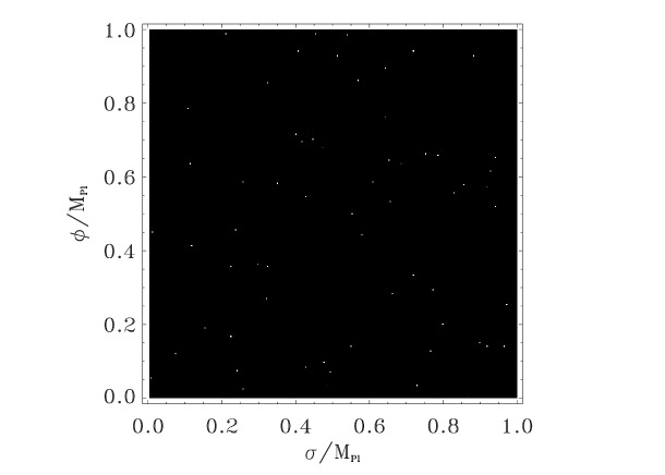
FIG. 1.: A plot of the space $(\phi_{\rm i},\sigma_{\rm i})$ of initial conditions for hybrid inflation. White regions correspond to initial conditions which give rise to successful inflation ($N_{\rm efold}\geq 70$), while black regions correspond to initial conditions which quickly lead the fields to the $\sigma_{\pm}$ minima with no successful inflation. Although hard to see, the successful region is a very narrow strip at the $\sigma=0$ axis, along with some scattered points off-axis. These plots were obtained with $\lambda=\lambda^{\prime}=1$, $m=5\times 10^{-6}M_{\rm Pl}$ and $M=2\times 10^{-2}M_{\rm Pl}$, which satisfies the COBE normalization.

We have carried out numerical simulations to ascertain which regions of initial condition space lead to successful inflation. Fig. 1 shows a plot of the space of initial conditions with the points which give rise to inflation shown in white. Here and in the other figures in this paper we used $\dot{\phi}=\dot{\sigma}=0$ which is the most favorable case; non-zero values for the derivatives of $\phi$ and $\sigma$ will make the fields roll faster along the potential. The portion of the space of initial conditions which gives rise to inflation is very small; apart from isolated points away from the $\sigma=0$ axis, the space of successful initial conditions is restricted to a rather hard to see strip along that axis, as suggested by Eq. (6). In other words, considerable fine tuning in the initial conditions is needed in order to get successful inflation. This result is in agreement with the results obtained in Ref. [7].

We note that the change in behaviour with varying initial conditions can be very sudden. In principle Fig. 1 has a grey scale showing the number of $e$-foldings if less than 70, with black corresponding to no inflation at all, but in practice the transition between sufficient inflation and no inflation is extremely swift. Another implication of this result concerns the extent to which the universe must be in a homogeneous state prior to inflation. If neighbouring regions have such vastly different evolution, this may suggest that even mild inhomogeneities will prevent inflation. However, such a general statement may not be true; the final outcome will depend on the dynamical effect of the gradients on the evolution of the scalar fields. This has been discussed, albeit in a different context, by Goldwirth and Piran [10], but more detailed investigation remains necessary.

III Possible resolutions

In this section, we study several mechanisms which may lessen the problem of finding viable initial conditions.

A Including other material

Since the problem is that inflation is unable to start, there is no rationale for considering a universe devoid of matter other than the scalar field. The inclusion of extra material provides an additional friction to the motion of the scalar field, which helps it towards the slow-roll regime. The natural assumption is that we are attempting to initiate inflation from within a radiation era, with the scalar field coming to dominate. Such radiation will certainly help ease the problem of initial conditions; the question is whether it does so significantly or not.

In this case the condition for the beginning of inflation mentioned in the previous section takes the form

$$\frac{\sigma}{M_{\rm Pl}}<\left(\frac{\lambda}{4}M^{4}+\rho_{\rm rad}\right)^{1/2}\frac{1}{\sqrt{\lambda^{\prime}}\,M_{\rm Pl}^{2}}\,.$$ (7)

If we note that the COBE normalization requires $M<3\times 10^{-3}M_{\rm Pl}$, then in order to have inflation even for large values of $\sigma$, we would need $\rho_{\rm rad}^{1/4}\sim M_{\rm Pl}$, which does not make much sense since we are supposed to be much below the Planck scale. Furthermore, since radiation redshifts as $a^{-4}$, any small effect which might be caused by the radiation fluid quickly becomes negligible.

Our numerical simulations confirm this simple estimate and show that the addition of a radiation fluid to our system does not significantly ease the onset of inflation.

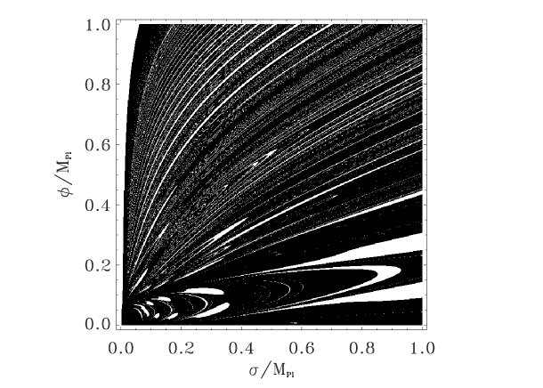
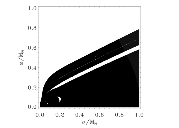
FIG. 2.: A plot of the space $(\phi_{\rm i},\sigma_{\rm i})$ of initial conditions for hybrid assisted inflation with $5$ copies (left panel) and $50$ copies (right panel) of the scalar field sector. We assumed copies of the original potential with the same masses and initial conditions. As before, the white regions indicate successful inflation, and the grey scale denotes the number of $e$-foldings with black corresponding to none.

B Extra scalar fields

One resolution to the problem of initial conditions which has been discussed is the possibility of an earlier period of inflation which sets the initial conditions for the hybrid inflation [15, 3]. This does not however appear to be a particularly natural evasion, because the question of whether suitable initial conditions exist for inflation is simply transported onto this new earlier inflation. However one way in which inflation may help is if there are many very similar, or even identical, scalar fields as in the case of assisted inflation [16]. Such a situation can arise with the compactification of a higher-dimensional scalar field, in which many four-dimensional scalar fields arise as the Kaluza–Klein tower of states [17].

Assuming we have $n$ copies of the potential, the Friedmann equation (2) is replaced by

$$H^{2}=\frac{1}{3M_{\rm Pl}^{2}}\sum_{i=1}^{n}\left[\frac{1}{2}\left(\dot{\phi_{i}}^{2}+\dot{\sigma_{i}}^{2}\right)+V(\phi_{i},\sigma_{i})\right]\,,$$ (8)

where all the copies of the inflaton and the second scalar field still obey Eq. (3).

Fig. 2 shows the results of our numerical simulations, where we assumed all the copies of the scalar fields had the same masses and initial conditions. With even a moderate number of copies of the potential, the onset of inflation is now possible in most of the space of permitted initial conditions. The situation improves the more copies of the fields there are. Further simulations we carried out show that provided at least one of the sets of fields starts in a region which would inflate in the model with only one set of fields, then inflation will be able to start. Even if none of the sets of fields is in a region which would give rise to inflation in the original model, inflation can still start in most cases.

It is interesting to note that the plots exhibit a fractal-like structure with new filaments appearing at every scale. Although we have not pursued this point, it is not surprising because it is known that two-field models of inflation can show chaotic behavior [18]. The hybrid inflation model can be seen as two coupled harmonic oscillators and it is well known that such systems usually exhibit chaotic behavior.

While successful in alleviating the initial conditions problem, the drawback is that we have simply presumed that it is possible to obtain large numbers of copies of the hybrid inflation sector. We are not aware of any mechanism which is capable of replicating the complicated hybrid inflation sector; the Kaluza–Klein implementation of assisted inflation [17] does not give such a simple outcome in the case of coupled fields.

C Brane cosmology

The realization [19] that we may live on a so-called ‘brane’ embedded in a higher-dimensional cosmology has enormous implications for cosmology. One such is the possibility of a modification to the Friedmann equation at high energies; Binétruy et al. [20] and, in a more general sense, Shiromizu et al. [21] have shown that the Friedmann equation can acquire a term proportional to the density squared (see also Ref. [22] for discussion of perturbations). This naturally provides additional friction operative at high energies.

We will consider here a five-dimensional model similar to the one used by Maartens et al. [23] in their study of chaotic inflation on the brane. In this case the Friedmann equation takes the form

$$H^{2}=\frac{\Lambda_{4}}{3}+\left(\frac{1}{3M_{\rm Pl}^{2}}\right)\rho+\left(\frac{4\pi}{3M_{5}^{3}}\right)^{2}\rho^{2}+\frac{{\cal E}}{a^{4}}$$ (9)

where $M_{5}$ is the fundamental five-dimensional Planck mass, which is taken as much smaller than $M_{\rm Pl}$. The effective cosmological constant on the brane, $\Lambda_{4}$, can be expressed in terms of the five-dimensional cosmological constant in the bulk, $\Lambda$, the tension of the brane $\lambda_{\rm b}$, and the fundamental scale $M_{5}$ as

$$\Lambda_{4}=\frac{4\pi}{M_{5}^{3}}\left(\Lambda+\frac{4\pi}{3M_{5}^{3}}\lambda_{b}^{2}\right)\,.$$ (10)

To have a negligible cosmological constant in the early universe requires $\Lambda=-4\pi\lambda_{b}^{2}/3M_{5}^{3}$. The effective four-dimensional Plank mass can be expressed in terms of $\lambda_{b}$ and $M_{5}$ as

$$M_{\rm Pl}=\sqrt{6}\,\left(\frac{M_{5}^{3}}{\sqrt{\lambda_{b}}}\right)\,.$$ (11)

As usual, in Eq. (9), $\rho=\dot{\phi}^{2}/2+\dot{\sigma}^{2}/2+V(\phi,\sigma)$.

The constant ${\cal E}$ in Eq. (9) describes the effect of massive gravitons on the brane and its origin can be traced to the projection of the five-dimensional Weyl tensor [21]. We will from now on neglect this term. It is clear that the presence of the $a^{4}$ denominator will suppress it during inflation. Although this term may not be negligible at the beginning of inflation, it will contribute to the friction term in the equations of motion for the scalar fields and can in principle also help alleviate the fine tuning in the initial conditions provided ${\cal E}$ is positive.

The equations of motion for the fields $\phi$ and $\sigma$ take the usual form, Eq. (3). Using Eqs. (10) and (11) in Eq. (9), and putting $\Lambda_{4}=0$ and ${\cal E}=0$ the Friedmann equation becomes

$$H^{2}=\frac{1}{3M_{{\rm Pl}}^{2}}\rho\left(1+\frac{\rho}{2\lambda_{b}}\right)\,.$$ (12)

From the previous equation we see that for high energies ($\rho>\lambda_{b}$) the quadratic term dominates; later on during the radiation epoch, this term will be redshifted by a factor $a^{-8}$ and should therefore become negligible. In order that no incompatibilities arise with nucleosynthesis the brane tension must satisfy $\lambda_{b}\gtrsim 1\,{\rm MeV}^{4}$, implying $M_{5}>10\,{\rm TeV}$ [24]. Here we will mainly be interested in the case where the quadratic term in $\rho$ dominates during inflation, that is $\lambda_{b}\ll V$.

As in the case of hybrid inflation in the standard four-dimensional context, the masses $m$ and $M$ cannot be freely chosen but are constrained by the COBE normalization of the spectrum of density perturbations. The calculation follows closely that of Ref. [1] for the standard four-dimensional case. In our model the slow-roll parameters are given by [23]

$$\epsilon\simeq 2M_{\rm Pl}^{2}\,\left(\frac{V^{\prime}}{V}\right)^{2}\frac{\lambda_{b}}{V}\quad;\quad\eta\simeq 2M_{\rm Pl}^{2}\,\left(\frac{V^{\prime\prime}}{V}\right)\frac{\lambda_{b}}{V}\,,$$ (13)

where we assumed $V\gg\lambda_{b}$. The spectrum of density perturbations takes the form [13]

$$\delta_{\rm H}^{2}\simeq\frac{1}{600\pi^{2}M_{\rm Pl}^{6}}\frac{V^{3}}{{V^{\prime}}^{2}}\frac{V^{3}}{\lambda_{b}^{3}}\,,$$ (14)

and the number of $e$-foldings is

$$N\simeq-\frac{1}{2M_{\rm Pl}^{2}}\int_{\phi_{i}}^{\phi_{f}}\frac{V^{2}}{\lambda_{b}V^{\prime}}d\phi\,.$$ (15)

Although there is no general analytical expression for the relation between the masses, there are two limits where an analytical expression for the masses can be found. When the quadratic term in the potential dominates we have chaotic inflation, which is essentially the same case as analyzed by Maartens et al. [23]. We are interested in the case where the false vacuum energy dominates, where we have

$$M=1.4\times 10^{-1}\left(\lambda\lambda^{\prime}\right)^{-1/6}\eta^{1/3}e^{20\eta}\lambda_{\rm b}^{1/6}M_{\rm Pl}^{1/3}\,\,,$$ (16)

where

$$\eta=\frac{3}{\pi^{2}}\frac{m^{2}M_{5}^{6}}{M^{8}}\,.$$ (17)

Using the slow-roll condition $\eta<1$, we can obtain an upper limit for the mass $m$:

$$m<6.2\times 10^{-5}\left(\frac{\lambda}{{\lambda^{\prime}}^{2}}\right)^{1/3}\eta^{4/3}e^{80\eta}\lambda_{\rm b}^{1/6}M_{\rm Pl}^{1/3}\,.$$ (18)

We are assuming $\lambda M^{4}/4\gg m^{2}\phi^{2}/2$, which imposes a further constraint

$$\eta^{3}e^{240\eta}\ll 2.3\times 10^{6}\,\frac{{\lambda^{\prime}}^{2}}{\lambda}\,,$$ (19)

which, for $\lambda=\lambda^{\prime}=1$, saturates for $\eta=\eta_{\rm MAX}=0.09$. This is exactly the same constraint as in the standard cosmological scenario (compare with Eq. (2.45) in Ref. [1]). Using this constraint in Eqs. (16) and (18), the vacuum domination approximation gives

$$\lambda^{1/4}M < 3.8\times 10^{-1}\left(\lambda\lambda^{\prime}\right)^{-1/6}\lambda_{\rm b}^{1/6}M_{\rm Pl}^{1/3}\,;$$ (20)

$$m < 1.1\times 10^{-3}\left(\frac{\lambda}{{\lambda^{\prime}}^{2}}\right)^{1/3}\lambda_{\rm b}^{1/6}M_{\rm Pl}^{1/3}\,\,.$$ (21)

When $\eta\ll 1/20$, the exponential in Eq. (16) can be neglected and we obtain a relation between $M$ and $m$;

$$M=0.8\left(\lambda^{5}\lambda^{\prime}\right)^{-1/22}\lambda_{\rm b}^{3/22}m^{2/11}M_{\rm Pl}^{3/11}$$ (22)

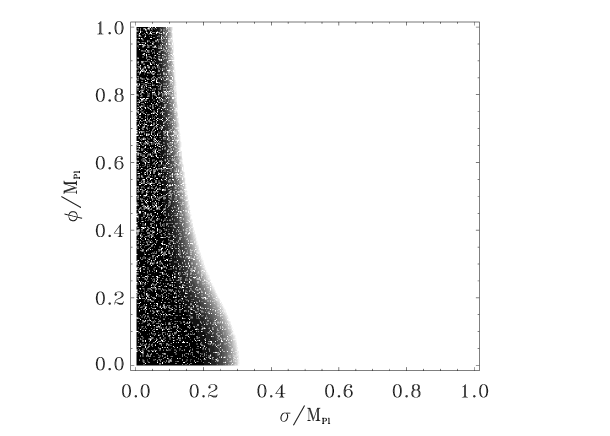
FIG. 3.: This plot shows the space of initial conditions for hybrid inflation on the brane, with $\lambda_{b}=6\times 10^{-8}\,M_{{\rm Pl}}^{4}$, $m=2\times 10^{-6}\,M_{{\rm Pl}}$, and $M=10^{-2}\,M_{{\rm Pl}}$. As before, white indicates regions of successful inflation.

Fig. 3 shows our results for hybrid inflation on the brane. The $\rho^{2}$ term is indeed efficient in broadening the region in the space of initial conditions where inflation occurs. As we decrease the value of $\lambda_{b}$, the onset of inflation becomes even easier as this further increases the friction term in the scalar field equations of motion. There is also a smoother transition between regions where successful inflation occurs (at least $70$ $e$-foldings of expansion) and those where inflation cannot start.

IV Conclusions

It is debatable whether one should be too concerned that only a limited region of initial condition space leads to sufficient hybrid inflation in the models we’ve considered, as one can readily argue, either probabilistically or anthropically, that the Universe we live in would originate from one of these regions. Nevertheless, it is a relevant question as to whether or not the problem is mitigated once the scenario is generalized beyond a universe containing only the scalar field, and we have studied several alternatives.

The assumption that filling the universe with some other material besides the scalar fields needed for hybrid inflation would help does not work as one might expect, mainly because a radiation fluid with a physically reasonable density will not decrease the friction timescale sufficiently to induce the onset of inflation. When we add a large number of copies of the potential to our original model, in the spirit of assisted inflation, we can in principle obtain inflation from most of the space of initial conditions. However, as we pointed out before it is not obvious how such a number of fields could be introduced in a physically sensible manner.

Finally, we have studied hybrid inflation in the context of brane cosmology. Using a simple model, we were able to show the hybrid inflation on the brane does not suffer from the same fine-tuning problems in the initial conditions as its standard counterpart. Since brane cosmology has become such a popular topic, it is encouraging to know that besides being a possible solution for the hierarchy problem, it is also possible to have inflation on the brane and, furthermore, free from some of the fine-tuning problems that plagued conventional inflation.

REFERENCES

- [1] E. J. Copeland, A. R. Liddle, D. H. Lyth, E. D. Stewart, and D. Wands, Phys. Rev. D 49, 6410 (1994); D. H. Lyth, hep-ph/9904371.
- [2] A. Linde and A. Riotto, Phys. Rev. D 56, 1841 (1997).
- [3] G. Lazarides and N. Tetradis, Phys. Rev. D 58, 123502 (1998).
- [4] Z. Berezhiani, D. Comelli, and N. Tetradis, Phys. Lett. 431B, 286 (1998).
- [5] D. H. Lyth and A. Riotto, Phys. Rept. 314, 1 (1999).
- [6] A. Linde, Phys. Lett B 259, 38 (1991); M. C. Bento, O. Bertolami and P. M. Sá, Phys. Lett. B 262, 11 (1991); A. Linde, Phys. Rev. D 49, 748 (1994).
- [7] N. Tetradis, Phys. Rev. D 57, 5997 (1998). (See also G. Lazarides and N. D. Vlachos, Phys. Rev. D 56, 4562 (1997) for an early analysis of the problem in the context of supersymmetric hybrid inflation).
- [8] T. Vachaspati and M. Trodden, Phys. Rev. D 61 023502 (2000).
- [9] E. Fahri and A. H. Guth, Phys. Lett. 183B, 149 (1987); J. Kung and R. Brandenberger, Phys. Rev. D 40, 2532 (1989); D. Goldwirth and T. Piran, Phys. Rev. Lett. 64, 2852 (1990).
- [10] D. Goldwirth and T. Piran, Phys. Rept. 214, 223 (1992).
- [11] A. D. Linde, Phys. Lett. B327, 208 (1994); A. Vilenkin, Phys. Rev. Lett. 72, 3137 (1994)
- [12] G. Felder, L. Kofman, and A. D. Linde, Phys. Rev. D 60 103505 (1999).
- [13] A. R. Liddle and D. H. Lyth, Phys. Rep. 231, 1 (1993); A. R. Liddle and D. H. Lyth, Cosmological inflation and large-scale structure, Cambridge University Press, Cambridge (2000).
- [14] E. F. Bunn and M. White, Astrophys. J. 480, 6 (1997).
- [15] C. Panagiotakopoulos and N. Tetradis, Phys. Rev. D 59, 083502 (1998).
- [16] A. R. Liddle, A. Mazumdar, and F. E. Schunck, Phys. Rev. D 58, 061301 (1998).
- [17] P. Kanti and K. A. Olive, Phys. Lett. 464B, 192 (1999).
- [18] N. J. Cornish and J. J. Levin, Phys. Rev. D 53, 3022 (1996); R. Easther and K. Maeda, Class. Quant. Grav. 16, 1637 (1999).
- [19] K. Akama, hep-th/0001113; V. A. Rubakov and M. E. Shaposhnikov, Phys. Lett B159, 22 (1985); N. Arkani-Hamed, S. Dimopoulos, and G. Dvali, Phys. Lett. 429B, 263 (1998); M. Gogberashvili, Europhys. lett. 49, 396 (2000); L. Randall and R. Sundrum, Phys. Rev. Lett. 83, 4690 (1999).
- [20] P. Binétruy, C. Deffayet, and D. Langlois, Nucl. Phys. B565 (2000) 269.
- [21] T. Shiromizu, K. Maeda, and M. Sasaki, gr-qc/9910076.
- [22] H. Kodama, A. Ishibashi, and O. Seto, hep-th/0004160; R. Maartens, hep-th/0004166; D. Langlois, hep-th/0005025; C. van de Bruck, M. Dorca, R. Brandenberger, and A. Lukas, hep-th/0005032.
- [23] R. Maartens, D. Wands, B. A. Bassett, and I. P. C. Heard, Phys. Rev. D 62, 041301 (2000).
- [24] J. M. Cline, C. Grojean, and G. Servant, Phys. Rev. Lett. 83, 4245 (1999).