The Rotation Curve of the Large Magellanic Cloud
and the Implications for Microlensing

Abstract

The rotation of the disk of the Large Magellanic Cloud (LMC) is derived from the radial velocities of 422 carbon stars (Kunkel, Irwin, & Demers 1997, A&AS, 122, 463). New aspects of this analysis include the propagation of uncertainties in the LMC proper motion with a Monte Carlo, and a self-consistent modeling of the rotation curve and disk kinematics. The LMC rotation curve reaches a maximum circular velocity of 72 $\pm$ 7 km s^-1 at $R=4.0$ kpc and then declines. The rotation curve is well fit by a truncated, finite-thickness exponential disk model with no dark halo, implying a total mass of 5.3 $\pm$ 1.0 $\times$ $10^{9}$ $M_{\odot}$. The velocity dispersion in concentric radial bins from $R=0.5$ to 5.6 kpc decreases from 22 to 15 km s^-1, then increases to $\sim$20 km s^-1 at larger radii. Constant-thickness disk models in virial equilibrium cannot be reconciled with the data even if the effects of LMC or Galactic dark halos are included. If the disk is virialized, the scale height rises from $h$ = 0.3 to 1.6 kpc over the range of $R$ = 0.5 to 5.6 kpc. Thus the LMC disk is flared. We model the velocity dispersion at large radii ($R>$ 6 kpc) as a maximal flared disk under the influence of the Galactic dark halo, which favors a mean density for the latter of $\overline{\rho}\sim 2.5\times 10^{-4}$ $M_{\odot}$ pc^-3 at the LMC distance.

LMC stellar kinematics play an important role in elucidating the nature of MACHOs, a dark population inferred from LMC microlensing. We have constructed a truncated and flared maximal disk model for the LMC which is kinematically based. Our model does not include a nonvirialized component such as tidal debris. The instantaneous probability of microlensing from LMC stars in our model is $\tau<1.0\times 10^{-8}\cdot{\rm sec}^{2}i$, where $i$ is the disk inclination. Our upper limit on the self-lensing optical depth is in good agreement with that obtained from less sophisticated models, and is an order of magnitude too small to account for the MACHO microlensing signal.

1 Introduction

If the Galactic dark halo were composed entirely of massive compact halo objects (MACHOs), the instantaneous probablity of microlensing (the “optical depth”) towards the Large Magellanic Cloud (LMC) would have been $\tau\sim 5\times 10^{-7}$ (Paczýnski 1986). The most recent observational result for MACHOs with masses up to about 1 $M_{\odot}$ is $\tau=1.2^{+0.4}_{-0.3}\times 10^{-7}$, which comes from an analysis of 5.7 years of LMC microlensing survey data (Alcock et al. 2000). Thus an all-MACHO Galactic dark halo is ruled out. However, the observed optical depth is significantly higher than the estimate for known Galactic and LMC stellar populations, $\tau\lower 2.15277pt\hbox{$\,\buildrel<\over{\sim}\,$}4\times 10^{-8}$ (Alcock et al. 2000). The excess LMC microlensing signal may be telling us the MACHO fraction of the Galactic dark halo or revealing gaps in our understanding of the essential structure of the LMC and Galaxy.

Critical discussions of the microlensing optical depth from known stellar populations have developed along two lines. One debate has been about the possible existence of a “new” stellar population which would account for the LMC microlensing result. Some example suggestions include an intervening dwarf galaxy or tidal stream (Zhao 1998; Zaritsky & Lin 1997, Zaritsky et al. 1999), and a very warped Galactic disk (Evans et al. 1998). These hypotheses have been tested, and in some cases ruled out (Alcock et al. 1997; Beaulieu & Sackett 1998; Bennett 1998; Gould 1998, 1999; Gyuk, Flynn, & Evans 1999; Ibata, Germaint, & Beaulieu 1999; Johnston 1998). The second debate has been about the importance of LMC star-star “self-lensing” (Sahu 1994; Wu 1994). In particular, although the LMC is well represented by an exponential disk model which often serves as the basis for the self-lensing optical depth calculation, it may exhibit some important detailed structures. Our paper is motivated by this LMC self-lensing problem.

The line-of-sight velocity dispersion of LMC stars yields a strong constraint on star-star self-lensing from the virialized LMC disk: $\tau\lower 2.15277pt\hbox{$\,\buildrel<\over{\sim}\,$}1\times 10^{-8}$ (Gould 1995). Gould’s elegant limit is probably uncertain by no more than a factor of $\sim$2. However, several LMC models have been devised which would increase the self-lensing optical depth over the Gould limit. One example of a detailed structure that might increase the self-lensing optical depth is a highly-inclined and flared LMC disk (Zhao 1999). It has also been suggested that the oldest LMC disk stars have a very large characteristic scale height, or that the LMC harbors an as yet unseen but massive stellar spheroid (e.g. Aubourg et al. 1999; Salati et al. 1999; Evans & Kerins 2000). Finally, it is possible that a nonvirialized stellar component (i.e., a shroud of tidal debris; Weinberg 2000) acts to increase the self-lensing optical depth (Zhao 1998).

Kinematic studies play a critical role in testing these various proposed LMC models. For example, the flare of the LMC disk may be inferred from its velocity dispersion at different radii, and the existence of a non-equilibrium stellar component lying near the LMC might be proven with a large kinematic survey (Zhao 1999; Graff et al. 1999; see also Zaritsky et al. 1999; Ibata et al. 1999). In addition, one could search directly for an LMC stellar population with a velocity dispersion of $\sim$50 km s^-1, the prediction for a spheroid or very thick disk. These latter components must be identified before their importance to the self-lensing optical depth can be assessed. The LMC rotation curve provides a framework for detailed kinematic studies such as these.

The decomposition of the LMC rotation curve into disk and dark halo components has several implications for microlensing. First, as emphasized by Gyuk et al. (1999), the total mass of the LMC is an important constraint on self-lensing optical depth calculations. A high-mass model will typically predict a high self-lensing optical depth, with an additional dependence on whether the mass lies mostly in the disk or in a halo. Unfortunately, recent analyses of the LMC rotation curve have lead to mass estimates that range over a factor of $\sim$4, which can be attributed primarily to different assumptions about a dark halo (Kim et al. 1998, Kunkel et al. 1997, Schommer et al. 1992). Second, a massive LMC dark halo might significantly affect the LMC disk kinematics (e.g. Bahcall 1984), with possible consequence for constraints on self-lensing or determining the flare of the disk. The influence of an LMC dark halo on the LMC disk kinematics has not been investigated in detail. We note that the interplay between the disk and dark halo is also of general interest for studies of galaxy formation and evolution. Finally, if the LMC has a dark halo with a physical makeup similar to that of the Galactic dark halo (i.e. composed partly of MACHOs), the MACHO fraction of the Galactic dark halo implied by the observed optical depth would be lowered (Alcock et al. 2000).

Motivated by the above considerations, we present a new analysis of the LMC rotation curve. In this work we are particularly concerned with the flare of the LMC disk. However, other issues pertinent to microlensing are discussed as our calculations and analyses permit. We refer extensively to the H I rotation curve recently presented by Kim et al. (1998) and the impressive radial velocity dataset for LMC carbon stars summarized by Kunkel, Demers, Irwin & Albert (1997; hereafter KDIA). A significant subset of these latter data are public (Kunkel, Irwin & Demers 1997), and archived electronically at the CDS. We also refer extensively to the analysis of the LMC space motion presented by Kroupa & Bastian (1997).

Our paper is organized as follows. In §2, we present the impetus for this work, a comparison of constant-thickness exponential disk models (with no dark halos) to the LMC disk velocity dispersions reported by KDIA. In §3, we reanalyze the LMC rotation curve and velocity dispersion curve using archived carbon-star radial-velocity data. In §4, we present a multi-mass component kinematic model for the LMC. In §5, we compare our carbon-star rotating disk solution to our model. We discuss the microlensing implications of our analyses in §6 and conclude in §7.

2 A Flared LMC Disk?

2.1 Theoretical Models for Disk Galaxies

Disks in galaxies often have exponential surface brightness profiles from which we infer exponential mass surface density profiles of the form

$$\Sigma(R)=\Sigma_{0}\ e^{-R/\Lambda}$$ (1)

by assuming constant mass-to-light ratios ($M/L$). In equation (1), $\Sigma_{0}$ is the central mass surface density, $\Lambda$ is the radial scale length, and $R$ is a cylindrical radial coordinate. For an infinitely thin disk described by equation (1), Freeman (1970) calculated that the rotation curve reaches a maximum circular velocity at $R\sim 2.2\Lambda$

$$V_{max}=0.623\ \left(\ \frac{G\ M_{disk}}{\Lambda}\ \right)^{1/2}$$ (2)

where $M_{disk}$ is the total mass of the disk, which is related to the central surface density by

$$M_{disk}\ =\ 2\pi\Sigma_{0}\Lambda^{2}$$ (3)

For the case of a disk with a modest finite thickness, $V_{max}$ will be decreased by $\sim 5\%$ (van der Kruit & Searle 1982). A useful model with a finite thickness is the exponential disk (also known as a double-exponential disk), which has a density distribution

$$\rho(R,z)=\rho_{0}\ e^{-|z|/h}\ e^{-R/\Lambda}$$ (4)

In equation (4), the variable $h$ is the vertical, or what we will sometimes refer to as the “z” scale height. If we choose the spatial density normalization $\rho_{0}=\Sigma_{0}/2h$, the exponential disk projects to the surface density of the infinitely thin Freeman disk, i.e. equation (1). The z-velocity dispersion, $\sigma_{z}$, for the exponential disk is given by Wainscoat, Freeman and Hyland (1989),

$$\sigma_{z}(R,z)=2h\ \left[\pi G\ \rho_{0}\ e^{-R/\Lambda}\left(1-\frac{1}{2}e^{-|z|/h}\ \right)\ \right]^{1/2}$$ (5)

which assumes that the disk is virialized. Equation (5) is strictly valid for a radially infinite disk. The radial dependence (i.e., the $e^{-R/\Lambda}$ term) in equation (5) scales the local density normalization, as prescribed by others (van der Kruit & Searle 1982; van der Kruit & Freeman 1984).

A model extensively discussed by van der Kruit & Searle (1981, 1981b, 1982) is the isothermal disk. The vertical distribution of stars in an isothermal disk is described by the sech² function, as originally derived by Spitzer (1942; see also §4.2 of this paper). The spatial density for this disk model is,

$$\rho(R,z)=\rho_{0}\ {\rm sech}^{2}(z/h)\ e^{-R/\Lambda}$$ (6)

which projects to the surface density of the infinitely thin Freeman disk if $\rho_{0}=\Sigma_{0}/2h$. Assuming virialization, the z-velocity dispersion of the isothermal disk is proportional to the z-scale height and independent of z:

$$\sigma_{z}(R)=h\ \left[2\pi G\ \rho_{0}\ e^{-R/\Lambda}\ \right]^{1/2}$$ (7)

where the radial dependence scales the local density normalization. Equation (7) is strictly valid for a radially infinite disk. We note that the “z-scale height” in the isothermal disk is not strictly a scale height (and not the same as $h$ in the double-exponential model), but it is a similar parameter. Further comparisons of the exponential and isothermal disk models are found in Wainscoat, Freeman & Hyland (1989), and van der Kruit (1988).

The systematic error in the velocity dispersion predicted by the radially infinite isothermal disk model has been shown to be only $\sim$10% in the range $1<R/\Lambda<4$ using numerical studies of truncated isothermal disk models (van der Kruit & Searle 1982). We will use the isothermal disk model in our analyses, because these numerical calculations provide us with an estimate of the model accuracy, and will later allow us to approximately account for the finite radial extent of the LMC disk (see §4.3 of this paper). Observations of edge-on spirals indicate that both the exponential and isothermal models are viable representations of real disks (de Grijs, Peletier, & van der Kruit 1997). The specific choice of model does not affect the main results of this work.

It is reasonable to compare the model z-velocity dispersion to the observed velocity dispersion at different projected radii in the LMC for the case of uniform anisotropy ($\sigma_{Z}/\sigma_{R}$ constant at different radii; van der Kruit & Freeman 1984). Although we do not know if this is true for the LMC, the assumption of uniform anisotropy is supported by kinematic studies of the old Galactic disk (Lewis & Freeman 1989). Gould (1995) notes that if $\sigma_{Z}/\sigma_{R}<$ 1 as found elsewhere, the line of sight velocity dispersion measured for an inclined disk overestimates $\sigma_{Z}$. Therefore, our model z-velocity dispersion is likely an upper-limit on the true z-velocity dispersion.

Combining equations (2), (3) and (7) yields

$$\sigma^{2}_{z}(R)\ \approx\ 1.288\ \left(\frac{h}{\Lambda}\right)\ V^{2}_{max}\ e^{-R/\Lambda}$$ (8)

which is most accurate for disks in the range $1<R/\Lambda<4$. The z-scale height has been observed to be constant over a large range of $R$ in numerous disk galaxies (van der Kruit & Freeman 1984; de Grijs, Peletier, & van der Kruit 1997), implying that $\sigma$ decreases with increasing $R$ in these galaxies. Indeed, this trend of decreasing velocity dispersion has been observed in over a dozen spiral/disk galaxies (Bottema 1993), including our own.

In summary, if the disk velocity dispersions are the same at different radii, the disk is likely flared (e.g. Zhao 1999). However, this inference assumes that (1) the disk is virialized, (2) the radial scale length is constant, (3) the disk velocity dispersions exhibit uniform anisotropy, and (4) the galaxy has no dark halo (or that the dark halo has a negligible affect on the disk velocity dispersions). Finally, one must be careful to compare the observed velocity dispersions to the simple model described above over a restricted range of radii, because real galactic disks are finite in radial extent. We compare to the LMC in the next section.

2.2 Comparison of Disk Models to the LMC

In this section, we will adopt a plausible value for the product $hV_{max}^{2}$ in equation (8), and compare that model to LMC disk velocity dispersion data. Following KDIA and many others, we adopt a distance to the LMC of 50.1 kpc, and an inclination of $i$ = 33 degrees. For comparison, wide-field UV polarimetric image data have yielded a precise but model-dependent estimate of the inclination of the LMC disk: $i=36^{+2}_{-5}$ degrees (Cole, Wood, & Nordsieck 1999). Westerlund (1997) summarizes a number of other inclination measurements.

We adopt $\Lambda=1.6$ kpc for the radial scale length of the LMC disk. The surface brightness profile of the LMC disk is well-fit by an exponential with a scale length $\Lambda\approx 1.6$ kpc (de Vaucouleurs 1957, Bothun & Thompson 1988). Moreover, the surface density profile of intermediate-age long period variables (LPVs) in the LMC is also fit by an exponential with a scale length of $\Lambda\sim 1.6$ kpc (Hughes, Wood & Reid 1991). This result directly associates our kinematic dataset with an LMC population that follows the $\Lambda$ = 1.6 kpc exponential profile, because some of the intermediate-age LPVs are also carbon stars. Finally, the RR Lyrae stars in the LMC also appear to lie in a $\Lambda\approx 1.6$ kpc exponential disk (Alcock et al. 2000b). Since the RR Lyraes are presumably much older than the carbon stars, the carbon stars were likely born into the same disk. We note that no stellar population in the LMC has yet been shown to be inconsistent with a $\Lambda=1.6$ kpc exponential profile. We assume that the carbon stars observed by KDIA properly represent this LMC disk.

The KDIA dataset consists of radial velocity measurements for 759 carbon stars spanning a true LMC radius of 2 to 10 kpc. KDIA summarize the results of 11 different zonal solutions for a rotating disk. In Figure 1, we plot the KDIA velocity dispersions as a function of radial distance, which we take as the central value for each zonal solution given in KDIA’s Table 1. We show data only for $R$ = 3 to 6 kpc. This is the range of radii where equation (8) will most accurately predict the velocity dispersions. The dashed line in Figure 1 is the mean of the plotted, observed velocity dispersions, $\sigma=$ 13.7 km s^-1. Assuming a constant value of $\sigma$ equal to the mean, we find $\tilde{\chi}^{2}$ = 0.4, consistent with the data. The solid line plotted in Figure 1 shows the prediction of equation (8) assuming values of $V_{max}=70$ km s^-1 and $h$ = 0.35 kpc at $R~{}=~{}2\times\Lambda$. This model predicts $\sigma_{z}~{}\approx~{}13.7$ km s^-1 at $R~{}=~{}2\times\Lambda\approx~{}3.2$ kpc. The fit for this model distribution is $\tilde{\chi}^{2}$ = 8.7, which can be rejected with high significance. Models with larger scale heights intersecting the data at larger $R$ give similarly poor fits. One possible interpretation of the observed constancy of $\sigma$ with $R$ is that the z-scale height increases as $\sim e^{+R/2\Lambda}$, i.e. the LMC disk is flared.

3 The LMC Rotation Curve Revisited

An alternate interpretation of Figure 1 might be a constant-thickness disk under the dynamical influence of a dark halo (Bahcall 1984). Indeed, Kim et al. (1998) compared their H I rotation curve with the KDIA carbon star rotation curve and, on this basis, argued that an LMC dark halo is dynamically significant at a radius of $\sim$4 kpc. However, KDIA favored a different interpretation; they attributed the rising outer portion of their carbon star rotation curve to tidal effects, and not a dark halo. Before concluding that the LMC disk is flared, it is worth testing disk plus dark halo kinematic models in a self-consistent manner. With this model comparison in mind, let us consider the KDIA analysis in greater detail.

We have several specific concerns with the KDIA analysis. First, and perhaps most importantly, KDIA excluded some carbon stars from their solutions for their association with a polar ring. This procedure might have artificially lowered the disk velocity dispersions. By retaining these stars in our solutions, we guarantee that our results will be properly comparable to our model (which will not include a polar ring). KDIA also corrected for the LMC transverse motion by forcing the position angle of the kinematic line of nodes to match the photometric line of nodes in each zonal solution. This is a questionable procedure. Moreover, it is inconsistent with the H I analysis by Kim et al. (1998). We will correct the carbon-star velocities for the transverse motion of the LMC in a manner consistent with the H I rotation curve analysis by Kim et al. (1998). In fact, we will make our carbon star rotation curve analysis similar in other ways to the H I rotation curve analysis (i.e., by adopting the same kinematic center), in order to lend maximum credibility to detailed comparisons of the two rotation curves.

3.1 Rotation Curve Solution

3.1.1 The Carbon Star Radial Velocity Data

We assemble positions (right ascension and declination; equinox 1950) and galactocentric radial velocities for Magellanic Cloud carbon stars from Kunkel, Irwin & Demers (1997). We discard all Small Magellanic Cloud (SMC) carbon stars, “inter-cloud” carbon stars (their Table 15), and carbon stars located near the center of the LMC (their Table 17; see also §3.3). We also discard one rogue carbon star (C0433$-$6607) for its highly discrepant velocity. The resulting homogeneous dataset contains 422 carbon stars, representing a significant subset of the data analyzed in KDIA. Ongoing observational campaigns to obtain carbon star radial velocities will likely increase the sample size in the coming years (Suntzeff 1998). The archival dataset we have assembled is sufficient for the purposes of this study.

3.1.2 Transverse Motion Radial Velocity Correction

Feast, Thackeray & Wesselink (1961) have discussed the apparent rotation induced by the transverse motion of the LMC. Each of our 422 carbon star velocities are corrected for this projected radial velocity gradient as follows. We adopt the LMC space motion calculated by Kroupa & Bastian (1997), which is derived from an average of the LMC proper motion they measure with Hipparcos data and the LMC proper motion measured by Jones, Klemola, & Lin  (1994). The Hipparcos and Jones et al. (1994) measurements of the LMC proper motion agree within their respective error bars. We note that Kim et al. (1998) make their transverse motion correction using the proper motion measurement by Jones et al. (1994).

It is useful to establish a Galactic coordinate system for the vector analysis that follows. Following Kroupa & Bastian (1997), the galactocentric coordinates used here are such that the Galactic Center and the Sun are located at 0 and $-8.5$ kpc along the $x$-axis, respectively. The positive $z$-axis points toward the north Galactic pole, and the positive $y$-axis points in the direction of Galactic rotation at the position of the Sun. In these coordinates, the position vectors of the Sun and LMC are

$$R_{\odot}\ =\ \left(-8.5,\ 0.0,\ 0.0\right)$$ (9)

$$R_{LMC}\ =\ \left(-1.0,\ -40.5,\ -26.6\right)$$ (10)

in units of kpc. The velocity vector of the LMC is

$$V_{LMC}\ =\ \left(+41\pm 44,\ \ -200\pm 31,\ \ +169\pm 37\right)$$ (11)

in units of km s^-1 (Kroupa & Bastian 1997). The galactocentric radial velocity of the LMC is the vector dot product $V_{LMC}~{}^{.}~{}\hat{R}_{LMC}=(41,-200,-169)~{}^{.}~{}(-1.0,-40.5,-26.6)/48.5=74$ km s^-1, where $\hat{R}_{LMC}$ is a normalized unit vector. The vector between the Sun and LMC is $X=R_{LMC}-R_{\odot}=(7.5,-40.5,-26.6)$, and the radial velocity component of the LMC seen from the local standard of rest (accounting for the Sun’s peculiar velocity and Galactic rotation) at the position of the Sun is $V_{LMC}~{}^{.}~{}\hat{X}_{LMC}=80$ km s^-1. The vector $X_{LMC}$ points toward the “center” of the LMC, which is assumed to be at $\ell=280.46$, $b=-32.89$ (Kroupa & Bastian 1997). The unit vector connecting the Sun to any position in the sky in galactocentric coordinates is

$$\hat{X}(b,\ell)\ =\ \left(\cos~{}b\cos~{}\ell,\ \ \cos~{}b\sin~{}\ell,\ \ \sin~{}b\right)$$ (12)

The transverse motion velocity correction that we seek is the difference between the projected radial velocity toward the LMC center and the projected radial velocity toward each carbon star. If we define the vector $\hat{S}=\hat{X}_{LMC}-\hat{X}(b,\ell)$, the apparent rotation induced by the LMC space motion is $\delta V(\ell,b)=\hat{S}~{}^{.}~{}V_{LMC}$. We make our correction by subtracting $\delta V(\ell,b)$ from the observed carbon star velocities. Small differences between the Kroupa & Bastian (1997) model used here for the transverse motion radial velocity correction and assumptions (i.e., for the LMC center and distance) in subsequent sections have a negligible effect on our results.

3.1.3 Zonal Solutions

First, we convert each carbon star’s right ascension and declination into spherical coordinates in units of radians. We designate these $\alpha$ and $\delta$, respectively. We adopt the center of the LMC at right ascension $05^{h}\ 17^{m}.6$ and declination $-69^{0}\ 02^{{}^{\prime}}.0$ (equinox 2000) following Kim et al. (1998). We designate the LMC center with $\alpha_{0}$ and $\delta_{0}$ (also in units of radians and precessed to equinox 1950). The distribution of carbon stars is shown in Figure 2 (where North is up and East is to the right). The SMC is located well outside of the boundaries of the figure in a South-Westerly direction (toward the lower left). We remind that $\alpha$ and $\delta$ are spherical coordinates plotted on a rectilinear scale. Therefore, the distribution of carbon stars shows a $\sim$cos($\delta$) distortion.

Our solution proceeds as follows. We calculate the position angle ($\Theta$) and radial distance from the center of the LMC ($S$ in units of radians) for each carbon star using the formulae

$$S=\cos^{-1}\left[\ \sin\delta_{0}\ \sin\delta\ +\ \cos\delta_{0}\ \cos\delta\ \cos(\alpha-\alpha_{0})\ \right]$$ (13)

$$\Theta^{\prime}=\sin^{-1}\left[\frac{\cos\delta_{0}\ \sin(\alpha-\alpha_{0})}{\sin S}\right]$$ (14)

$$\Theta=2\pi-\Theta^{\prime}_{NE},\ \Theta=\pi+\Theta^{\prime}_{SE},\ \Theta=-\Theta^{\prime}_{NW},\ \Theta=\pi+\Theta^{\prime}_{SW}\$$ (15)

Equation (15) assigns the correct sign and phase to the position angle depending on which quadrant each star resides in Figure 2. We have defined $\Theta$ to increase West of North. We deproject each radial distance on the sky to true LMC radius ($R$ in units of kpc) using,

$$R=50.1\ \left|\tan^{-1}\left(\ S\ \cos(\Theta+\Theta_{0})\ \left[1\ +\ \tan^{2}(\Theta+\Theta_{0})\sec^{2}i\right]^{1/2}\ \right)\right|$$ (16)

We take the absolute value of the inverse tangent in equation (16) to guarantee a positive value for $R$. We accommodate a twisting disk model by introducing $\Theta_{0}$. The parameter $\Theta_{0}$ allows for a changing kinematic line of nodes in different radial zone solutions. We note that $\Theta_{0}$ is sensitive to the adopted LMC transverse velocity (Meatheringham et al. 1989). We define our different zones by making cuts in true radius. Each zonal solution is derived by fitting the function $V(\Theta)$ to the distribution of galactocentric radial velocities,

$$V(\Theta)\ =\pm\left(\ \frac{V_{c}\ \sin i}{\left[\ 1\ +\ \tan^{2}(\Theta+\Theta_{0})\sec^{2}i\ \right]^{1/2}}\ +\ V_{sys}\right)$$ (17)

We must choose the correct sign for $V(\Theta)$ at the appropriate position angle, which is the meaning of the ‘$\pm$’ in equation (17). We choose ‘$+$’ for $(\Theta+\Theta_{0})$ = $-\pi/2$ to $\pi/2$, and ‘$-$’ for $(\Theta+\Theta_{0})$ = $\pi/2$ to $3\pi/2$. The fitted model could be generalized to account for a warped and decentered disk by letting $i$ and ($\alpha_{0}$, $\delta_{0}$) vary in each zonal solution. However, we fix $i$, $\alpha_{0}$, and $\delta_{0}$ to the values given above in all solutions.

We derive solutions in four radial zones which span $R$ = 2.5 - 5, 5 - 6, 6 - 7, and 7 - 13 kpc. These were chosen to provide an adequate number of stars and phase coverage in each zone. The inner-most and outer-most boundaries were chosen to be inclusive of the entire dataset when $\Theta_{0}$ = 0. We begin by solving for $V_{sys}$, $\Theta_{0}$, and $V_{c}$ that yield a minimum dispersion about $V(\Theta)$ in each of our zones. We average the values of $V_{sys}$, excluding the outermost zone (which was sometimes poorly constrained). In a second round of fitting, we fix $V_{sys}$ to the three-zone average value, and search only for values of $\Theta_{0}$ and $V_{c}$ that minimize the velocity dispersion. This procedure was easily reproduced, and facilitated our bootstrap and Monte Carlo error analyses (described below).

The mean radii in each final zonal solution are $<R>$ = 4.0, 5.6, 6.5, and 7.8 kpc. The minimum velocity dispersions occurred at $\Theta_{0}$ = $-$37, $-$22, $-$8, and 3 degrees . We find circular velocities $V_{c}$ = 72, 68, 65, and 65 km s^-1 and velocity dispersions $\sigma$ = 17.7, 14.9, 19.3 and 20.6 km s^-1, respectively (in order of increasing radius). The four zonal solutions are shown in Figure 3. We indicate the carbon stars with small open circles. Each carbon star is plotted twice at $\Theta$ and ($\Theta$ + $2\pi$). The best fit curve is plotted as a solid line. The mean radius, circular velocity, and velocity dispersion are also labeled in each panel.

3.2 Rotation Curve Error Analysis

Our first estimate of the errors is made with a bootstrap resampling analysis (Barrow, Sonada, & Bhavsar 1984). We create 250 artificial datasets by randomly removing 1-10% of the carbon stars from our full dataset, and then find new rotating disk solutions for each of these. In a bootstrap reasampling analysis, the variances in the mean values of interest averaged over all of the artificial datasets are taken to represent the internal variances of the full dataset. We find errors in $V_{c}$ of 1.3, 1.7, 2.3, and 2.4 km s^-1 for the four radial zones (in order of increasing radii). We find an error in $\sigma$ of 0.3, 0.2, 0.4, and 0.5 km s^-1, and errors in $\Theta_{0}$ of 1.1, 1.0, 2.4, and 1.5 degrees, respectively.

Our second calculation is designed to estimate the errors associated with our choice of zonal boundaries and the movement of stars between zones due to the changing $\Theta_{0}$ parameters. For each of the four zones, we find new solutions for 64 different variations in the zonal boundaries. We varied each boundary by no more than $\pm$ 0.25 kpc, which yielded roughly comparable numbers of stars and mean radii in each zonal solution (except for the outer boundary of the outer-most zone which was varied by 1.5 kpc in steps of 0.25 kpc). The variances of $V_{c}$, $\sigma$, and $\Theta_{0}$ in the zonal boundary solutions are similar to those found with the bootstrap analysis. Moreover, we find no systematic trends with boundary choice, except for the outermost zone. In the outermost zone, $V_{c}$ decreases systematically (from $\sim$60 to 30 km s^-1) as the inner boundary is varied from $\sim$6.7 to 7.2 kpc.

Finally, we perform a Monte Carlo calculation to propagate the error on the LMC space motion to the rotation curve. We create 500 artificial datasets, where the LMC space motions are drawn randomly from a sample that reproduces the best fit values and errors in equation (11). We assume Gaussian distributions for the space motion errors. This calculation yields errors in $V_{c}$ of 7.1, 8.7, 10.4 and 15.8 km s^-1, errors in $\sigma$ of 0.1, 0.2, 0.3 and 0.4 km s^-1, and errors in $\Theta_{0}$ of 6.6, 4.6, 7.6 and 8.4 degrees, in the four zones (in order of increasing radius). Similar values were found with as few as $\sim$250 artificial datasets, indicating that our calculation is robust. For most of the parameters in our rotating disk solution, the error from the LMC space motion dominates. Our final solutions and adopted errors are summarized in Table 1.

We note that there would be no stars in common between the different solutions if all zones had the same $\Theta_{0}$, but in our final solutions, $\sim$5% of the stars are located in two zones (see Table 1). However, since we have accounted for the movement of small numbers of stars across the zonal boundaries in our error analysis, we may consider each zonal solution as independent in subsequent analyses.

3.3 Velocity Dispersion in the LMC Bar

We previously discarded 22 radial velocity measurements for carbon stars very near the center of the LMC (Kunkel, Irwin & Demers 1997; their Table 17) because this sample of stars did not span an adequate range of $\Theta$ to yield an interesting zonal rotation curve solution. However, the velocity dispersion of these carbon stars is of considerable interest. This sample of stars at $<R>=0.5$ kpc has a velocity dispersion of $\sigma=22.1$ km s^-1. Guided by our error analyses above, we adopt an error of 1 km s^-1. The average velocity dispersion of carbon stars in our five zones is $\sigma$ = 18.9 km s^-1. We defer further discussion and interpretation of the LMC rotation curve and disk velocity dispersions until §5, after we present our theoretical kinematic model.

4 A Multi-Mass Component Model for the LMC

4.1 Rotation Curve

We will consider two representations of the contribution of the luminous mass in the LMC disk to the rotation curve. The first is derived empirically by Kim et al. (1998) from the $R$-band surface brightness data of de Vaucouleurs (1958). For two assumptions of the disk mass-to-light ratio, we present this stellar rotation curve in Table 2. The second representation of the disk rotation curve we will consider is the finite-thickness, truncated disk model of van der Kruit and Searle (1982). We adopt their model No. 2 (truncated at $R$ = 4$\Lambda$) from their Appendix A.1. Table 3 summarizes this disk model rotation curve, which is given in units of the radial scale length ($\Lambda$) and the equivalent maximum circular velocity for an infinitely thin exponential disk ($V_{max}$; see §2.1 of this paper). This model will also be used to calculate a correction to the scale heights inferred from the disk velocity dispersions at small radii in the LMC (see §4.3 of this paper).

When comparing either of these two disk rotation curves to our carbon star data points, we will add in quadrature the small additional contribution of gas in the LMC disk to the rotational velocity. Kim et al. (1998) calculated the gas rotation curve using the single-dish H I data of Luks & Rolfs (1992), and assuming a 30% contribution from He I. The gas rotation curve is summarized in Table 4.

Finally, we will account for a pseudo-isothermal dark halo in the traditional manner, assuming a density profile,

$$\rho_{halo}(R)\ =\ \frac{\rho_{0}}{1\ +\ \left(R^{2}/a^{2}\right)}$$ (18)

where the circular velocity is a function of the integrated total mass

$$V^{2}_{halo}(R)\ =\ 4\pi G\rho_{0}a^{2}\left[1\ -\ \frac{a}{R}\tan^{-1}\left(\frac{R}{a}\right)\ \right]$$ (19)

The psuedo-isothermal dark halo is parameterized by a central density, $\rho_{0}$, and core radius, $a$. We add the circular velocities of the disk ($V_{disk}$) and psuedo-isothermal halo ($V_{halo}$) in quadrature in order to calculate the rotation curve of our model: $V_{c}(R)$.

4.2 Disk Velocity Dispersions

The effect of a spherical dark halo on the velocity dispersion of an embedded disk has been extensively discussed by Bahcall (1984), Bahcall & Casertano (1984) and Bottema (1993). The vertical motions of stars in a disk and halo system are governed by Poisson’s equation

$$\frac{\partial^{2}\phi}{\partial z^{2}}\ =\ 4\pi G\left(\rho_{disk}\ +\ \rho^{eff}_{halo}\right)$$ (20)

where

$$\rho^{eff}_{halo}\ =\ \rho_{halo}\ -\ \frac{1}{4\pi GR}\ \frac{\partial}{\partial R}\ V^{2}_{c}(R)$$ (21)

and the first moment of the Boltzmann equation

$$<\sigma^{2}_{z}>\ \frac{\partial\rho(z)}{\partial z}\ =\ -\frac{\partial\phi}{\partial z}\ \rho(z)$$ (22)

The effective halo density, $\rho^{eff}_{halo}$, includes the contribution from the radial deriviative of the total circular velocity, $V_{c}$. If the rotation curve is fairly flat, we may discard the radial deriviative term in equation (22) and equate $\rho^{eff}_{halo}=\rho_{halo}$. This formulation of the problem (Bahcall 1984) neglects the $<\sigma_{z}\sigma_{R}>$ cross terms in Poisson’s equation. With the following redefinitions (Bahcall 1984)

$$z_{0}=\left(\frac{<\sigma^{2}_{z}>}{2\pi G\rho_{disk}(z=0)}\right)^{1/2},\ \ \ x=\frac{z}{z_{0}}\ \ ,\ \ \ y(x)=\frac{\rho_{disk}(x)}{\rho_{disk}(x=0)}$$ (23)

and

$$\epsilon=\frac{\rho^{eff}_{halo}(z=0)}{\rho_{disk}(z=0)}$$ (24)

we rewrite the equations governing the vertical motions of the disk stars as

$$y\frac{d^{2}y}{dx^{2}}\ -\ \left(\frac{dy}{dx}\right)^{2}\ =\ -2y^{2}\ -\ 2\epsilon y^{2}$$ (25)

with the boundary conditions

$$y(0)\ =\ 1\ ,\ \ \ \left(\frac{dy}{dx}\right)_{x=0}\ =0$$ (26)

The solution for $\epsilon$ = 0 was first published by Spitzer (1942):

$$y\ =\ {\rm sech}^{2}x$$ (27)

The solution to equation (25) for $\epsilon>>1$ is

$$y\ =\ e^{-\epsilon x^{2}}$$ (28)

The differential equation (25) must be solved numerically for intermediate values of $\epsilon$.

The $\epsilon$ parameter define in equation (24) is the ratio of effective halo density to the disk density in the plane of the disk. It is particularly useful parameter because it relates ratio of the velocity dispersion in a disk plus halo system, $\sigma_{disk+halo}$, to the velocity dispersion in a disk with no halo, $\sigma_{disk}$. Following Bottema (1993), and suppressing the subscript $z$ for clarity,

$$\frac{\sigma_{disk+halo}}{\sigma_{disk}}\ =\ \alpha^{-1}$$ (29)

where $\alpha$ is the surface density

$$\alpha=\int\limits^{\infty}\limits_{0}y(x)dx$$ (30)

In the limit of $\epsilon>>1$,

$$\alpha^{-1}=\ 2\left(\frac{\epsilon}{\pi}\right)^{1/2}$$ (31)

We have solved for $\alpha^{-1}$ as a function of $\epsilon$ numerically; these values are listed in Table 5. In the limit of large $\epsilon$, these values confirm equation (31). The error in $\alpha$ is $\sim$30% at $\epsilon\sim 1$ and less than 20% at $\epsilon>2$, in the sense that equation (31) overestimates the numerically calculated value of $\alpha$.

Finally, we note that the density profile of the dark halo may be derived from the observed velocity dispersion in the disk at large $R$, if the disk scale height is constant. Equating $\rho^{eff}_{halo}=\rho_{halo}$ and $\sigma_{obs}(R)=\sigma_{disk+halo}(R)$, and combining equations (6), (7), (24), (29), and (31) gives

$$\sigma^{2}_{obs}(R)\ =\ 8\ G\ h^{2}\ \rho_{halo}(R,z=0)\ \approx\ 8\ G\ h^{2}\ \frac{\rho_{0}\ a^{2}}{R^{2}}$$ (32)

where the approximate density profile of the dark halo (at large $R$) follows from equation (18). Thus, if a galactic disk is embedded in a dark halo, one expects $\sigma_{obs}(R)\propto R^{-1}$ at large $R$ with the slope proportional to $a\rho^{1/2}_{0}$.

4.3 The Numerical z-Force Correction

The velocity dispersion in the LMC bar will yield an accurate estimate of the scale height only if we make a numerical correction to account for the finite extent of the LMC. We note that applying a pure disk model at small radii in the LMC is reasonable because the LMC has no bulge, and the surface brightness profile (even in the bar) is purely exponential (Bothun & Thompson 1988). We appeal to the numerical integrations by van der Kruit & Searle (1982) to estimate a “correction factor” for the disk velocity dispersions given by equation (7). In Table A1 of van der Kruit & Searle (1982), model No. 2, the ratio of the actual z-force ($K_{z}$) to the model z-force is 0.55, 0.82, 0.95, 1.07, 1.06, 0.64, and 0.77 at $R/\Lambda$ = 0, 1, 2, 3, 4, 5 and 6, respectively. We have simply averaged over the tabulated values of $z/z_{0}$ (various other weighted-average schemes give similar values). The correction to the model velocity dispersons is the square root of the z-force ratios (van der Kruit & Searle 1982), and is $\sim$25% near the LMC center. The scale height inferred from the velocity dispersion in the LMC bar would be underestimated by a factor of $\sim$2 without the correction.

4.4 Summary of Theoretical Calculations

Here we summarize the theoretical calculations presented thus far. In §2.1, we introduced the basic formulae that describe an exponential disk with no dark halo, and a prediction for the velocity dispersion perpendicular to the plane of the disk. The latter calculation was made by assuming a radially infinite disk. For a disk truncated at $R/\Lambda$ = 4 or 5, the error in this predicted velocity dispersion is less than 10% at radii of a few scale lengths (van der Kruit & Searle 1982). In §4.1, we described the rotation curve of an exponential disk embedded in a psuedo-isothermal dark halo. We presented a stellar rotation curve derived from LMC surface brightness data, and a gas rotation curve, both from Kim et al. (1998). We presented a model rotation curve for a finite-thickness disk truncated at $R/\Lambda$ = 4, from van der Kruit & Searle (1982). In §4.2, we calculated the velocity dispersion perpendicular to the plane of a disk that is embedded in a psuedo-isothermal dark halo. At large radii, the dynamical influence of the dark halo can dominate. In this limit, we showed that the disk velocity dispersion can be predicted by an analytic formula. We estimated the error of this approximation using numerical integrations. In §4.3, we give a numerical correction to the velocity dispersion perpendicular to the plane of the disk (the prediction from §2.1) that accounts for truncation of the disk at $R/\Lambda$ = 4, which is adopted from van der Kruit and Searle (1982). Although the LMC disk may not be truncated at precisely four radial scale lengths, by using the same model throughout this work, our analysis is self-consistent.

5 Analysis of the LMC Kinematic Structure

5.1 Decomposition of the Rotation Curve

In Figure 4, we present the LMC rotation curve and a “maximal” disk decomposition. Our four zonal solutions are indicated with bold dots and error bars. Data points on the H I rotation curve from Kim et al. (1998) are shown with bold cross symbols. For comparison, we plot the carbon star zonal solutions of KDIA with open circles. Also shown in Figure 4 are the gas and stellar disk rotation curves. We assume M/L = 2.2 for the stellar rotation curve, which is similar to that found for the Galactic disk (Bahcall, Flynn & Gould 1992). Disk mass-to-light ratios of $\sim$2 are favored by dynamical stability arguments (Bottema 1993). Finally, we plot the sum of the gas and stellar disk rotation curves as a bold solid line.

Our four zonal solutions and the solutions of KDIA agree within our respective errors. The model rotation curve and our data points show quite good agreement. In fact, although the overall scaling of the model is a free parameter (the M/L ratio of the stellar disk), the variation with radius is reproduced remarkably well. The disagreement between the model and H I data points would appear less severe if error bars similar to those on the carbon star data points were appropriate. If the lower envelope of the carbon star error bars were more representative of the true LMC rotation curve, then one could adopt a slightly smaller M/L ratio and the agreement with the H I data points would improve. However, since the H I data points appear to deviate from a smooth curve, most notably the dip at $R\sim$ 3 kpc, it is possible that all of the H I data points lying below the model curve represent a significant failure of the model. We speculate that a bar in the LMC may be responsible, although we have not attempted any modeling of this effect.

In Figure 5, we show the same carbon star and H I data points as in Figure 4. We now replace the stellar rotation curve derived from surface brightness data with the finite-thickness, truncated model disk rotation curve. The gas rotation curve, and the sum of the gas and model disk rotation curves are also plotted. The model curve assumes a scale length of 1.6 kpc and an infinitely thin disk equivalent maximum circular velocity $V_{max}$ = 71 km s^-1. The model disk rotation curve is clearly consistent with the data, and fits the run of H I and carbon star data points even better than the (semi-empirical) stellar rotation curve shown in Figure 4. The small differences between the model disk rotation curve, the stellar disk rotation curve, and the H I data points as illustrated in Figures 4 and 5 are not critical to our conclusions.

We estimate the mass of the LMC disk using $V_{max}$ = 71 km s^-1 and the formulae in §2.1, which yields $M_{disk}=4.8\pm 1.0$ $\times$ $10^{9}M_{\odot}$. The error is estimated by adopting the uncertainty of the maximum observed circular velocity in our carbon star solutions ($\pm$7 km sec^-1; see Table 1) for the uncertainty of $V_{max}$. This maximal disk model has a surface density normalization of $\Sigma_{0}=298\pm 59$ $M_{\odot}$ pc^-2. Kim et al. (1998) estimate the total mass of gas in the LMC to be 0.5 $\times$ $10^{9}M_{\odot}$. Thus, the total mass of the LMC is $5.3\pm 1.0$ $\times$ $10^{9}M_{\odot}$.

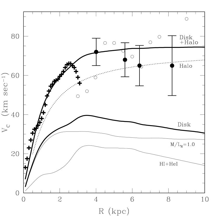
Figure 6: Same as Figures 4, except that the stellar rotation curve is now scaled with M/L=1.0, and we plot the contribution from a psuedo-isothermal dark halo (“Halo”) and the sum of the disk and halo curves (“Disk$+$Halo”).

In Figure 6, we present a “minimal” disk decomposition of the LMC rotation curve. We plot the same carbon star and H I data points as in Figures 4 and 5. We plot the stellar rotation curve assuming M/L = 1, the gas rotation curve, and the sum of the stellar and gas rotation curves. We also plot the contribution of a pseudo-isothermal dark halo, and the sum of the disk and halo rotation curves. In this decomposition, we calculate $M_{disk}=1.1\pm 1.0$ $\times$ $10^{9}M_{\odot}$ and $\Sigma_{0}=68$ $M_{\odot}$ pc^-2. The shallow and declining run of carbon star data points favors a small core radius for the LMC dark halo. The dark halo shown has $a$ = 1 kpc and $\rho_{0}$ = 0.10 $M_{\odot}$ pc^-3. By assuming M/L = 1 in the disk, this decomposition has a maximal halo, and yields a total LMC mass of $\sim$5 $\times$ $10^{9}M_{\odot}$ (corresponding to an upper limit on the LMC global mass-to-light ratio of $\sim$4).

5.2 Decomposition of the Disk Velocity Dispersions

In Figure 7, we plot our LMC disk velocity dispersions as a function of true radius with bold dots and error bars. We plot the results of KDIA with open circles (see also Fig. 1). The prediction of equation (8) for our maximal disk model is shown as a dotted line and labeled. We plot this model prediction again, but now corrected for the truncation of the LMC disk (the “$K_{Z}$ force correction”) as a bold solid line. We have assumed a constant scale height of $h=0.5$ kpc, which normalizes the latter curve to intersect the carbon star data point in the LMC bar. A constant-thickness disk model cannot be reconciled with the data by any choice of $h$.

For our minimal disk decomposition, we must account for the effect of the LMC dark halo on the disk velocity dispersions. By combining equations (6), (18), and (24), and equating $\rho_{halo}=\rho^{eff}_{halo}$, we may estimate the $\epsilon$ parameter,

$$\epsilon(R)=\frac{\rho_{0,halo}\left(1\ +\ \frac{R^{2}}{a^{2}}\right)^{-1}}{\rho_{0,disk}\ e^{-R/\Lambda}}$$ (33)

Assuming a constant scale height of $h=0.4$ kpc, the spatial density normalization of the minimal disk is $\rho_{0,disk}$ = 0.068 $M_{\odot}$ pc^-3. Adopting the parameters of the maximal LMC dark halo from above, we find $\epsilon\approx$ 1.1, 1.0, 1.2, 1.9 and 3.4 at integer steps of $R/\Lambda$ = 1 to 5. For these values of $\epsilon$, the error associated with equation (31) is too large, and thus we appeal directly to our numerical integrations in Table 5.

For this decomposition, we begin with the velocity dispersion according to equation (8), and then make the $K_{Z}$ force correction. We calculate $\epsilon(R)$ using equation (33), and use spline interpolations of the numerical data in Table 5 to calculate $\alpha$. The model disk velocity dispersions are corrected according to equation (29) by a factor of $\alpha^{-1}$ (equating $\sigma_{obs}=\sigma_{disk+halo}$). These various curves are plotted in Figure 8. Our choice of $h$ = 0.4 kpc normalizes the dark halo-corrected curve to intersect the data point in the LMC bar. A constant-thickness disk in the presence of a maximal dark halo cannot be reconciled with the observed velocity dispersions by any choice of $h$. For comparison, a fit to the velocity dispersion data with the minimal disk and an arbitrary pseudo-isothermal dark halo implies a maximum circular velocity in the rotation curve of $\sim$500 km s^-1, which is about 7 times higher than observed.

5.2.1 Scale Heights of the Carbon Stars

Our maximal disk model yields $h$ = 0.25, 0.93, and 1.62 kpc at $R$ = 0.5, 4.0, and 5.6 kpc, respectively. For comparison, the minimal disk yields $h$ = 0.55, 1.62, and 2.61 kpc at the same radii. At larger radii ($R>$ 6 kpc), where the disk velocity dispersions begin to rise, the implied scale heights for the maximal disk model are $h$ = 5.1 and 28.4 kpc (at $R$ = 6.5 and 8.2 kpc, respectively). The scale height inferred from the last data point is much larger than the tidal radius of the LMC (Weinberg 2000), and obviously wrong. We will return to the interpretation of these high velocity dispersions at large radii in a moment. A linear regression on the three data points with $R<6$ kpc yields:

$$\sigma(R)=-1.39\ (\pm 0.10)\times R\ +\ 22.89\ (\pm 0.42)$$ (34)

where $R$ is in units of kpc, and $\sigma(R)$ is in units of km s^-1. We adopt this regression to represent the flare of the LMC disk. The change of scale height is represented by a function of the form

$$h(R)\ =\ \kappa\ e^{+R/\beta\Lambda}$$ (35)

where $h$ and $R$ are in units of kpc. We find $\beta=1.4$, and $\kappa=0.14$ kpc. Equation (35) predicts the scale height to within 0.1 kpc of the values estimated above.

Assuming a constant mass-to-light ratio, our flared disk model must project to a surface density that varies as $e^{-R/\Lambda}$ in order to reproduce the observed surface brightness profile of the LMC (de Vaucouleurs 1957, Bothun & Thompson 1988). Therefore, the spatial density of the flared disk, $\rho_{f}(R)$, must change with an effective radial scale length that compensates for the variation of scale height with $R$. This effective radial scale length is easily calculated by considering

$$\Sigma(R)\ =\ \Sigma_{0}\ e^{-R/\Lambda}\ =\ 2\ \rho_{f}(R)\ h(R)\ =\ 2\ \rho_{0f}e^{-R/\gamma\Lambda}\ \kappa e^{+R/\beta\Lambda}$$ (36)

where we require that $(1/\gamma-1/\beta)=1$. Substituting $\beta$ = 1.4 yields $\gamma$ = 0.583 (note that $\gamma$ and $\beta$ are dimensionless scale factors). It also follows that $\rho_{0f}$ = $\Sigma_{0}/(2\kappa)$ = 1.064 $M_{\odot}$ pc^-3. In summary, our flared disk model has the following spatial density,

$$\rho_{f}(z,R)\ =\ \rho_{0f}\ e^{-R/\gamma\Lambda}\ {\rm sech}^{2}\left(\frac{z}{h(R)}\right)$$ (37)

where $h(R)$ is given in equation (35).

5.2.2 Dynamical Influence of the Galactic Dark Halo

The dynamical influence of the Galactic dark halo is calculated following the discussion in §4.2 of this paper (see also Aubourg et al. 1999). We designate the mean density of the Galactic dark halo at the distance of the LMC as $\overline{\rho}$. If we substitute $\overline{\rho}$ for $\rho_{eff}$ in equation (20), then $\epsilon$ from equation (24) yields $\alpha$ from Table 5, and thus the correction to the disk velocity dispersions through equation (29). We estimate $\overline{\rho}$ following Griest (1991; see his Eqn. [3]). We assume that the Galactic dark halo has a core radius of 3 kpc, and a solar neighborhood spatial density normalization of 0.0079 $M_{\odot}$ pc^-3. We adopt the distance from the Sun to the Galactic center of 8.5 kpc, and the distance from the Sun to the LMC of 50.1 kpc, which yields $\overline{\rho}$ = 0.00025 $M_{\odot}$ pc^-3. We estimate $\epsilon$ = 0.001, 0.007, 0.040, 0.224 and 1.246 at integer steps of $R/\Lambda$ = 1 to 5.

In Figure 9, we plot the same data points as in Figures 7 and 8. We indicate the regression of equation (34) as a solid line, and this regression corrected for the effect of the Galactic dark halo as a bold solid line. Although the fit is not perfect, the agreement with the last data point is quite good. Thus the influence of the Galactic dark halo on our flared disk model is of the correct magnitude to account for the outer-disk velocity dispersions. In addition, the radius where the Galactic dark halo begins to have a significant dynamical effect (i.e., where the velocity dispersions begin to rise in the disk) is also reasonably reproduced. A more detailed modeling of the outer-disk velocity dispersions is beyond the scope of this paper.

We find that $\epsilon$ is quite small at all radii of interest for the constant-thickness maximal disk model (accounting for the Galactic dark halo but no LMC dark halo), and for the constant-thickness minimal disk model (accounting for both the Galactic and LMC dark halos). In summary, constant-thickness exponential disk models cannot be reconciled with the observed run of LMC disk velocity dispersions.

As discussed above, we adopted the mean density of the Galactic dark halo at a distance of 50 kpc of $\overline{\rho}$ = 0.00025 $M_{\odot}$ pc^-3, or $\log\rho_{50}\sim-3.6$ (Griest 1991). It is worth considering the range of allowed Galactic dark halo profiles. Assuming flat rotation curves at large radii, many authors have made Galaxy models with pseudo-isothermal density profiles (e.g.  Caldwell & Ostriker 1981; Bahcall, Schmidt, & Soneira 1982). Typical core radii range from 2 to 8 kpc. The average value of the density at 50 kpc predicted by these models is $\log\rho_{50}=-3.6$, with a standard deviation of 0.2 dex. As a final check, we compare the N-body cold dark matter simulation of the Galactic dark halo presented by Dubinski (1994). The initial density profile for this dark halo model was similar to an ellipsoidal Hernquist potential, which is like the universal dark halo profile found in dark matter-dominated galaxies (Kravstov et al. 1998). Dubinski’s (1994) initial density profile was then compressed by the Galactic potential (e.g. Blumenthal et al. 1986) and in its final form predicts $\log\rho_{50}\sim-3.6$. The density profile of the Galactic dark halo assumed for MACHOs (Alcock et al. 2000) is also pseudo-isothermal; thus our analysis of the LMC disk kinematics supports this dark halo profile over the range of interest ($\sim 8$ to 50 kpc).

5.2.3 Tidal Debris?

It has been suggested that the LMC is embedded in a “shroud” of tidal debris (Weinberg 2000). Such debris is unlikely to contribute significantly to the LMC self-lensing optical depth because too little mass is involved, and it is likely to be located close to the disk (Weinberg 2000; see §6.2). Nonetheless, it is worth considering the possibility that our sample of true disk carbon stars is contaminated by tidal debris, which might reconcile a constant-thickness disk model with the disk kinematic data. In this case, tidal debris would also affect our interpretation of the outer-disk velocity dispersions. The notion of tidal debris surrounding the LMC is somewhat similar to the suggestion by KDIA that the LMC harbors a polar ring, also of tidal origin. (We note that KDIA analysed a larger sample of carbon stars, in which they claim the kinematic signature of a polar ring is evident.) We have thus far presented an interpretation of the radial velocity data for 422 carbon stars in the LMC that does not require a polar ring, or tidal debris. The nature of tidal debris (in a polar ring or otherwise) is investigated as follows.

If we assume that a constant-thickness maximal disk model represents the true LMC disk, the “excess” velocity dispersion in each zonal solution may be calculated by subtracting the model contribution from the observed dispersions in quadrature, which yields $\sigma_{ex}$ = 15.0, 13.7, 18.8 and 20.5 km s^-1 at $R$ = 4.0, 5.6, 6.4 and 8.2 kpc, respectively. Next, if we assume that the contaminating debris has a uniform velocity dispersion of $\sim$50 km s^-1, the ratio of contaminating stars to total stars in each zonal solution would be of order $\sim$10-20%. (This ratio is inversely proportional to the velocity dispersion assumed for the tidal debris.) In each of our zones, we estimate the number of $\sim$50 km s^-1 tidal debris stars would be 12, 17, 10, and 8 (in order of increasing radius), if the LMC disk were of constant thickness.

We calculate that our four disk zones subtend relative sky areas of 0.40/0.16/0.16/1.00, in order of increasing zone radius. A regression of the relative numbers of tidal debris stars with the relative zone areas shows an anti-correlation, significant at the $\sim$1$\sigma$ level. Assuming that the true disk and tidal debris carbon stars are similarly affected by incompleteness in the data, this is not what we naively expect from the tidal debris scenario described by Weinberg (2000). The two outermost zones are illustrative. They have area ratios that differ by a factor of $\sim$6, yet the estimated numbers of contaminating tidal debris stars are 10 and 8. Therefore, the contaminating debris must have a non-uniform radial distribution of surface density, velocity dispersion, or both. It is also possible, but even more contrived, that a spatially-dependent incompleteness in the carbon star dataset has conspired with a non-uniform spatial distribution of tidal debris to yield the observed velocity dispersions. In light of this analysis, we prefer an interpretation of the LMC rotation curve and disk velocity dispersions that invokes a negligible contamination from tidal debris (i.e., our maximal flared disk model).

The unambiguous detection of nonvirialized LMC stars and the accurate characterization of their spatial distribution are clearly desirable. Observations of such a population/structure would be relevant to our interpretation of the LMC rotation curve and disk kinematics, with possible additional implications for LMC microlensing (e.g. Zhao 1999; Graff et al. 1999; Weinberg 2000).

6 Microlensing Implications

6.1 Self-Lensing of the Flared LMC Disk

Here we calculate the LMC self-lensing optical depth of our maximal flared disk model by directly integrating the spatial density of stars given in equation (37). We begin with an integral of the form

$$\tau(R_{s},\phi_{s},z_{s})=\frac{4\pi G}{c^{2}}\ \int\limits^{D_{s}}\limits_{0}\rho(y)\ \left(1-\frac{y}{D_{s}}\right)\ y\ dy\approx\frac{4\pi G}{c^{2}}\ \int\limits^{D_{s}}\limits_{0}\rho(y)\ y\ dy$$ (38)

which yields the optical depth to any source star in the LMC at position $(R_{s},\phi_{s},z_{s})$, a cylindrical coordinate system in the plane of the disk. The position angle $\phi$ is defined to be zero at the near side if the inclined disk. The integration variable is the line of sight distance between the source and lens. We use the subscripts “$s$” and “$l$” to denote the coordinates of the sources and lenses, respectively. The approximation in equation (38) is that $y$ is always much smaller than the distance to the source ($D_{s}\approx$ 50.1 kpc), which is reasonable for LMC self-lensing. Note that $y$ is simply related to $D_{l}$, the distance from the observer to the lens, and $D_{s}$, the distance from the observer to the source

$$y=D_{l}-D_{s}=\frac{z_{l}-z_{s}}{\cos~{}i}$$ (39)

where $i$ is the inclination angle of the disk (measured from the plane of the sky). For completeness, we provide the following geometric identity relating the source and lens positions to $y$:

$$R_{l}^{2}\ =\ R_{s}^{2}\ +\ y^{2}\sin^{2}i\ +\ 2R_{s}y\cos~{}\phi_{s}$$ (40)

It is necessary to integrate over the line of sight a second time, in order to calculate a density-weighted average of $\tau(R_{s},\phi_{s},z_{s})$ over the distribution of source stars

$$\overline{\tau}(R,\phi)\ =\ \frac{\int\limits^{\infty}\limits_{0}\rho(R_{s},z_{s})\ \tau(R_{s},\phi_{s},z_{s})\ dD_{s}}{\int\limits^{\infty}\limits_{0}\rho(R_{s},z_{s})\ dD_{s}}$$ (41)

which may be properly compared to the observed optical depth. The integration over $D_{s}$ is made in practice by transforming to a variable in our LMC cylindrical coordinate system (i.e., $dD_{s}=dz_{s}/\cos~{}i$). We truncate the LMC disk at a conservative radius of 10 kpc. Our results are insensitive to the choice of truncation radius at the few percent level. We calculate $\overline{\tau}(R,\phi)$ for multiple lines of sight, designated by ($R,\phi$) in the plane of the disk. Our calculation is the case of “pure” self-lensing (Gould 1995), which yields an upper limit. The effects of dust obscuration and nonlensing mass in the plane of the disk will lower the real value of the optical depth for a fixed total mass of the LMC.

We have calculated the self-lensing optical depths in each of the 30 survey fields in the 5.7-year LMC microlensing analysis by Alcock et al. (2000; see also Gyuk et al. 1999). In the central-most fields, we find $\overline{\tau}\approx\ 1.7\times 10^{-8}$, while in the fields lying at the largest true radii, we find $\overline{\tau}\approx\ 1.2\times 10^{-8}$. The field-averaged optical depth for LMC disk self-lensing is: $\overline{\tau}_{30}\ =\ 1.4\times 10^{-8}$.

The LMC inclination dominates the uncertainty in $\overline{\tau}_{30}$. First, we note that the inclination is probably not a serious concern for the rotation curve and disk kinematics because the shape of the $V(\Theta)$ function (Eqn. [15]) is fairly insensitive to $i$ over the range of plausible values. However, Gould (1995) and Gyuk et al. (1999) show that, to first order, $\tau$ is proportional to the square of the mass-weighted velocity dispersion and an inclination factor of sec${}^{2}i$. Therefore, we simply rescale our calculation of $\overline{\tau}_{30}$ for different inclinations,

$$\overline{\tau}_{30}\ <\ 1.0\times 10^{-8}\cdot\sec^{2}i\\$$ (42)

which should be quite accurate for the LMC inclinations typically found. As noted in §2.2, Cole et al. (1999) find $i=36^{+2}_{-5}$. Thus their $\sim$2$\sigma$ upper limit, $i<38$, yields $\overline{\tau}_{30}<1.6\times 10^{-8}$. For comparison, Bothun & Thompson (1988) find $i=45$, which corresponds to $\overline{\tau}_{30}<2.0\times 10^{-8}$. The contribution to the uncertainty in $\overline{\tau}_{30}$ from the velocity dispersion follows from Gould’s (1995) formula and our equation (34); it is of order $\sim(0.42/22.89)^{2}$, or a negligible 0.03%. Finally, the $\sim$10% uncertainty in $V_{C}$ yields a $\sim$20% uncertainty on the total LMC mass, but this corresponds to a small uncertainty in the factor of $1.0\times 10^{-8}$ in equation (42).

The self-lensing optical depth on the near and far sides of the minor axis at the distances spanned by the 30 fields in Alcock et al. (2000) varies by $\sim$5% due to the inclination of the disk (e.g. Gould 1994). Thus the flaring of the LMC disk has only a minor effect on the spatial distribution of the self-lensing optical depth, which is a potential diagnostic of the lens population (e.g. Alcock et al. 2000). The estimate of a $\sim$5% minor axis asymmetry in the optical depth would increase for larger adopted values of the inclination.

6.2 Discussion of LMC Self-Lensing

Gyuk et al. (1999) recently reviewed different self-lensing calculations in the literature. To first order, self-lensing from the virialized LMC disk is proportional to the following combinations of derivable quantities (Gyuk et al. 1999),

$$\tau\ \ \propto\ \ \left(\frac{M_{disk}\ h}{\Lambda^{2}}\right)\sec^{2}i\ \ \propto\ \ \sigma^{2}\sec^{2}i$$ (43)

Our model accounts for “second order” effects, such as the finite radial extent and flare of the LMC disk. We have shown that uncertainties in the LMC proper motion contribute a $\sim$1% uncertainty to $\sigma$ and a $\sim$20% uncertainty to $M_{disk}$ (via $V_{C}$), assuming a truncated and flared maximal disk model. Assuming this model, our numerical calculation of the self-lensing optical depth (Eqn. [42]) is appropriate.

The maximal disk model is consistent with LMC dynamics. However, if a model of the LMC with a dark halo is preferred, the halo will probably contribute to LMC self-lensing in addition to the disk. In this case, our equation (42) is not appropriate (see Gyuk et al. 1999). We have adopted a minimal LMC disk, and provided an example maximal dark halo which is consistent with the rotation curve. Measurements of the LMC disk mass to light ratio would better constrain the minimal LMC disk model (our model is extreme). For the more complicated case of an LMC with a dark halo, constraints on self-lensing are weaker. This is due partly to the uncertainty that the LMC proper motion contributes to the rotation curve, which constrains the total LMC mass.

The LMC self-lensing optical depth may depend systematically on the age of the stars whose kinematics are studied. Historically, it has been difficult to prove that old LMC stellar populations have different velocity dispersions. For example, the CH stars in the LMC were originally thought to trace the elusive LMC halo population, by analogy with CH stars in the Galaxy (Hartwick & Cowley 1988, Cowley & Hartwick 1991). However, the CH stars in the LMC are now believed to represent a much younger population (Suntzeff et al. 1993). We note that our average carbon star velocity dispersion (18.9 km s^-1) is similar to that found for the CH stars (20 km s^-1).

According to Aubourg et al. (1999) and Salati et al. (1999), the LMC could harbor an old population with a large velocity dispersion. These authors invoke Wielen’s (1977) age-velocity dispersion calibration from the solar neighborhood. We note that Weilen’s calibration was derived for stars younger than $\sim$3 Gyr, and extrapolation beyond this age may not be appropriate. Moreover, Weinberg (2000) predicts that the velocity dispersions in the LMC disk, under the influence of the Galactic tidal field, will remain constant (or decrease) over time.

Extant observational studies have not yielded a clear picture of the variation of velocity dispersion with age in the LMC. For example, the old globular clusters in the LMC, with ages of $\sim$12 Gyrs (Olsen et al. 1998), exhibit a velocity dispersion of $\sim$21-24 km s^-1 (Schommer et al. 1992; see also Freeman, Illingworth, & Oemler 1982). Thus, the LMC carbon stars and ancient clusters support the hypothesis of a constant disk velocity dispersion (for stellar populations older than $\sim$3 Gyr), in agreement with Weinberg’s (2000) prediction. However, the velocity dispersion of old LPVs in the LMC, with ages of $\sim$8 Gyr (Hughes, Wood, & Reid 1991; Olszweski, Sunzteff, & Mateo 1996), is $\sim$35 km s^-1 (Hughes et al. 1991). Further observational studies are needed, particularly given the provocative old LPV result.

Last, we suggest that a shroud of tidal debris or a polar ring, if they exist, would probably make a negligible contribution to the LMC self-lensing optical depth because the total amount of mass involved is small. Weinberg (2000) reached a similar conclusion.

7 Conclusion

The rotation of the disk of the LMC has been derived from the radial velocities of 422 carbon stars (Kunkel, Irwin, & Demers 1997). We have propogated the uncertainty in the LMC space motion to the LMC rotation curve with a Monte Carlo calculation. The associated disk velocity dispersions found in each rotating disk zonal solution are less sensitive to systematic uncertainties from the LMC space motion than the circular velocities obtained. We note that our carbon star rotation curve is derived in a manner consistent with the H I rotation curve analysis by Kim et al. (1998); thus our respective results are properly comparable.

We have fit our carbon star rotation curve and the H I rotation curve with a truncated, maximal LMC disk model, yielding a total LMC mass of $5.3\pm 1.0$ $\times$ $10^{9}M_{\odot}$. We also conclude that the disk of the LMC is flared. Extrapolating the flare inferred at small radii (where tidal perturbations are small) to the outer-disk, and accounting for the influence of the Galactic dark halo, we are able to approximately reproduce the observed disk kinematics. This model favors an isothermal density profile for the Galactic dark halo out to a distance of 50 kpc. Our truncated and flared maximal disk model yields a limit on the spatially-averaged LMC self-lensing optical depth of $\overline{\tau}_{30}\ <\ 1.0\times 10^{-8}\cdot\sec^{2}i$. For plausible values of the LMC inclination, this low self-lensing rate compared to the measured microlensing rate allows for the existence of a dark lens population in the Galactic halo (Alcock et al. 2000).

Finally, we caution that we have not included in our analysis (1) the dynamical effects of an LMC bar, (2) large-scale non-circular motions, (3) non-uniform anisotropy of the disk velocity dispersions, or (4) arbitrary spatial distributions of tidal debris (i.e., a polar ring or stars out of virial equilibrium). Despite these shortcomings, our truncated and flared maximal disk model successfully accounts for the general dynamical characteristics of the LMC, lending inferences from the model high weight.

8 Acknowledgments

D.R.A. acknowledges Howard E. Bond for support of work performed at the Space Telescope Science Institute, and Kem H. Cook for support of work performed at the Lawrence Livermore National Laboratory. NASA Research Grant NAG5-6821 “UV, Visible, and Gravitational Astrophysics Research and Analysis” and DOE Contract W7405-ENG-48 are recognized. C.A.N. acknowledges support from National Physical Science Consortium Graduate Student Fellowship. We thank Ken Freeman, David Bennett, Tim Axelrod, Howard Bond, Kailash Sahu, Geza Gyuk, Greg Bothun, and the anonymous referee for their helpful discussions and comments.

Figure 1: Velocity dispersion of carbon stars in the LMC as a function of radius. Data taken from Kunkel, Demers, Irwin and Albert (1997; KDIA). Solid line shows the prediction for an exponential disk model. Dashed line shows the prediction for a flared disk model.

Figure 2: Distribution of LMC carbon stars with archival radial velocities (open circles) in coordinates $\alpha$ and $\delta$ (1950 right ascension & declination in units of radians). The bold dot indicates the kinematic center of the LMC.

Figure 3: LMC rotation curve solutions derived from carbon star radial velocity data (open circles). Each of the four panels corresponds to a different radial zone. Each carbon star is plotted twice, at $\theta$ and $\theta+2\pi$ for clarity. The best fit rotating disk model is shown as a solid line through the data. The amplitude corresponds to the circular velocity. The circular velocity and velocity dispersion (km s^-1), and mean radius of the carbon stars (kpc) are also labeled.

Figure 4: The LMC rotation curve: circular velocity in km s^-1 versus true radius in kpc. The H I data of Kim et al. (1999) are plotted with crosses. The carbon star results of KDIA are shown as small open circles. Our four zonal solutions are shown as filled circles, with standard errorbars. We plot the gas (“H I$+$He I”), stellar (“M/L=2.2”), and sum of gas and stellar rotation curves (“Disk”).

Figure 5: Same as Figure 4, expect that the finite-thickness, truncated model disk rotation curve (“$V_{MAX}$=71”) has been substituted for the stellar rotation curve.

Figure 7: We plot the run of LMC disk velocity dispersion with radius (km s^-1 versus kpc). Our points are bold dots with errorbars. The solutions of KDIA are shown as open circles (errorbars omitted for clarity). We show the predicted curve for our maximal LMC disk model (see also Fig. 4) as a dotted line, and this curve properly corrected for the finite extent of the disk as a bold solid line. This curve has been normalized ($h=0.5$ kpc) to intersect the point at $R=0.5$ kpc.

Figure 8: Same as Figure 7, except that we show the prediction for our minimal LMC disk model (dotted line), this model but corrected for the finite extent of the LMC (solid line), and finally this disk model but with the effect of a psuedo-isothermal dark halo also included (bold dashed line).

Figure 9: Same as Figures 7 and 8, except that we show the prediction for our maximal flared LMC disk model (solid line), and this model corrected for the effect of the Galactic dark halo (bold solid line).

1cm Zone N $<R>$ $\theta_{0}$ $V$ $\sigma_{V}$ (kpc) (kpc) (deg.) (km s^-1) (km s^-1) 2.5 - 5.0 91 4.0 $-37$ 72 $\pm$ 7.1 17.6 $\pm$ 0.3 5.0 - 6.0 139 5.6 $-22$ 68 $\pm$ 8.7 14.9 $\pm$ 0.2 6.0 - 7.0 122 6.4 $-8$ 65 $\pm$ 10.4 19.3 $\pm$ 0.4 7.0 - 13.0 73 8.2 3 65 $\pm$ 15.8 20.6 $\pm$ 0.5

Table 1: Carbon Star Rotating Disk Solutions

1cm R $V_{disk}$ $V_{disk}$ R $V_{disk}$ $V_{disk}$ $M/L_{R}$=1.0 $M/L_{R}$=2.2 $M/L_{R}$=1.0 $M/L_{R}$=2.2 (kpc) (km s^-1) (km s^-1) (kpc) (km s^-1) (km s^-1) 0.5 14.0 30.8 5.5 28.6 62.7 1.0 23.5 51.7 6.0 28.3 62.1 1.5 28.6 62.7 6.5 28.0 61.5 2.0 30.8 67.7 7.0 28.0 61.5 2.5 31.4 68.9 7.5 28.0 61.5 3.0 31.4 68.9 8.0 27.7 60.9 3.5 31.4 68.9 8.5 27.4 60.3 4.0 30.8 67.7 9.0 27.4 60.3 4.5 30.2 66.4 9.5 27.4 60.3 5.0 29.1 64.0 10.0 27.2 59.7

Table 2: Stellar Disk Rotation Curve

1cm R/$\Lambda$ $V_{disk}$/$V_{max}$ R/$\Lambda$ $V_{disk}$/$V_{max}$ 0.5 0.550 3.5 0.900 1.0 0.780 4.0 0.890 1.5 0.900 4.5 0.820 2.0 0.950 5.0 0.750 2.5 0.955 5.5 0.700 3.0 0.945 6.0 0.650

Table 3: Model Disk Rotation Curve

1cm R $V_{disk}$ R $V_{disk}$ (kpc) (km s^-1) (kpc) (km s^-1) 0.5 5.0 5.5 22.8 1.0 9.0 6.0 22.5 1.5 10.0 6.5 21.0 2.0 12.0 7.0 20.0 2.5 16.0 7.5 19.0 3.0 22.0 8.0 18.5 3.5 24.2 8.5 17.0 4.0 23.8 9.0 16.0 4.5 23.0 9.5 15.0 5.0 23.0 10.0 14.5

Table 4: Gas Contribution to Rotation Curve

cm $\epsilon$ $\alpha$ $\epsilon$ $\alpha$ 0.000 1.000 6.000 0.339 0.250 0.865 7.000 0.317 0.500 0.776 8.000 0.298 1.000 0.658 9.000 0.283 1.500 0.582 10.000 0.269 2.000 0.528 12.000 0.248 2.500 0.486 15.000 0.223 3.000 0.453 20.000 0.194 4.000 0.404 30.000 0.160 5.000 0.367 50.000 0.124

Table 5: Epsilon and Alpha Integrations

References

- (1) Alcock, C., et al. 1997, ApJ, 490, L59
- (2) Alcock, C., et al. 2000, astroph/0001272
- (3) Alcock, C., et al. 2000b, astroph/0001435
- (4) Aubourg, E. et al. 1999, A&A, 347, 850
- (5) Bahcall, J.N. 1984, ApJ, 276, 156
- (6) Bahcall, J.N., Schmidt, M., & Soneira, R.M. 1982, ApJ, 258, 623
- (7) Bahcall, J.N. & Casertano, S. 1984, ApJ, 284, L35
- (8) Bahcall, J.N., Flynn, C. & Gould, A. 1992, 339, 234
- (9) Barrow, J.D., Sonoda, D.H., & Bhasvar, S.P. 1984, MNRAS 210, p19
- (10) Beaulieu, J-P. & Sackett, P. 1998, AJ, 116, 209
- (11) Bennett, D.P. 1998, ApJ, 439, 79
- (12) Blumenthal, G.R., Faber, S.M., Flores, R., & Primack, J. 1986, ApJ, 301, 27
- (13) Bothun, G.D., & Thompson, I.B. 1988, AJ, 96, 877
- (14) Bottema, R. 1993, A&A, 16, 36
- (15) Caldwell, J.A.R. & Ostriker, J.P. 1981, ApJ, 251, 61
- (16) Cole, A., Wood, K., & Nordsieck, K.H. 1999, AJ, 118, 2292
- (17) Cowley, A.P & Hartwick, F.D. 1991 ApJ, 373, 80
- (18) de Grijs, R., Peletier, R.F. & van der Kruit, P.C. 1997, A&A, 327, 966
- (19) de Vaucouleurs, G. 1957, AJ, 62, 69
- (20) Dubinski, J. 1994, ApJ, 431, 617
- (21) Evans, W.F. & Kerins, E. 2000, ApJ, 529, 917
- (22) Evans, W.F., Gyuk, G., Turner, M. & Binney, J. 1998, ApJ, 501, L45
- (23) Feast, M.W., Thackeray, A.D. & Wesselink, A.F. 1961, MNRAS, 122, 433
- (24) Freeman, K.C. 1970, ApJ, 160, 811
- (25) Freeman, K.C., Illingworth, G. & Oemler,A. 1983, ApJ, 272, 488
- (26) Gould, A. 1994, ApJ, 435, 573
- (27) Gould, A. 1995, ApJ, 441, 77
- (28) Gould, A. 1998, ApJ, 499, 728
- (29) Gould, A. 1999, ApJ, 525, 734
- (30) Griest, K. 1991, ApJ, 366, 412
- (31) Graff, D., et al. 1999, astroph/9910360
- (32) Gyuk, G., Flynn, C. & Evans, W.F. 1999, ApJ, 521, 190
- (33) Gyuk, G., Dalal, N. & Griest, K. 1999, astroph/9907338
- (34) Hartwick, F.D. & Cowley, A.P, 1988 ApJ, 334, 135
- (35) Hughes, S.M., Wood, P.R., & Reid, N. AJ, 101, 1304
- (36) Ibata, R., Geraint, L. & Beaulieu, J-P. 1998, ApJ, 509, L29
- (37) Johnston, K. 1998, ApJ, 495, 297
- (38) Jones, B.F., Klemola, A.R. & Lin, D.N.C. 1994, AJ, 107, 1333
- (39) Kim, S. et al. 1998, ApJ, 503, 674
- (40) Kravstov, A.V., Klypin, A.D., Bullock, J.S., & Primack, J.R. 1998, ApJ, 502, 48
- (41) Kroupa, P. & Bastian, U. 1997, New Ast., 2, 77
- (42) Kunkel, W.E., Irwin, M.J., & Demers, S. 1997, A&AS, 122, 463
- (43) Kunkel, W.E., Demers, S., Irwin, M.J., & Albert, L. 1997, ApJ, 488, L129 (KDIA)
- (44) Lewis, J.R. & Freeman, K.C. 1989, AJ, 97, 139
- (45) Luks, T. & Rohlfs, K. 1992, A&A, 263, 41
- (46) Meatheringham, S.J., Dopita, M., Ford, H., & Webster, B.L. 1988, ApJ, 327, 651
- (47) Olszewski, E., Suntzeff, N., & Mateo, M. 1996 ARA&A, 34, 511
- (48) Olsen, K.A.G., et al. 1998, MNRAS, 300, 665
- (49) Paczýnski, B. 1986, ApJ, 304, 1
- (50) Sahu, K. 1994, Nature, 370, 275
- (51) Salati, P., et al. 1999, A&A, 350, L57
- (52) Schommer, R.A., Olszewski, E., Suntzeff, N., & Harris, H. 1992, AJ, 103, 447
- (53) Spitzer, L. 1942, ApJ, 95, 329
- (54) Suntzeff, N. et al. 1993, PASP, 105, 350
- (55) Suntzeff, N. 1998, private communication
- (56) van der Kruit, P.C. 1988, A&A, 192, 117
- (57) van der Kruit, P.C. & Searle, L. 1981, A&A, 95, 116
- (58) van der Kruit, P.C. & Searle, L. 1981b, A&A, 105, 115
- (59) van der Kruit, P.C. & Searle, L. 1982, A&A, 110, 61
- (60) van der Kruit, P.C. & Freeman, K.C. 1984, ApJ, 278, 81
- (61) Wainscoat, R.J, Freeman, K.C., & Hyland, A.R. 1989, ApJ, 337, 163
- (62) Weinberg, M.D. 2000, ApJ, 532, 922
- (63) Westerlund, B.E. 1997, “The Magellanic Clouds” (Cambridge: Cambridge University Press)
- (64) Wielen, R. 1977, A&A, 60, 263
- (65) Wu, X-P. 1994, ApJ, 435, 66
- (66) Zaritsky, D. & Lin, D. 1997 AJ, 114, 254
- (67) Zaritsky, D., et al. 1999 AJ, 117, 2268
- (68) Zhao, H., 1998, MNRAS, 294, 139
- (69) Zhao, H., 1999, ApJ, 526, 141
- (70)