The Sun’s acoustic asphericity and magnetic fields in the solar convection zone

Abstract

The observed splittings of solar oscillation frequencies can be employed to separate the effects of internal solar rotation and to estimate the contribution from a large-scale magnetic field or any latitude-dependent thermal perturbation inside the Sun. The surface distortion estimated from the rotation rate in the solar interior is found to be in good agreement with the observed oblateness at solar surface. After subtracting out the estimated contribution from rotation, there is some residual signal in the even splitting coefficients, which may be explained by a magnetic field of approximately 20 kG strength located at a depth of 30000 km below the surface or an equivalent aspherical thermal perturbation. An upper limit of 300 kG is derived for a toroidal field near the base of the convection zone.

1 Introduction

Rotational splittings of solar oscillation frequencies have been successfully utilized to infer the rotation rate in the solar interior. To first order, rotation affects only the splitting coefficients which represent odd terms in the azimuthal order $m$ of the global resonant modes. The even terms in these splitting coefficients, which reflect the Sun’s effective acoustic asphericity, can arise from second order effects contributed both by the rotation and magnetic field as also from latitudinal temperature variations. Since the rotation rate can be inferred using the odd splitting coefficients, the inferred profile can be used to estimate the second order effects. These can then be subtracted from the observed even coefficients to estimate the magnetic field strength (Gough & Thompson 1990) or other latitudinal variations in sound propagation speed. The distortion introduced by rotation can be compared with the measured oblateness at the solar surface.

The even coefficients of splittings are fairly small, and no definitive results have so far been obtained regarding the magnetic field strength in the solar interior. With the good quality data now becoming available from GONG (Global Oscillation Network Group) and MDI (Michelson Doppler Imager) projects, it is desirable to investigate the possibility of inferring the strength of magnetic field in solar interior. There should also be some shift in the mean frequency for each $n,\ell$ multiplet due to second order effects from rotation and magnetic field, which can also be estimated. It is difficult to measure this frequency shift from observed data as it is hard to separate it from the effects of other uncertainties in the spherical structure of the Sun. Nevertheless, these frequency shifts can affect the helioseismic inferences and it would be interesting to estimate their effect.

2 The technique

The frequencies of solar oscillations can be expressed in terms of the splitting coefficients:

$$\nu_{n,\ell,m}=\nu_{n,\ell}+\sum_{j=1}^{J_{\rm max}}a_{j}^{n,\ell}{\cal P}_{j}^{\ell}(m),\qquad\qquad(J_{\rm max}\leq 2\ell)$$ (1)

where ${\cal P}_{j}^{\ell}(m)$ are orthogonal polynomials of degree $j$ in $m$ (Ritzwoller & Lavely 1991; Schou, Christensen-Dalsgaard & Thompson 1994). The odd coefficients $a_{1},a_{3},a_{5},\ldots$ can be used to infer the rotation rate in the solar interior, while the even coefficients arise basically from second order effects due to rotation and magnetic field. Since forces due to rotation or magnetic field in the solar interior are smaller by about 5 orders of magnitude as compared to gravitational forces, it is possible to apply a perturbative treatment to calculate their contribution to frequency splittings. In this approach, we estimate the effects of rotation and magnetic field on the frequencies but without explicitly constructing a model of a rotating, magnetic star.

We adopt the formulation due to Gough & Thompson (1990), with the difference that we include perturbation in the gravitational potential and also assume differential rotation in the interior, though the symmetry axis of magnetic field is taken to coincide with rotation axis.

In an inertial frame the oscillation equations can be formally written as

$${\cal L}\kern-0.15pt\hbox{$\xi$}\kern-4.37502pt\kern 0.29999pt\hbox{$\xi$}\kern-4.37502pt\kern-0.15pt\raise 0.29999pt\hbox{$\xi$}+\rho\omega^{2}\kern-0.15pt\hbox{$\xi$}\kern-4.37502pt\kern 0.29999pt\hbox{$\xi$}\kern-4.37502pt\kern-0.15pt\raise 0.29999pt\hbox{$\xi$}=\omega{\cal M}\kern-0.15pt\hbox{$\xi$}\kern-4.37502pt\kern 0.29999pt\hbox{$\xi$}\kern-4.37502pt\kern-0.15pt\raise 0.29999pt\hbox{$\xi$}+{\cal N}\kern-0.15pt\hbox{$\xi$}\kern-4.37502pt\kern 0.29999pt\hbox{$\xi$}\kern-4.37502pt\kern-0.15pt\raise 0.29999pt\hbox{$\xi$}+{\cal B}\kern-0.15pt\hbox{$\xi$}\kern-4.37502pt\kern 0.29999pt\hbox{$\xi$}\kern-4.37502pt\kern-0.15pt\raise 0.29999pt\hbox{$\xi$},$$ (2)

where

$${\cal L}\kern-0.15pt\hbox{$\xi$}\kern-4.37502pt\kern 0.29999pt\hbox{$\xi$}\kern-4.37502pt\kern-0.15pt\raise 0.29999pt\hbox{$\xi$} = \nabla(\rho c_{s}^{2}\nabla\cdot\kern-0.15pt\hbox{$\xi$}\kern-4.37502pt\kern 0.29999pt\hbox{$\xi$}\kern-4.37502pt\kern-0.15pt\raise 0.29999pt\hbox{$\xi$}+\kern-0.15pt\hbox{$\xi$}\kern-4.37502pt\kern 0.29999pt\hbox{$\xi$}\kern-4.37502pt\kern-0.15pt\raise 0.29999pt\hbox{$\xi$}\cdot\nabla p)-(\nabla\cdot\kern-0.15pt\hbox{$\xi$}\kern-4.37502pt\kern 0.29999pt\hbox{$\xi$}\kern-4.37502pt\kern-0.15pt\raise 0.29999pt\hbox{$\xi$}+\kern-0.15pt\hbox{$\xi$}\kern-4.37502pt\kern 0.29999pt\hbox{$\xi$}\kern-4.37502pt\kern-0.15pt\raise 0.29999pt\hbox{$\xi$}\cdot\nabla\ln\rho)\nabla p$$ (3)

$$\qquad-\rho G\nabla\left(\int{\nabla\cdot(\rho\kern-0.15pt\hbox{$\xi$}\kern-4.37502pt\kern 0.29999pt\hbox{$\xi$}\kern-4.37502pt\kern-0.15pt\raise 0.29999pt\hbox{$\xi$})\over|{\bf r}-{\bf r}^{\prime}|}d^{3}{\bf r}^{\prime}\right),$$

$${\cal M}\kern-0.15pt\hbox{$\xi$}\kern-4.37502pt\kern 0.29999pt\hbox{$\xi$}\kern-4.37502pt\kern-0.15pt\raise 0.29999pt\hbox{$\xi$} = -2i\rho{\bf v}\cdot\nabla\kern-0.15pt\hbox{$\xi$}\kern-4.37502pt\kern 0.29999pt\hbox{$\xi$}\kern-4.37502pt\kern-0.15pt\raise 0.29999pt\hbox{$\xi$},$$ (4)

$${\cal N}\kern-0.15pt\hbox{$\xi$}\kern-4.37502pt\kern 0.29999pt\hbox{$\xi$}\kern-4.37502pt\kern-0.15pt\raise 0.29999pt\hbox{$\xi$} = -\rho\kern-0.15pt\hbox{$\xi$}\kern-4.37502pt\kern 0.29999pt\hbox{$\xi$}\kern-4.37502pt\kern-0.15pt\raise 0.29999pt\hbox{$\xi$}\cdot\nabla({\bf v}\cdot\nabla{\bf v})+\rho({\bf v}\cdot\nabla)^{2}\kern-0.15pt\hbox{$\xi$}\kern-4.37502pt\kern 0.29999pt\hbox{$\xi$}\kern-4.37502pt\kern-0.15pt\raise 0.29999pt\hbox{$\xi$},$$ (5)

$${\cal B} = -{1\over 4\pi}\left({\nabla\cdot(\rho\kern-0.15pt\hbox{$\xi$}\kern-4.37502pt\kern 0.29999pt\hbox{$\xi$}\kern-4.37502pt\kern-0.15pt\raise 0.29999pt\hbox{$\xi$})\over\rho}(\nabla\times{\bf B})\times{\bf B}+(\nabla\times{\bf B}_{1})\times{\bf B}\right.$$ (6)

$$\left.\phantom{\nabla\cdot(\rho\kern-0.15pt\hbox{$\xi$}\kern-4.37502pt\kern 0.29999pt\hbox{$\xi$}\kern-4.37502pt\kern-0.15pt\raise 0.29999pt\hbox{$\xi$})\over\rho}+(\nabla\times{\bf B})\times{\bf B}_{1}\right).$$

Here ${\bf B}_{1}=\nabla\times(\kern-0.15pt\hbox{$\xi$}\kern-4.37502pt\kern 0.29999pt\hbox{$\xi$}\kern-4.37502pt\kern-0.15pt\raise 0.29999pt\hbox{$\xi$}\times{\bf B})$ is the linearized Eulerian perturbation to magnetic field, ${\bf B}$, $\xi$$\xi$$\xi$ is the displacement eigenfunction, ${\bf v}=\kern-0.15pt\hbox{$\Omega$}\kern-7.22223pt\kern 0.29999pt\hbox{$\Omega$}\kern-7.22223pt\kern-0.15pt\raise 0.29999pt\hbox{$\Omega$}\times{\bf r}$ is the velocity due to rotation, and $p,\rho,c_{s}$ are respectively, pressure, density and sound speed in the equilibrium state.

In the presence of rotation and magnetic field the equilibrium state will naturally undergo a distortion that needs to be included in the calculations. To account for this deformation we consider a transformation to map each point $\bf r$ in the distorted star to a point $\bf x$ in the spherical volume occupied by the undistorted star by a transformation

$$x=(1+h_{\Omega}({\bf r})+h_{B}({\bf r}))r,$$ (7)

where the functions $h_{\Omega}({\bf r})$ and $h_{B}({\bf r})$ which depend on the rotation and magnetic field respectively, are to be determined by solving the equations for equilibrium in a distorted star (Gough & Thompson 1990). This will give us the perturbation to a nonrotating spherically symmetric solar model and the extent of distortion at the surface may be compared with observed values. Here, $x$ is chosen so that $x=R$ can be regarded as the distorted solar surface, where $R$ is the radial distance of the outermost layer included in the solar model. Similarly, various equilibrium quantities are also expressed in the form

$$\rho(r)=\rho_{0}(x)+\rho_{\Omega}({\bf x})+\rho_{B}({\bf x}).$$ (8)

In all these expansions higher order terms have been neglected.

We consider the terms on the right hand side of Eq. 2, as perturbations to basic equations for linear adiabatic oscillations for non-magnetic and non-rotating star. Rotation introduces a first order perturbation through ${\cal M}$ which gives the odd splitting coefficients, while magnetic field can only give rise to even terms in $m$ and contributes to the even splitting coefficients. The distortion from a spherically symmetric equilibrium state also introduces even order terms. The relative magnitude of contributions from rotation and magnetic field will, of course, depend on the rotation rate and magnetic field strength. For the solar case we know that odd splitting coefficients arising from the first order effect of rotation are much larger than the even coefficients and we therefore expect the magnetic field to make a comparatively smaller contribution. We must therefore include the effect of rotation to second order, while magnetic field and distortion effects need be retained only to first non-vanishing terms. The first order perturbation arising in frequencies on account of rotation also introduces a perturbation to eigenfunctions which will give a second order contribution. We can formally express the frequency and eigenfunction as

$$\omega=\omega_{0}+\omega_{1}+\omega_{2},\qquad\kern-0.15pt\hbox{$\xi$}\kern-4.37502pt\kern 0.29999pt\hbox{$\xi$}\kern-4.37502pt\kern-0.15pt\raise 0.29999pt\hbox{$\xi$}=\kern-0.15pt\hbox{$\xi$}\kern-4.37502pt\kern 0.29999pt\hbox{$\xi$}\kern-4.37502pt\kern-0.15pt\raise 0.29999pt\hbox{$\xi$}_{0}+\kern-0.15pt\hbox{$\xi$}\kern-4.37502pt\kern 0.29999pt\hbox{$\xi$}\kern-4.37502pt\kern-0.15pt\raise 0.29999pt\hbox{$\xi$}_{1}.$$ (9)

Retaining terms to second order, we get

$${\cal L}_{0}(\kern-0.15pt\hbox{$\xi$}\kern-4.37502pt\kern 0.29999pt\hbox{$\xi$}\kern-4.37502pt\kern-0.15pt\raise 0.29999pt\hbox{$\xi$}_{0}+\kern-0.15pt\hbox{$\xi$}\kern-4.37502pt\kern 0.29999pt\hbox{$\xi$}\kern-4.37502pt\kern-0.15pt\raise 0.29999pt\hbox{$\xi$}_{1})+{\cal L}_{\Omega}\kern-0.15pt\hbox{$\xi$}\kern-4.37502pt\kern 0.29999pt\hbox{$\xi$}\kern-4.37502pt\kern-0.15pt\raise 0.29999pt\hbox{$\xi$}_{0}+{\cal L}_{B}\kern-0.15pt\hbox{$\xi$}\kern-4.37502pt\kern 0.29999pt\hbox{$\xi$}\kern-4.37502pt\kern-0.15pt\raise 0.29999pt\hbox{$\xi$}_{0}+\rho_{0}(\omega_{0}^{2}+2\omega_{0}\omega_{1})(\kern-0.15pt\hbox{$\xi$}\kern-4.37502pt\kern 0.29999pt\hbox{$\xi$}\kern-4.37502pt\kern-0.15pt\raise 0.29999pt\hbox{$\xi$}_{0}+\kern-0.15pt\hbox{$\xi$}\kern-4.37502pt\kern 0.29999pt\hbox{$\xi$}\kern-4.37502pt\kern-0.15pt\raise 0.29999pt\hbox{$\xi$}_{1})$$

$$\qquad+\rho_{0}(\omega_{1}^{2}+2\omega_{0}\omega_{2})\kern-0.15pt\hbox{$\xi$}\kern-4.37502pt\kern 0.29999pt\hbox{$\xi$}\kern-4.37502pt\kern-0.15pt\raise 0.29999pt\hbox{$\xi$}_{0}+\rho_{\Omega}\omega_{0}^{2}\kern-0.15pt\hbox{$\xi$}\kern-4.37502pt\kern 0.29999pt\hbox{$\xi$}\kern-4.37502pt\kern-0.15pt\raise 0.29999pt\hbox{$\xi$}_{0}+\rho_{B}\omega_{0}^{2}\kern-0.15pt\hbox{$\xi$}\kern-4.37502pt\kern 0.29999pt\hbox{$\xi$}\kern-4.37502pt\kern-0.15pt\raise 0.29999pt\hbox{$\xi$}_{0}$$

$$\qquad=\omega_{0}{\cal M}(\kern-0.15pt\hbox{$\xi$}\kern-4.37502pt\kern 0.29999pt\hbox{$\xi$}\kern-4.37502pt\kern-0.15pt\raise 0.29999pt\hbox{$\xi$}_{0}+\kern-0.15pt\hbox{$\xi$}\kern-4.37502pt\kern 0.29999pt\hbox{$\xi$}\kern-4.37502pt\kern-0.15pt\raise 0.29999pt\hbox{$\xi$}_{1})+\omega_{1}{\cal M}\kern-0.15pt\hbox{$\xi$}\kern-4.37502pt\kern 0.29999pt\hbox{$\xi$}\kern-4.37502pt\kern-0.15pt\raise 0.29999pt\hbox{$\xi$}_{0}+{\cal N}\kern-0.15pt\hbox{$\xi$}\kern-4.37502pt\kern 0.29999pt\hbox{$\xi$}\kern-4.37502pt\kern-0.15pt\raise 0.29999pt\hbox{$\xi$}_{0}+{\cal B}\kern-0.15pt\hbox{$\xi$}\kern-4.37502pt\kern 0.29999pt\hbox{$\xi$}\kern-4.37502pt\kern-0.15pt\raise 0.29999pt\hbox{$\xi$}_{0}.$$ (10)

Here, ${\cal L}_{\Omega}$ and ${\cal L}_{B}$ are the perturbations to ${\cal L}$ arising from distortion of equilibrium state due to rotation and magnetic field respectively. Taking the scalar product with $\kern-0.15pt\hbox{$\xi$}\kern-4.37502pt\kern 0.29999pt\hbox{$\xi$}\kern-4.37502pt\kern-0.15pt\raise 0.29999pt\hbox{$\xi$}_{0}^{*}$ and integrating over the entire volume, we recover

$$2\omega_{0}\langle\rho_{0}\kern-0.15pt\hbox{$\xi$}\kern-4.37502pt\kern 0.29999pt\hbox{$\xi$}\kern-4.37502pt\kern-0.15pt\raise 0.29999pt\hbox{$\xi$}_{0}^{*}\kern-0.15pt\hbox{$\xi$}\kern-4.37502pt\kern 0.29999pt\hbox{$\xi$}\kern-4.37502pt\kern-0.15pt\raise 0.29999pt\hbox{$\xi$}_{0}\rangle\omega_{2}=\langle\kern-0.15pt\hbox{$\xi$}\kern-4.37502pt\kern 0.29999pt\hbox{$\xi$}\kern-4.37502pt\kern-0.15pt\raise 0.29999pt\hbox{$\xi$}_{0}^{*}({\cal N}-{\cal L}_{\Omega}-\rho_{\Omega}\omega_{0}^{2})\kern-0.15pt\hbox{$\xi$}\kern-4.37502pt\kern 0.29999pt\hbox{$\xi$}\kern-4.37502pt\kern-0.15pt\raise 0.29999pt\hbox{$\xi$}_{0}\rangle$$

$$\qquad+\langle\kern-0.15pt\hbox{$\xi$}\kern-4.37502pt\kern 0.29999pt\hbox{$\xi$}\kern-4.37502pt\kern-0.15pt\raise 0.29999pt\hbox{$\xi$}_{0}^{*}({\cal B}-{\cal L}_{B}-\rho_{B}\omega_{0}^{2})\kern-0.15pt\hbox{$\xi$}\kern-4.37502pt\kern 0.29999pt\hbox{$\xi$}\kern-4.37502pt\kern-0.15pt\raise 0.29999pt\hbox{$\xi$}_{0}\rangle-\omega_{1}^{2}\langle\rho_{0}\kern-0.15pt\hbox{$\xi$}\kern-4.37502pt\kern 0.29999pt\hbox{$\xi$}\kern-4.37502pt\kern-0.15pt\raise 0.29999pt\hbox{$\xi$}_{0}^{*}\kern-0.15pt\hbox{$\xi$}\kern-4.37502pt\kern 0.29999pt\hbox{$\xi$}\kern-4.37502pt\kern-0.15pt\raise 0.29999pt\hbox{$\xi$}_{0}\rangle$$

$$\qquad-2\omega_{0}\omega_{1}\langle\rho_{0}\kern-0.15pt\hbox{$\xi$}\kern-4.37502pt\kern 0.29999pt\hbox{$\xi$}\kern-4.37502pt\kern-0.15pt\raise 0.29999pt\hbox{$\xi$}_{0}^{*}\kern-0.15pt\hbox{$\xi$}\kern-4.37502pt\kern 0.29999pt\hbox{$\xi$}\kern-4.37502pt\kern-0.15pt\raise 0.29999pt\hbox{$\xi$}_{1}\rangle+\omega_{1}\langle\kern-0.15pt\hbox{$\xi$}\kern-4.37502pt\kern 0.29999pt\hbox{$\xi$}\kern-4.37502pt\kern-0.15pt\raise 0.29999pt\hbox{$\xi$}_{0}^{*}{\cal M}\kern-0.15pt\hbox{$\xi$}\kern-4.37502pt\kern 0.29999pt\hbox{$\xi$}\kern-4.37502pt\kern-0.15pt\raise 0.29999pt\hbox{$\xi$}_{0}\rangle+\omega_{0}\langle\kern-0.15pt\hbox{$\xi$}\kern-4.37502pt\kern 0.29999pt\hbox{$\xi$}\kern-4.37502pt\kern-0.15pt\raise 0.29999pt\hbox{$\xi$}_{0}^{*}{\cal M}\kern-0.15pt\hbox{$\xi$}\kern-4.37502pt\kern 0.29999pt\hbox{$\xi$}\kern-4.37502pt\kern-0.15pt\raise 0.29999pt\hbox{$\xi$}_{1}\rangle,$$ (11)

where the angular brackets denote

$$\langle f(x,\theta,\phi)\rangle=\int_{x<R}f(x,\theta,\phi)x^{2}\sin\theta\;dx\;d\theta\;d\phi$$ (12)

The first order correction to frequency is given by

$$\omega_{1}={\langle\kern-0.15pt\hbox{$\xi$}\kern-4.37502pt\kern 0.29999pt\hbox{$\xi$}\kern-4.37502pt\kern-0.15pt\raise 0.29999pt\hbox{$\xi$}_{0}^{*}{\cal M}\kern-0.15pt\hbox{$\xi$}\kern-4.37502pt\kern 0.29999pt\hbox{$\xi$}\kern-4.37502pt\kern-0.15pt\raise 0.29999pt\hbox{$\xi$}_{0}\rangle\over 2\langle\rho_{0}\kern-0.15pt\hbox{$\xi$}\kern-4.37502pt\kern 0.29999pt\hbox{$\xi$}\kern-4.37502pt\kern-0.15pt\raise 0.29999pt\hbox{$\xi$}_{0}^{*}\kern-0.15pt\hbox{$\xi$}\kern-4.37502pt\kern 0.29999pt\hbox{$\xi$}\kern-4.37502pt\kern-0.15pt\raise 0.29999pt\hbox{$\xi$}_{0}\rangle},$$ (13)

while perturbation to the eigenfunction may be calculated using

$${\cal L}\kern-0.15pt\hbox{$\xi$}\kern-4.37502pt\kern 0.29999pt\hbox{$\xi$}\kern-4.37502pt\kern-0.15pt\raise 0.29999pt\hbox{$\xi$}_{1}+\rho_{0}\omega_{0}^{2}\kern-0.15pt\hbox{$\xi$}\kern-4.37502pt\kern 0.29999pt\hbox{$\xi$}\kern-4.37502pt\kern-0.15pt\raise 0.29999pt\hbox{$\xi$}_{1}=-2\rho_{0}\omega_{0}\omega_{1}\kern-0.15pt\hbox{$\xi$}\kern-4.37502pt\kern 0.29999pt\hbox{$\xi$}\kern-4.37502pt\kern-0.15pt\raise 0.29999pt\hbox{$\xi$}_{0}+\omega_{0}{\cal M}\kern-0.15pt\hbox{$\xi$}\kern-4.37502pt\kern 0.29999pt\hbox{$\xi$}\kern-4.37502pt\kern-0.15pt\raise 0.29999pt\hbox{$\xi$}_{0}.$$ (14)

The observed odd splitting coefficients can be used to infer the rotation rate inside the Sun (Thompson et al. 1996; Schou et al. 1998). We approximate this rotation rate using the first three terms in the expansion of the angular velocity,

$$\Omega(r,\theta)=\Omega_{0}(r)+\Omega_{2}(r)\cos^{2}\theta+\Omega_{4}(r)\cos^{4}\theta,$$ (15)

where $\theta$ is the colatitude. This rotation rate is then used to compute the second order rotational contribution to frequency splitting, which may be subtracted from the observed splittings to obtain the residual which may be due to magnetic field, any other velocity field or asphericity in solar structure.

In the present analysis we use only the toroidal magnetic field, taken to be of the form,

$${\bf B}=\left[0,0,a(r){dP_{k}\over d\theta}{(\cos\theta)\atop\phantom{d\theta}}\right],$$ (16)

with the axis of symmetry coinciding with the rotation axis. Here $P_{k}(x)$ is the Legendre polynomial of degree $k$. The Lorentz force due to a field of this form can be written as

$${\bf F}=\rho(r)\sum_{\lambda=0}^{k}\left[f_{r\lambda}(r)P_{2\lambda}(\cos\theta),f_{\theta\lambda}(r){dP_{2\lambda}\over d\theta},0\right].$$ (17)

Each of this term can be treated separately and the results can be combined to yield the net effect.

We calculate the second order frequency shift due to rotation and magnetic field for each value of $m$ and then use Eq. 1 to obtain the corresponding splitting coefficients. These can then be compared with observed coefficients from GONG (Hill et al. 1996) or MDI (Rhodes et al. 1997) data. To evaluate the angular integrals we use the following recursion relations

$$\cos\theta Y_{\ell}^{m} = C_{\ell}^{m}Y_{\ell+1}^{m}+C_{\ell-1}^{m}Y_{\ell-1}^{m},$$ (18)

$$\sin\theta{\partial Y_{\ell}^{m}\over\partial\theta} = \ell C_{\ell}^{m}Y_{\ell+1}^{m}-(\ell+1)C_{\ell-1}^{m}Y_{\ell-1}^{m},$$ (19)

where

$$C_{\ell}^{m}=\sqrt{(\ell+1+m)(\ell+1-m)\over(2\ell+1)(2\ell+3)}.$$ (20)

Since we have used only the first two terms in the expansion of rotation rate as a function of latitude, we restrict to calculation of the splitting coefficients $a_{2}$ and $a_{4}$ in this work.

3 Results

We use the rotation rate inferred from the GONG data for the months 4–14 (Antia, Basu & Chitre 1998) to estimate the second order frequency shift and the corresponding splitting coefficients $a_{2}$ and $a_{4}$, as outlined in the previous section. We incorporate all the second-order contributions arising from rotation, including those from the distortion of equilibrium state and the perturbation to the eigenfunctions. Although there may be some variation in rotation rate with time, the estimated variation is very small and its effect on the inferred splitting coefficient would be much smaller than the errors in observed values.

3.1 Shift in the mean frequency

In principle, the shift in the mean frequency arising from second order effects of rotation can be calculated with the help of the prescription outlined in the previous section, by taking the spherically symmetric component of the perturbing force ($\lambda=0$ term in Eq. 17). However, this will also change the mass, radius and luminosity of the solar model. The change may be smaller than the errors in observed radius or luminosity, but it may tend to give a different estimate for modified frequency compared to what will be obtained if the observed constraints on mass, radius and luminosity were to be exactly applied. Hence, for obtaining a consistent estimate of the effect of distortion, we construct a spherically symmetric solar model with correct mass, radius and luminosity by modifying the effective acceleration due to gravity, $g$ to account for the spherically symmetric component of forces due to rotation. The difference in frequency of this model in relation to a standard, non-rotating model would give the frequency shift due to distortion. All the other second-order rotational terms are added to this shift, to obtain the total shift in frequency due to rotation which is displayed in Fig. 1. This figure includes all modes with $0.5<\nu<4.5$ mHz and $\ell\leq 250$. The corrections to mean frequencies due to general relativistic effects as discussed towards the end of this subsection, are also shown in the figure.

Figure 1: The shift in mean multiplet frequencies due to second order effects from rotation is shown by the crosses, while the squares (points with positive $\delta\nu$) show the frequency shift due to general relativistic effects.

This relative frequency shift, which is less than $10^{-5}$, is nonetheless comparable to the estimated errors in the observed frequencies and the correction should, in principle, be applied while doing inversions (e.g. Gough et al. 1996) for the Sun’s spherical structure. In order to estimate the error introduced by neglect of this effect, we can carry out an inversion for sound speed and density in the solar interior using this frequency shift due to rotation as the frequency difference and the results are shown in Fig. 2. The inversions are performed using a regularized least squares inversion technique (Antia 1996). The resulting $\delta c_{s}^{2}/c_{s}^{2}$ and $\delta\rho/\rho$ are almost an order of magnitude less than the estimated errors in inversions.

As an aside, we note that the internal rotation rate from Antia et al. (1998) adopted in our study was obtained assuming a spherically symmetric background state for the Sun, as is usual for inversions for the solar rotation. We realise that both the mean frequencies of solar oscillations and the rotational splittings will be modified by departures in the equilibrium solar model from spherical symmetry, as discussed in this paper. In order to estimate the resulting shift in rotational splittings we would need to calculate the third order terms in perturbation expansion of Gough & Thompson (1990). We have not included these terms in our analysis, but we expect that their contribution would have the same relative magnitude of $10^{-5}$ as that found for the shift in mean frequencies. This is clearly, much smaller than the estimated errors in splitting coefficients in current helioseismic data sets. Therefore we do not expect the rotational splittings and hence the inverted rotation rate to be significantly affected by this higher order effect.

Figure 2: The correction to sound speed and density as inferred from helioseismic inversions, arising from the frequency shifts shown in Fig. 1. The thick continuous and short-dashed lines show, respectively, $\delta c_{s}^{2}/c_{s}^{2}$ and $\delta\rho/\rho$ due to frequency shifts from rotation (crosses in Fig. 1), while the thin lines show the same arising from combined frequency shifts due to rotation and general relativity.

It may be noted that mean frequencies of f-modes get diminished by up to 15 nHz on account of the effect of rotation. Since rotation effectively reduces the acceleration due to gravity $g$, this leads to a decrease in the frequencies of f-modes. The relative change in f-mode frequencies is shown in Fig. 3. If this effect is taken into account the estimated solar radius using f-mode frequencies (Schou et al. 1997, Antia 1998) would effectively be decreased by about 4 km. This is again much less than the systematic errors in estimated radius, though the decrease is larger than the statistical errors (Tripathy & Antia 1999).

Figure 3: The relative shift in mean multiplet f-mode frequencies due to rotation

It is interesting to note that apart from second order effects of rotation, there would also be corrections to the frequencies arising from general relativity. The relativistic effect can be measured by $Gm(r)/(rc^{2})$, where $G$ is the gravitational constant, $m(r)$ is the mass contained within spherical shell of radius $r$, and $c$ the speed of light. Fig. 4 shows this ratio in a solar model and it can be seen that it is comparable to the ratio of centrifugal to gravitational forces. It is possible to calculate a solar model using Oppenheimer-Volkoff equation of relativistic stellar structure instead of the standard equation of hydrostatic equilibrium:

$${dp\over dr}=-{G(\rho+p/c^{2})(m+4\pi r^{2}p/c^{2})\over r^{2}(1-2Gm/rc^{2})}.$$ (21)

It is clear that general relativistic effect would be of opposite sign to that due to rotation, as rotation effectively reduces the acceleration due to gravity, $g$, while the relativistic correction tends to increase it. Thus there is a partial cancelation between the two effects. It is possible to calculate the change in solar models due to the relativistic effect, although a detailed calculation of frequencies using relativistic stellar oscillations equations would require considerable effort and is beyond the scope of the present work. To a first approximation we may calculate the effect by using the normal equations of stellar oscillations with gravity modified according to Eq. 21. Such a calculation shows that the effect of relativity more or less cancels the frequency shift due to rotation for low degree modes. The frequency shift due to general relativity are also shown in Fig. 1. If this frequency shift is added to the contribution arising from rotation then the effect on helioseismic inversion is significantly reduced in the solar core as can be seen from Fig. 2 (compare the thick and thin lines).

Figure 4: The ratio of centrifugal force and the gravitational force (continuous line) in a solar model is shown as a function of the radial distance $r$. The dashed line shows the ratio $Gm(r)/(rc^{2})$ which gives the effect due to general relativity.

3.2 Oblateness due to rotation

During the course of computing the splitting coefficients, it is necessary to calculate the deformation induced by rotation as outlined by Gough and Thompson (1990). This deformation may be compared with the observed oblateness at the solar surface. The surface amplitudes of the $P_{2}(\cos\theta)$ and $P_{4}(\cos\theta)$ components of deformation are found to be $-5.84\times 10^{-6}$ and $6.2\times 10^{-7}$ respectively, which are consistent with the estimates obtained by Armstrong & Kuhn (1999). These can be compared with measured values of $-(5.44\pm 0.46)\times 10^{-6}$ and $(1.48\pm 0.58)\times 10^{-6}$ respectively, from MDI measurement during 1997 (Kuhn et al. 1998). Kuhn et al. (1998) find a large temporal variation in the $P_{4}$ component, but it is not clear if the variation is statistically significant. It can be seen that the measured values of solar oblateness are reasonably close to those expected from rotational distortion. There may be some residual arising from other effects, like magnetic field or other asphericities. The contribution from magnetic field is indeed expected to vary with solar cycle and may account for the variation in $P_{4}$ component, if the variation is in fact real.

It is also possible to estimate the global parameters for the Sun, like angular momentum, rotational kinetic energy and gravitational quadrupole and hexadecapole moments due to rotational distortion (Pijpers 1998) and the results are summarized below:

$$\hbox{Moment of Inertia, }I=7.11\times 10^{53}{\rm gm\;cm}^{2},$$ (22)

$$\hbox{Angular Momentum, }H=1.91\times 10^{48}{\rm gm\;cm}^{2}\;{\rm s}^{-1},$$ (23)

$$\hbox{Kinetic Energy, }T=2.57\times 10^{42}{\rm gm\;cm}^{2}\;{\rm s}^{-2},$$ (24)

$$\hbox{Quadrupole Moment, }J_{2}=-2.18\times 10^{-7},$$ (25)

$$\hbox{Hexadecapole Moment, }J_{4}=4.64\times 10^{-9},$$ (26)

which are consistent with estimates of Pijpers (1998), who obtained his estimates by working in terms of kernels for the various quantities. The value of $J_{2}$ will yield a precession of the perihelion of planet Mercury by about 0.03 arcsec/century, which is small enough to maintain consistency of the general theory of relativity.

3.3 Second order splitting due to rotation

The contribution to splitting coefficients $a_{2}$ and $a_{4}$ due to rotation is shown in Fig. 5. This contribution needs to be subtracted from the observed splitting coefficients for obtaining the residual contribution which may arise from effects due to magnetic field, other velocity fields or asphericity in solar structure. Since the errors in individual splitting coefficients are too large to give significant differences, we average over 30 neighbouring modes in $w=\nu/(\ell+1/2)$ and the corresponding results are shown in Fig. 6. There is reasonable agreement between the GONG data for months 4–14 (23 August 1995 to 21 September 1996) and MDI data for the first 360 days of its operation (1 May 1996 to 25 April 1997). It is well known that the even splitting coefficients vary with solar activity cycle (Libbrecht & Woodard 1990; Dziembowski et al. 1998; Howe, Komm & Hill 1999) and there may not be agreement between observations taken at different epochs. But in the present case there is considerable overlap in period and the observations are near the minimum phase of solar activity, when these coefficients are not expected to vary significantly.

The difference between the observed splitting coefficients and the estimated contribution from rotation is significant for modes with turning points in the convection zone. For modes penetrating more deeply, the errors are larger and the difference is probably not significant.

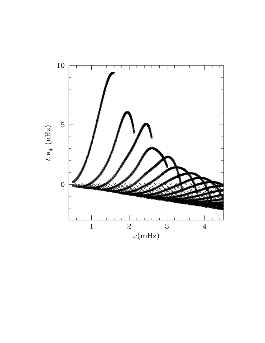
Figure 5: The splitting coefficients $a_{2}$ and $a_{4}$ from effects of rotation.

Figure 6: The splitting coefficients $a_{2}$ and $a_{4}$ plotted as a function of the lower turning point for the modes. The coefficients from GONG and MDI data are compared with the contribution from rotation. Each point represents an average over 30 neighbouring modes.

3.4 Splitting due to magnetic field near the base of the convection zone

There have been some suggestions that a significant toroidal magnetic field may be concentrated in a layer around the base of the convection zone (Dziembowski & Goode 1992). We therefore first investigate splittings that are expected from such a field by assuming the magnetic field to be given by Eq. 16 with

$$a(r)=\cases{\sqrt{8\pi p_{0}\beta_{0}}(1-({r-r_{0}\over d})^{2})&if $|r-r_{0}|\leq d$\cr 0&otherwise\cr}$$ (27)

where $p_{0}$ is the gas pressure, $\beta_{0}$ is a constant giving the ratio of magnetic to gas pressure, $r_{0}$ and $d$ are constants defining the mean position and thickness of layer where the field is concentrated. Fig. 7 shows the splitting coefficients resulting from a toroidal magnetic field of this form concentrated at the base of the convection zone ($r_{0}=0.713R_{\odot}$ and $d=0.02R_{\odot}$). The splitting shown in this and subsequent figures includes both the direct and distortion contributions as defined by Gough and Thompson (1990).

Figure 7: The splitting coefficients $a_{2}$ and $a_{4}$ from a toroidal magnetic field concentrated near the base of the convection zone, plotted as a function of the lower turning point for the mode. Magnetic field is given by Eqs. (16,27) with $k=2$, $\beta_{0}=10^{-4}$, $r_{0}=0.713R_{\odot}$ (shown by the vertical line in the figure) and $d=0.02R_{\odot}$.

The coefficients $a_{2}$ and $a_{4}$ from a toroidal magnetic field concentrated near the base of the convection zone have a characteristic signature for modes with turning point near the base of the convection zone; it should be possible to detect such a signal in the observed splittings if a strong enough magnetic field is indeed present in these layers. The computed splittings, particularly for the deeply penetrating modes in Fig. 7 show a great spread, which is characteristic of the splittings arising from a thin magnetic layer. We return below to the use that can potentially be made of this signature. In the present study, however, we choose to average over neighbouring modes, as discussed in Section 3.3, which suppresses this spread. Our rationale is that the errors in the real data are too large for the spread to be visibly distinguished from noise in the measured splittings at present. Thus we take averages over neighbouring modes and compare the residual after removing the contribution due to rotation with the expected splitting from the magnetic field and the results are shown in Fig. 8. Note that even after averaging a clear signature of the magnetic field is seen in the splitting coefficients. Since we are comparing the average over the same set of modes for the observed splittings and computed splittings for magnetic field, we should be able to get some estimate of magnetic field if a strong enough field does indeed exist. From Fig. 8 it can be seen that there is no clear signature of any feature near the base of the convection zone in the observed splittings, and hence we can only set an upper limit on the magnetic field in this layer. This will of course, depend on the thickness of the magnetic layer. Since there is no clear signature of any signal near the base of the convection zone, for quantitative purpose we take the difference between the lowest and highest point in the range $0.6<r_{t}/R_{\odot}<0.8$ in observed splitting coefficients. For $a_{2}$ this difference is 8.7 nHz for MDI and 7.0 nHz for GONG data, while computed splittings with $\beta_{0}=10^{-4}$ show a difference of 12.6 nHz for a half-thickness of $0.02R_{\odot}$. Thus, we can put an upper limit of $0.7\times 10^{-4}$ on $\beta_{0}$ which corresponds to a magnetic field strength of 300 kG for a layer of half-thickness $0.02R_{\odot}$ near the base of the convection zone. Similar analysis for splitting coefficient $a_{4}$ yields a slightly larger upper limit of 400 kG. These limiting values are close to what was obtained by Basu (1997) using a similar technique and is also consistent with the value independently inferred by D’Silva & Choudhuri (1993). Note, this limit roughly increases as $1/\sqrt{d}$, and clearly, if the thickness of this region is smaller, the upper limit would be larger. It should be noted that the tachocline, where the rotation rate undergoes a transition from differential rotation in the convection zone to a solid-body like rotation in the radiative interior may have a thickness as small as $0.01R_{\odot}$ (Basu 1997; Antia, Basu & Chitre 1998). With this thickness the upper limit on magnetic field would naturally be increased.

Figure 8: The splitting coefficients $a_{2}$ and $a_{4}$ from a toroidal magnetic field concentrated near the base of the convection zone, plotted as a function of the lower turning point of the modes. Each point represents an average over 30 neighbouring modes. The estimated contribution from rotation has been subtracted from the observed splittings plotted in the figure. Magnetic field is given by Eqs. (16,27) with $k=2$, $\beta_{0}=10^{-4}$, $r_{0}=0.713R_{\odot}$ and $d=0.02R_{\odot}$.

Figure 9: The splitting coefficient $a_{2}$ from a toroidal magnetic field concentrated near the base of the convection zone, plotted as a function of the frequency for modes with $\ell\leq 10$. Magnetic field is given by Eqs. (16,27) with $k=2$, $\beta_{0}=10^{-4}$, $r_{0}=0.713R_{\odot}$ and the value of $d$ as marked in the panels.

Figure 10: The splitting coefficients $a_{2}$ and $a_{4}$ from a toroidal magnetic field concentrated in the upper part of the convection zone, plotted as a function of the lower turning point. The larger symbol near the surface represents the average over all f-modes. The estimated contribution from rotation has been subtracted from the observed splittings plotted in the figure. Magnetic field is given by Eq. 27 with $\beta_{0}=10^{-4}$, and the value of $r_{0},d$ and $k$ as marked in the figure.

There is the possibility of distinguishing seismologically between magnetic layers of different thicknesses by using modes that penetrate well beneath the magnetic layer. A thin layer will induce a signature in the $a_{2}$ and $a_{4}$ coefficients which is periodic in mode frequency (Gough & Thompson 1988; Vorontsov 1988; Thompson 1988), in much the same way that the rather sharp transition near the base of the convective envelope produces a periodic signature in the mean frequencies (e.g., Gough 1990; Basu, Antia & Narasimha 1994; Monteiro, Christensen-Dalsgaard & Thompson 1994). Indeed it is this signature which is largely responsible for the vertical spread of points for modes with turning points at radii $r\la 0.6R$ in Fig. 7. Basu (1997) attempted to use this oscillatory signal to obtain an upper limit on magnetic field near the base of convection zone (see also Gough & Thompson  1988). Fig. 9 shows $\ell a_{2}$ for modes with $\ell\leq 10$ for magnetic field concentrated near the base of the convection zone, with two different values of $d$. It is clear that the amplitude of oscillatory signal varies significantly with $d$. However, the observed splitting coefficients for low values of $\ell$ have large errors and it is difficult to extract the small oscillatory signal from these.

3.5 Field in the upper convection zone

Having considered a magnetic field at the base of the convection zone, where theory suggests a field might be stored, we consider where else the data might indicate the presence of magnetic field. There is no signature for the presence of significant magnetic field in the radiative interior, since the averaged residual splitting after correcting for rotation seem to be consistent with zero. However, within the convection zone there is some significant residual splitting, which could be due to the effect of a magnetic field. An inspection of these residuals indicates the existence of a peak around $r=0.96R_{\odot}$, and indeed, if it is due solely to magnetic field, the field may be distributed around this depth ($\approx 28000$ km). It may be noted that this is approximately the depth to which shear layer seen in rotation profile extends (Antia, Basu & Chitre 1998; Schou et al. 1998).

We now attempt to estimate splittings due to the field concentrated in this region. Fig. 10 shows the splittings due to a few magnetic field configurations which are concentrated in the upper part of the convection zone. A comparison of these with the observed splittings indicates that there may be an azimuthal magnetic field with $\beta<10^{-4}$ (i.e., $B\approx 20000$ G), with peak around $r=0.96R_{\odot}$.

The possible existence of a magnetized layer with field of order 20 kG located around $r=0.96R_{\odot}$ is, indeed, a significant inference drawn from our analysis. The physical interpretation for the origin of such a moderately strong magnetic field at this depth below the Sun’s surface is naturally a challenging task for theories of solar dynamo to accommodate. It may be useful to recall here that the numerical simulations of the Sun’s outer convection zone (Nordlund 1999) indicate a major presence of downward moving plumes. It is conceivable that these downdrafts could gather the turbulent magnetic field in the sub-surface layers and carry them to depths in the convective envelope until some sort of equipartition is reached. Interestingly, the density, $\rho$ at a depth of 25–30 Mm is upwards of $4\times 10^{-3}$ gm cm^-3, while the downward velocity for the plumes is of order 500 m s^-1. The dynamical pressure of the plumes, $\rho v^{2}\ga 10^{7}$ dyne cm^-2, then becomes comparable with the magnetic pressure, $B^{2}/8\pi$, corresponding to a field strength of 20–30 kG. It is, therefore, tempting to envisage the formation of such a magnetized layer by the pounding of the downdrafts which tend to concentrate the field at depths where the equipartition of the kind outlined above is approached.

In this study we have assumed a smooth toroidal magnetic field, but in practice we do not expect such a field inside the convection zone. Turbulence may be expected to randomize the magnetic field and such a field may not be expected to produce any significant distortion in the equilibrium state. The direct effect of magnetic field will still be felt though the contribution would be different. Thus our results may be treated as indicating the order of magnitude of field that may be expected if the observed splitting coefficients are indeed due to the magnetic field. If the field is concentrated in flux tubes which occupy only a small fraction of the volume then the required magnetic field could be correspondingly larger. If we assume that the flux tubes occupy a fraction $f$ of the total volume, the magnetic field strength should increase by $1/\sqrt{f}$. If we consider only direct contribution to the splittings then it turns out that $a_{2}$ is always negative for all toroidal field configurations that we tried and hence such a contribution is not likely to explain the observed splittings. But a different magnetic field configuration, e.g., poloidal field might produce $a_{2}$ with the required sign using only direct contribution. The order-of-magnitude splitting caused by a magnetic field is $\ell a_{2}/\nu\sim\beta_{0}\sim v_{A}^{2}/c_{s}^{2}$, where $v_{A}$ is the Alfvén speed. We therefore regard it as unlikely that a different magnetic field configuration would produce a markedly different answer for the field strength required to account for the observed signal in $a_{2}$ and $a_{4}$.

A nonmagnetic latitudinally-dependent perturbation to the wave propagation speed might be responsible for the signal we detect (cf., Gough & Zweibel 1995). Once again we may expect a perturbation of order $10^{-4}$ located in the region around $r=0.96R_{\odot}$ to yield the observed splittings. Gough et al. (1996) inferred a perturbation of that magnitude, of unspecified origin, from earlier GONG data. A temperature variation of order 10K, suitably confined, might conceivably produce a similar signature. In fact, Kuhn (e.g., Kuhn 1996) has argued that the thermal shadow of belts of magnetic flux near the bottom of the convection zone can have a significant effect on the even a-coefficients. But Kuhn’s models show the largest temperature perturbations occurring in the very superficial superadiabatic layer, at a depth of a small fraction of one per cent of the solar radius. Such a perturbation alone would be consistent with the f-modes having a small residual splitting, but would not explain the apparent overturning of the p-mode splittings at $r_{t}\approx 0.96R$. A magnetic field at some depth below the surface may explain both aspects. We certainly do not rule out the possibility that some nonmagnetic asphericity, which we have not considered in detail in this study, may account for some of the observed splittings.

4 Conclusions

Second order correction to mean frequencies due to rotation is comparable to the error estimates in the observed frequencies. The error in helioseismic inversion introduced by the frequency shift due to rotation is $\la 10^{-4}$, which is much smaller than the estimated errors in inversions. Further, a part of this frequency shift is expected to be nullified by the general relativistic effects. The shift in f-mode frequencies due to rotation can reduce the estimated solar radius by 4 km. The distortion due to rotation can yield surface oblateness of $-5.8\times 10^{-6}$ and $6.2\times 10^{-7}$ in the $P_{2}(\cos\theta)$ and $P_{4}(\cos\theta)$ components, respectively. This is in reasonable agreement with observed oblateness at the solar surface (Kuhn et al. 1998) and it appears that most of the observed distortion is accounted by the seismically inferred rotation rate in solar interior. The quadrupole moment $J_{2}=-2.18\times 10^{-7}$ resulting from rotational distortion is small enough to maintain consistency of the general theory of relativity.

After subtracting the estimated contribution from rotation to the splitting coefficients $a_{2}$ and $a_{4}$ from the observed splittings, there is a small residual which is statistically significant in the convection zone. This could arise from a magnetic field. From the magnitude of residual in observed splittings we can tentatively conclude that magnetic field with $\beta\approx 10^{-4}$ may be present in the upper part of the convection zone. This corresponds to an azimuthal magnetic field of $\approx 20$ kG around $r=0.96R_{\odot}$. However, we cannot rule out the possibility that this signal in splitting coefficients may arise from some aspherical perturbation to the temperature field. This would be practically indistinguishable from the effect of a magnetic field using just the mode frequencies (Gough & Zweibel 1995); but complementary analyses such as time-distance helioseismology might be able to distinguish them, since the local direct effect of a magnetic field on the waves is anisotropic, whereas that of a temperature perturbation is not.

A toroidal magnetic field that is concentrated near the base of the convection zone gives a characteristic pattern in the splittings for modes with lower turning point in that region. Since no such signal is seen in observed frequencies, we can put an upper limit of about 300 kG on the strength of the magnetic field in this region.

- (1) Antia H. M. 1996, A&A 307, 609
- (2) Antia H. M. 1998, A&A 330, 336
- (3) Antia H. M., Basu S., Chitre S. M. 1998, MNRAS 298, 543
- (4) Armstrong J., Kuhn J. R. 1999, ApJ 525, 533
- (5) Basu S. 1997, MNRAS 288, 572
- (6) Basu S., Antia H. M., Narasimha D. 1994, MNRAS 267, 209
- (7) D’Silva S., Choudhuri A. R. 1993, A&A 272, 621
- (8) Dziembowski W. A., Goode P. R. 1992, ApJ 394, 670
- (9) Dziembowski W. A., Goode P. R., DiMauro M. P., Kosovichev A. G., Schou J. 1998, ApJ 509, 456
- (10) Gough D. O. 1990, in Progress of seismology of the sun and stars, eds. Y. Osaki & H. Shibahashi, Lecture Notes in Physics, 367, Springer, Berlin, p283
- (11) Gough D. O., Thompson M. J. 1988, in Advances in helio- and asteroseismology, Proc. IAU Symp. 123, Eds. J. Christensen-Dalsgaard & S. Frandsen, D. Reidel, Dordrecht, p155
- (12) Gough D. O., Thompson M. J. 1990, MNRAS 242, 25
- (13) Gough D. O., Zweibel E. G. 1995, in Proc. 4th SOHO workshop, eds. J. T. Hoeksema, V. Domingo, B. Fleck, B. Battrick, ESA SP-376, ESTEC, Noordwijk, p73
- (14) Gough D. O., Kosovichev A. G., Toomre J., et al. 1996, Sci. 272, 1296
- (15) Hill F., Stark P. B., Stebbins R. T., et al. 1996, Sci. 272, 1292
- (16) Howe R., Komm R., Hill F. 1999, ApJ 524, 1084
- (17) Kuhn J. R. 1996, in The Structure of the Sun, VI Canary Islands Winter School of Astrophysics, Cambridge Univ. Press, Eds. T. Roca Cortès & F. Sánchez, p231
- (18) Kuhn J. R., Bush R. I., Schelck X., Scherrer P. 1998, Nature 392, 155
- (19) Libbrecht K. G., Woodard M. F. 1990, Nature 345, 779
- (20) Monteiro M. J. P. F. G., Christensen-Dalsgaard J., Thompson M. J. 1994, A&A 283, 247
- (21) Nordlund Å 1999, IAU Colloquium 179 on Cyclical evolution of solar magnetic fields: Advances in theory and observations
- (22) Pijpers F. P. 1998, MNRAS 297, L76
- (23) Rhodes E. J., Kosovichev A. G., Schou J., Scherrer P. H., Reiter J. 1997, Solar Phys. 175, 287
- (24) Ritzwoller M. H., Lavely E. M. 1991, ApJ 369, 557
- (25) Schou J., Christensen-Dalsgaard J., Thompson M. J. 1994, ApJ 433, 389
- (26) Schou J., Kosovichev A. G., Goode P. R., Dziembowski W. A. 1997, ApJ 489, L197
- (27) Schou J., Antia H. M., Basu S., et al. 1998, ApJ 505, 390
- (28) Thompson M. J. 1988, in Seismology of the Sun & Sun-like Stars, Eds. V. Domingo & E. J. Rolfe, ESA SP-286, p321
- (29) Thompson M. J., Toomre J., Anderson E. R., et al. 1996, Sci. 272, 1300
- (30) Tripathy S. C., Antia H. M. 1999, Solar Phys. 186, 1
- (31) Vorontsov S. V. 1988, in Advances in helio- and asteroseismology, Proc. IAU Symp. 123, Eds. J. Christensen-Dalsgaard & S. Frandsen, D. Reidel, Dordrecht, p151