A disk-wind model with correct crossing of all MHD critical surfaces

Abstract

The classical Blandford & Payne (1982) model for the magnetocentrifugal acceleration and collimation of a disk-wind is revisited and refined. In the original model, the gas is cold and the solution is everywhere subfast magnetosonic. In the present model the plasma has a finite temperature and the self-consistent solution of the MHD equations starts with a subslow magnetosonic speed which subsequently crosses all critical points, at the slow magnetosonic, Alfvén and fast magnetosonic separatrix surfaces. The superfast magnetosonic solution thus satisfies MHD causality. Downstream of the fast magnetosonic critical point the poloidal streamlines overfocus towards the axis and the solution is terminated. The validity of the model to disk winds associated with young stellar objects is briefly discussed.

1 Introduction

Astrophysical jets are systematically associated with the presence of an underlying accretion disk, both observationally and theoretically (see Königl & Pudritz 2000 for a recent review). In the case of protostellar objects, accretion disks are resolved by means of infrared and millimeter surveys and interferometric mappings down to scales of a few tens of AU. In the optical and the near infrared, HST high resolution images of disks in several jet sources have also been obtained (Padgett et al. 1999). With an apparent relation found between accretion and ejection in the form of a strong correlation between outflow signatures and accretion diagnostics (see e.g. Cabrit et al. 1990, Cabrit & André 1991, Hartigan et al. 1995), stellar jets seem to be powered by the gravitational energy released in the accretion process.

These facts and considerations have led several authors to develop models of disk winds. The pioneering work of Bardeen & Berger (1978) on a hydrodynamic radially self-similar model of a hot galactic wind was generalized in the seminal paper of Blandford & Payne (1982, henceforth BP82) by including a rotating magnetic field. In particular, in BP82 it was shown that a cold plasma can be launched magneto-centrifugally from a Keplerian disk, similarly to a bead on a wire, provided that the magnetic field lines are sufficiently inclined from the axis. Since then, steady and axisymmetric MHD models, self-similar in the radial direction, have been successfully analyzed and generalized in the literature (see e.g. Contopoulos & Lovelace 1994, henceforth CL94, Li 1995, 1996, Ferreira 1997, Ostriker 1997, Vlahakis & Tsinganos 1998, henceforth VT98, Lery et al. 1999).

A major problem is however still open on the validity of the various classes of radially self-similar solutions analyzed so far. Because, as it is well known since the original work of Weber & Davis (1967) on the rotating magnetized solar wind in the equatorial region, acceptable outflowing solutions must cross smoothly all singularities related to the characteristic speeds of the MHD perturbations, i.e., the poloidal Alfvén velocity and the slow/fast magnetosonic velocities. However, in radially self-similar equations the critical points are not found where the poloidal speed of the flow is equal to the characteristic velocities of these magnetosonic waves. In the cold model of BP82 the “modified” fast magnetosonic critical point (where $t=1$ in the BP82 notation) is found downstream of the position where the poloidal velocity of the wind is equal to the fast magnetosonic velocity. Subsequently it has been shown that this is a general property of the axisymmetric steady MHD equations: the singularities of the equations coincide with the positions of the limiting characteristics, or separatrices, within the hyperbolic domain of the governing equations (Bogovalov 1994, Tsinganos et al. 1996). In particular, Bogovalov (1994, 1996) pointed out the key role played by the singularity occurring at the fast magnetosonic separatrix surface (FMSS). Namely, the asymptotic region of the jet is causally disconnected from the base of the flow, only for solutions that cross the critical point at the FMSS. This means that every terminal perturbation or shock does not affect the outflow structure upstream of the position of this critical point. And, Tsinganos et al. (1996) have given several analytical examples where the true singularities of the equations do not coincide with the positions where the governing partial differential MHD equations change character from elliptic to hyperbolic and vice versa. For the sake of simplicity from now on we shall indicate by ‘fast/slow magnetosonic singularity’, or in short ’modified fast/slow’, the critical points at the FMSS/SMSS.

It turns out that in none of the previous models of disk-winds a solution has been found to cross the FMSS. For example, Li (1995, 1996) and Ferreira (1997), starting from the accretion disk, succeeded to cross the slow magnetosonic and the Alfvén ones, but downwind turning points were found where the solutions terminate. Such solutions can be connected to infinity only through a shock, as suggested by Gomez de Castro & Pudritz (1993). However in this case, as the wind velocity is subfast magnetosonic, a temporal evolution of the outflow is expected (Ouyed & Pudritz 1997).

Cylindrically collimated solutions were found by Ostriker (1997) for a cold plasma, integrating the MHD system upstream from infinity and crossing the Alfvén singularity, but always in the subfast magnetosonic regime. On the other hand, it has been shown that in collimated winds oscillations of streamlines are a common feature (Vlahakis & Tsinganos 1997). It thus seems that cylindrically collimated solutions without oscillations correspond to a rather particular choice of parameters that completely suppresses such oscillations. A slight change in these parameters induces the onset of oscillations which increase in amplitude until the configuration is destroyed (Vlahakis 1998). Since the Ostriker (1997) solutions are asymptotically subfast magnetosonic they are likely to be sensitive to perturbations from the external medium, unlike solutions that really satisfy all the criticality conditions. Therefore, such solutions are likely to be structurally and topologically unstable (Vlahakis 1998).

However, it has been shown by Contopoulos (1995) that, in the restricted case of a purely toroidal magnetic field, a smooth crossing of the FMSS is possible. On the other hand in such a case an asymptotically cylindrically collimated configuration is not found; in fact, a new transition to subfast magnetosonic velocities must occur anyway for radially self-similar winds. The only way out is then to match the superfast magnetosonic solution with a shock which is in this case in the physically disconnected domain.

In the present study we extend the analysis of BP82, CL94 and Contopoulos (1995) showing that an exact and simultaneous smooth crossing of all three MHD critical surfaces is possible. In Sec. 2 we define the equations of the hot wind in the framework of a radially self-similar approach and outline the numerical technique. In Sec. 3 we explore the solution topologies in the region around and particularly downstream of the FMSS, where the solution terminates, while in Sec. 4 are shown the features of a few solutions crossing all three critical points with conditions similar to those of BP82. Finally, in Sec. 5 we discuss the possible astrophysical applications of these solutions to stellar jets, and summarize the main implications of our results in comparison with previous ones obtained by other authors.

2 Model description

In order to establish notation, in this Section we give a brief derivation of radially self-similar disk-wind models with polytropic thermodynamics. The derivation is along the lines of a systematic method which unifies all self-similar MHD outflows and includes the BP82 model as the simplest case (VT98).

2.1 General definitions and self-similar assumption

In steady $(\partial t=0)$ and axisymmetric $(\partial\phi=0)$ MHD, the poloidal components of the hydromagnetic field ($\hbox{\bf B},\hbox{\bf V}$) are defined in terms of the magnetic flux function $A$ and mass to magnetic flux function $\Psi_{A}(A)$ in cylindrical ($z\,,\varpi\,,\phi$) or spherical ($r\,,\theta\,,\phi$) coordinates, as:

$$\hbox{\bf B}_{p}=\nabla\times\frac{A\hat{\phi}}{\varpi}\,,\qquad\hbox{\bf V}_{p}=\frac{\Psi_{A}(A)}{4\pi\rho}\hbox{\bf B}_{p}\,.$$ (1)

The azimuthal components are defined in terms of the total specific angular momentum $L(A)$ and of the corotation frequency $\Omega(A)$, which are functions of $A$ (Tsinganos 1982):

$$L(A)=\varpi\left(V_{\phi}-\frac{B_{\phi}}{\Psi_{A}}\right)\,,\;\;\;\Omega(A)=\frac{1}{\varpi}\left(V_{\phi}-M^{2}\frac{B_{\phi}}{\Psi_{A}}\right)\,,$$ (2)

and of the poloidal Alfvén number $M$ :

$$M=\sqrt{4\pi\rho}\frac{V_{p}}{B_{p}}=\frac{\Psi_{A}}{\sqrt{4\pi\rho}}\,.$$ (3)

TransAlfvénic flows require that, when $M=1$, $V_{\phi}$ and $B_{\phi}$ are finite, i.e.:

$${L\over\Omega}=\varpi_{\alpha}^{2}(A)\equiv\varpi_{\star}^{2}\alpha\,,$$ (4)

where $\varpi_{\star}$ is the Alfvén cylindrical radius (the Alfvén lever arm) along the reference field line $\alpha=1$, with the dimensionless variable $\alpha$ defined as some function of the magnetic flux function $A$ which can be reversed to give:

$$A=\frac{B_{\star}\varpi_{\star}^{2}}{2}{\cal A}\left(\alpha\right)\,.$$ (5)

where $B_{\star}$ is a constant with the dimensions of a magnetic field.

As shown in VT98, all existing classes of radially self-similar MHD solutions can be constructed by making the following two key assumptions:
(i) the Alfvén number $M$ is solely a function of $\theta$, such that the Alfvén surface is conical:

$$M\equiv M(\theta)\,,$$ (6)

(ii) the cylindrical distance $\varpi$ to the polar axis of some fieldline labeled by $\alpha$, normalized to its cylindrical distance $\varpi_{\alpha}$ at the Alfvén point is also solely a function of $\theta$:

$$G\left(\theta\right)\equiv\frac{\varpi}{\varpi_{\alpha}}\,.$$ (7)

Following these two assumptions the set of MHD equations is reduced to a system of three ordinary differential equations in $\theta$ for $M(\theta)$, $G(\theta)$ and the $\theta$ -dependence of the gas pressure (see VT98 for details).

2.2 Polytropic thermodynamics

Depending on the assumptions on the free integrals $A(\alpha)$, $\Psi_{A}(\alpha)$, $L(\alpha)$ and $\Omega(\alpha)$, a few classes of radially self-similar solutions exist (see VT98). For only two of these classes a polytropic relationship between the gas pressure and the density is admitted: $P=Q(\alpha)\rho^{\gamma}$, where $Q(\alpha)$ is the specific entropy (the first two cases listed in Table 3 of VT98). In such a case $A\propto\alpha^{x/2}$, $\Psi_{A}\propto\alpha^{(x-3/2)/2}$, $\Omega\propto\alpha^{-3/4}$, $L\propto\alpha^{1/4}$, and the system of the MHD equations reduces to two first order differential equations for $M(\theta)$ and $G(\theta)$, supplemented by the Bernoulli integral which also provides the variable $\psi(\theta)$, the angle between a particular poloidal fieldline and the cylindrical direction $\hat{\varpi}$ at the spherical angle $\theta$. Note that the parameter $x$ (with the same notation as in CL94, while in VT98 $x$ was denoted by $F$) governs the scaling of the magnetic field, while the rotation law is assumed Keplerian. This particular class corresponds to the radially self-similar solutions analyzed in CL94 which contains as a special case the classical BP82 solution with $x=0.75$.

The full expressions of ${\rm d}M^{2}/{\rm d}\theta$, ${\rm d}G^{2}/{\rm d}\theta$ and $\psi(\theta$) are given in the Appendix, Eqs. (A1) - (A3) The expressions for the physical variables become then:

$$\frac{\rho}{\rho_{\star}}=\alpha^{x-3/2}\frac{1}{M^{2}}\,,\qquad\frac{P}{P_{\star}}=\alpha^{x-2-\gamma\left(x-3/2\right)}\left(\displaystyle\frac{\rho}{\rho_{\star}}\right)^{\gamma}\,,$$ (8)

$$\frac{\hbox{\bf B}_{p}}{B_{\star}}=-\alpha^{\frac{x}{2}-1}\frac{1}{G^{2}}\displaystyle\frac{\sin\theta}{\cos\left(\psi+\theta\right)}\left(\sin\psi\hat{z}+\cos\psi\hat{\varpi}\right)\,,$$

$$\frac{\hbox{\bf V}_{p}}{V_{\star}}=-\alpha^{-1/4}\frac{M^{2}}{G^{2}}\displaystyle\frac{\sin\theta}{\cos\left(\psi+\theta\right)}\left(\sin\psi\hat{z}+\cos\psi\hat{\varpi}\right)\,,$$

$$\frac{B_{\phi}}{B_{\star}}=-\lambda{\alpha}^{\frac{x}{2}-1}\displaystyle\frac{1-G^{2}}{G\left(1-M^{2}\right)}\,,$$ (9)

$$\frac{V_{\phi}}{V_{\star}}=\lambda{\alpha}^{-1/4}\displaystyle\frac{G^{2}-M^{2}}{G\left(1-M^{2}\right)}\,.$$ (10)

2.3 Parameters

At the Alfvén radius $\varpi_{\star}$ along the reference field line $\alpha=1$, we denote by $P_{\star}$ and $\rho_{\star}$ the pressure and density, respectively. The magnitude of the poloidal magnetic field at this Alfvén point is $-B_{\star}\,{\sin\theta_{\star}}/{\cos\left(\psi_{\star}+\theta_{\star}\right)}$ while the corresponding poloidal Alfvén speed is $-V_{\star}\,{\sin\theta_{\star}}/{\cos\left(\psi_{\star}+\theta_{\star}\right)}$, with $B_{\star}=\sqrt{4\pi\rho_{\star}}V_{\star}$.

The expressions of the free integrals defined in Sec. 2.1 can now be written as:

$$A=\displaystyle\frac{B_{\star}\varpi_{\star}^{2}}{x}\alpha^{x/2}\,,\qquad\Psi_{A}^{2}=\displaystyle 4\pi\rho_{\star}\alpha^{x-3/2}\,,$$ (11)

$$\Omega=\displaystyle\lambda\frac{V_{\star}}{\varpi_{\star}}\alpha^{-{3/4}}\,,\qquad L=\lambda V_{\star}\varpi_{\star}\alpha^{{1/4}}\,,$$ (12)

$$E=V^{2}_{\star}\epsilon\alpha^{-1/2}\,,\qquad V^{2}_{\star}=\displaystyle\frac{{\cal G}{\cal M}}{{\varpi_{\star}}\kappa^{2}}\,,\qquad P_{\star}=\displaystyle\mu\frac{B^{2}_{\star}}{8\pi}\,,$$ (13)

where $E$ is the sum of the kinetic, enthalpy, gravitational and Poynting energy flux densities per unit of mass flux density,

$$E(\alpha)=\frac{V^{2}}{2}+\frac{\gamma}{\gamma-1}\frac{P}{\rho}-\frac{{\cal G}{\cal M}}{r}-\frac{\Omega}{\Psi_{A}}r\sin\theta B_{\phi}\,,$$ (14)

while ${\cal G}$ and ${\cal M}$ are the gravitational constant and the mass of the central body, respectively.

The solution of the system of Eqs. (A1) - (A3) depends on the six parameters $x$, $\gamma$, $\kappa$, $\lambda$, $\epsilon$ and $\mu$, introduced in Eqs. (11) - (13) (but see the discussion in Sect. 2.4.3 for the free parameters of the model). Note that we have used for the parameters a similar but not an identical notation with BP82, since it occurred to us that it is better to choose a different normalization. However, in the following we shall outline for convenience the correspondence between our parameters and those in BP82.

Let us first discuss the physical meaning of the above parameters. First, the exponent $x$ is equal to $3/4$ in BP82, while in Ferreira (1997) it is related to the ejection index $\xi=2(x-3/4)$. This index $\xi$ is related to the accretion rate and to the mass flux in the wind if also the structure of the disk is assumed radially self-similar (see e.g. Ferreira 1997). Second, we remind that $\gamma$ is the usual polytropic index. Next, the constant $\kappa$ is the Keplerian speed at radius $\varpi_{\star}$ on the disk, in units of $V_{\star}$, i.e., it is proportional to the ratio of the Keplerian speed to the poloidal flow speed at the Alfvén radial distance, $V_{\rm p,A}$, and is related to the corresponding constant $\kappa_{\rm BP}$ in BP82. Since $\kappa$ is also proportional to the mass to magnetic flux ratio, it is often called ’the mass loss parameter’ (Li 1995, Ferreira 1997),

$$\kappa=\sqrt{\frac{{\cal G}{\cal M}}{\varpi_{\star}V_{\star}^{2}}}=-\sqrt{\frac{{\cal G}{\cal M}}{\varpi_{\star}V^{2}_{\rm p,A}}}\frac{\sin\theta_{\star}}{\cos\left(\psi_{\star}+\theta_{\star}\right)}=\kappa_{\rm BP}G^{-3/2}_{o}\,.$$ (15)

The constant $\lambda$ is the specific angular momentum of the flow in units of $V_{\star}\varpi_{\star}$ and is related to the corresponding constant $\lambda_{\rm BP}$ in BP82,

$$\lambda=\frac{L}{V_{\star}\varpi_{\star}}=\lambda_{\rm BP}\kappa\sqrt{G_{o}}\,.$$ (16)

The Bernoulli constant $\epsilon$ is the sum of the enthalpy, kinetic, gravitational and Poynting energy flux densities per unit of mass flux density divided by $V_{\star}^{2}$ (along $\alpha=1$) and is related to the corresponding constant $\epsilon_{\rm BP}$ in BP82,

$$\epsilon=\frac{E}{V_{\star}^{2}}=\epsilon_{\rm BP}\frac{\kappa^{2}}{G_{o}}\,.$$ (17)

Finally, the constant $\mu$ is proportional to the gas entropy,

$$\mu=\mu_{\rm BP}\left[2G_{o}^{3\gamma-4}\sin^{2\gamma-2}\psi_{o}\kappa^{2\gamma}\right]\,.$$ (18)

In the above expressions, the label $o$ indicates the respective values of $G$ and $\psi$ at the base of the outflow. The correspondence between the parameter $\xi^{\prime}_{o}$ in BP82 and our $\psi_{o}$ is

$$\xi^{\prime}_{o}=\cot\psi_{o}\,.$$ (19)

Note that in BP82 $\gamma$ does not appear since the outflow is cold and $\mu$, although it is defined, is never used. Also, a similar scaling exists for the parameters used in Li (1995) and Ferreira (1997), although with slightly different notations and a further relation between $x$ and $\kappa$ (cf. Eq. 28 in Ferreira 1997) due to the connection with a self-similar accretion disk thread by a large scale magnetic field.

2.4 Numerical integration

The numerical solution of Eqs. (A1)-(A3) requires the fulfillment of the regularity conditions at the positions of the three singularities (Alfvén and slow/fast modified magnetosonic critical points). This implies that the six parameters of the solution are not all independent. In the following we first shortly summarize the main properties of the critical conditions before we discuss the numerical procedure to obtain the solutions.

2.4.1 Critical Points

It is evident that Eqs. (A2) and (A3) become indeterminate at the Alfvén surface where $G=M=1$. The regularity condition at this critical point can be easily found together with the value of the derivative of $M^{2}$ (see Appendix). Furthermore, the denominator of Eq. (A2) vanishes when the meridional component of the velocity $V_{\theta}$ satisfies the quartic (Vlahakis 1998):

$$V_{\theta}^{4}-V_{\theta}^{2}\left(C_{s}^{2}+V_{A}^{2}\right)+C_{s}^{2}V^{2}_{A\,,\theta}=0\,,$$ (20)

where $C_{s}$ is the sound speed, and $V_{A}$ and $V_{A\,,\theta}$ the total and meridional components of the Alfvén velocity, respectively.

These singularities are typical ‘X-type’ critical points, and the above equation is the well known dispersion relation for the magnetosonic waves. However it is crucial to see that these singularities appear not when the flow speed, but instead where its meridional component coincides with the meridional component of the slow/fast magnetosonic velocity.

Bogovalov (1994, 1996) and Tsinganos et al. (1996) have emphasized that the singularities in MHD steady flows do not always coincide with the positions where the flow and the magnetosonic velocities coincide, but with the limiting characteristics, i.e., the FMSS and the SMSS. In our case the separatrix is found where $V_{\theta}$ is equal to either one of the triplet of the characteristic speeds ($V_{s,\theta},V_{A,\theta},V_{f,\theta}$). This is so because in addition to the azimuthal direction $\hat{\phi}$ due to the assumed axisymmetry, we have a second symmetry direction, which is the radial direction $\hat{r}$ because of the assumed radial self-similarity. Therefore a compressible slow/fast MHD wave that preserves those two symmetries can only propagate along $\hat{\theta}$ which is perpendicular to both $\hat{\phi}$ and $\hat{r}$; the speed of propagation of such a wave satisfies exactly the quartic Eq. (20) (for details see Tsinganos et al. 1996).

It is obvious that a physically acceptable solution with low velocity and high density at the base, but high speed and low density asymptotically must smoothly cross at least the SMSS and the Alfvén singularity. Such solutions have been widely analyzed in previous papers and are consistent with the observational data on collimated stellar jets. However it is unescapable that also the fast magnetosonic singularity should be regularly crossed in order to have a steady structure causally disconnected from the asymptotic region, where the jet interacts with the environment (Bogovalov 1994).

2.4.2 Numerical technique for the search of solutions

An inherent difficulty of the problem is due to the fact that the positions of the previous critical points are not known a-priori, but need to be calculated simultaneously and selfconsistently with the sought for solution. At these critical points we do know some relations between various functions, for example, at the Alfvén surface the regularity condition, Eq. (A4), should be satisfied. However, this knowledge alone is not practically enabling us to directly find a solution.

The way we will follow to construct a solution through all critical points is to use the shooting method with successive iterations. By starting the integration from an angle $\theta=\theta_{i}$ we reach a singular point where, e.g., the denominator in $dM^{2}/d\theta$ vanishes, but not the numerator. We then go back and change some parameter and integrate again until it converges, i.e., the denominator and the numerator vanish simultaneously. A similar procedure is followed to cross the other singularity. A rather key point is the choice of the starting position of integration. Most of the previous studies solved the equations by starting from the equator (BP82, CL94), or from infinity (Ostriker 1997). It occurred to us that it is more convenient to integrate the equations starting from the Alfvén critical point, i.e. from the conical surface $\theta=\theta_{\star}$, and move upstream (towards the base) and downstream (towards the external asymptotic region).

For the numerical integration, besides the parameters, we need also to choose the value of the colatitude $\theta_{\star}$ and the value there of the slope of the square of the Alfvén number ($p_{\star}={{\rm d}M^{2}}/{{\rm d}\theta}|_{\theta_{\star}}$) together with the angle of expansion of the poloidal streamlines ($\psi_{\star}$). Some of these quantities must be tuned to fulfill the singularity conditions at the three critical points. It turned out convenient for the assumed numerical technique to tune the values of $\lambda$ and $p_{\star}$ for getting the critical solution.

Hence, we first prescribe the parameters $\gamma$, $x$, $\lambda$ and $\kappa$, as well as $p_{\star}$, $\theta_{\star}$ and $\psi_{\star}$ while $\epsilon$ is deduced from the Bernoulli equation, Eq. (A3), and $\mu$ from the regularity condition at the Alfvén point, Eq. (A4). The integration can now start upstream from $\theta=\theta_{\star}$ and the SMSS is encountered, but we cannot pass through it as, e.g., the denominator of $dM^{2}/d\theta$ vanishes there, but not the numerator. We integrate again with different values of $p_{\star}$ until we find the opposite behaviour around the slow magnetosonic singularity (the numerator vanishes but not the denominator). Iteratively, by fine tuning the value of $p_{\star}$, a solution is finally found which pass through the SMSS.

Then we integrate downstream of the Alfvén surface and the FMSS is encountered, but in general it is not crossed. Changing the value of the parameter $\lambda$ we integrate upstream again tuning to a new value of $p_{\star}$ until the SMSS is crossed. Then we integrate downstream towards the fast magnetosonic singularity, and repeat all the procedure until we find the right values of $p_{\star}$ and $\lambda$ that allow the crossing of the two singularities. At this point the complete solution is obtained by integrating, with the correct values for all the parameters, upstream to the base and downstream towards the asymptotic region.

2.4.3 Selection of the parameters and boundary conditions

In this study, the critical solution depends on the two ‘model’ parameters ($\gamma$, $x$) and the three independent ‘fieldline’ parameters ($\kappa$, $\theta_{\star}$, $\psi_{\star}$). The remaining ones ($\epsilon$, $\mu$, $p_{\star}$, $\lambda$) are deduced from the Bernoulli equation and the crossing of the Alfvén, slow magnetosonic and fast magnetosonic singularities, respectively. This is consistent with the analysis of Bogovalov (1997) where it is argued that since the number of equations must be equal to the number of independent boundary conditions, a unique solution can be found if this number of independent boundary conditions equals to the number of outgoing waves generated at the reflection of a plane wave from that boundary. In $t$-dependent polytropic MHD there are 7 equations and 7 unknowns: the density, the pressure, the 3 components of the velocity and the 2 components of the magnetic field. There are also 7 waves: the entropy wave and the outwards/inwards propagating slow, Alfvén and fast MHD waves. So, we need 7 parameters with both counts, as expected. Now, if the boundary of the outflow is in the subslow region the number of outgoing waves from this boundary is 4, i.e., the entropy, slow, Alfvén and fast MHD outgoing waves. Subtracting the number of the boundary conditions we are left with 3 independent parameters, precisely $\kappa$, $\theta_{\star}$ and $\psi_{\star}$. Note that the polytropic index $\gamma$ and $x$ should not be included in this count since they are model parameters and do not depend on a particular streamline.

Figure 1: Solution topologies around the FMSS for $\gamma=1.24$ (left) and $\gamma=1.23$ (right). The other parameters are shown in Tab. 1. The critical solution drawn with a solid line crosses the line $M_{\rm m,f}=1$ at $\theta=\theta_{\rm m,f}\approx 6^{\circ}$ while the noncritical topologies are plotted with dashed and dot-dashed lines. For $\theta>\theta_{\rm m,f}$ and $M_{\rm m,f}<1$ the three different branches of the solutions overlap.

The integration is terminated in the upstream region when $M\rightarrow M_{o}<1$ and $G\rightarrow G_{o}<1$, $\theta\rightarrow\theta_{o}\approx\pi/2$ and $\psi=\psi_{o}$. In all the calculations presented here we were able to follow the solution up to the equator, i.e. $\theta_{o}=\pi/2$. This base should be in principle the disk surface, where our solutions should consistently fit particular boundary conditions. Such an approach has been followed by Ferreira (1997) who looked for inflow/outflow MHD solutions with a consistent matching on the disk surface (see also Li 1995, 1996). This implies some further constraints on the parameters. For instance, if the disk is also self-similar with a large scale magnetic field, a relation between $\kappa$ and $x$ is expected, i.e., the mass loading in the outflow and the magnetic flux distribution on the disk. In addition, if the outflow carries away all the angular momentum from the disk $x$ must be related to $\lambda$.

As described above, the procedure to obtain a critical solution is extremely lengthy and rather time consuming. We must in fact approach as close as possible the singularities ($\Delta\theta\approx 10^{-3}$), and this requires the determination of the parameters up to several digits. As we are mainly concerned to analyze the general behaviour of superfast magnetosonic solutions, in the present study we do not investigate the details of the boundaries of the outflow. Therefore we assume that between the base of the wind and the disk surface there is a thin ‘transition’ region that allows the connection of the wind with the disk.

For similar reasons the present analysis has been performed only for a limited set of values of the parameters. We have fixed the ‘fieldline’ parameters $\theta_{\star}=59^{\circ}$, $\psi_{\star}=40^{\circ}$ and $\kappa=2$, while two values have been assumed for the ‘model’ parameter $x$: 0.75 (model I) and 0.7525 (model II). In this two cases we will assume that the polytropic index $\gamma<5/3$, i.e. some amount of heating occurs in the plasma. To make a comparison with a purely magnetocentrifugally driven outflow, we shortly discuss also the very general properties of an adiabatic solution ($\gamma=5/3$) assuming $\theta_{\star}=60^{\circ}$, $\psi_{\star}=45^{\circ}$, $\kappa=3.873$ and $x=0.75$ (i.e., values of $\theta_{\star}$ and $\psi_{\star}$ very close to those used for the nonadiabatic models I and II on purpose have been selected).

In the following two Sections we outline the main properties of the topologies around the FMSS and discuss the structure of the critical solutions.

3 Solution Topologies

We present here the topology of two solutions around the fast magnetosonic point, assuming $\gamma=1.24$ and $\gamma=1.23$ for fixed $x=0.75$. The two slightly different values of the polytropic index define the transition between two families of topologies. This drastic change in the topological behavior of the solutions in the neighborhood of the X-type point illustrates the difficulty of exact crossing the fast magnetosonic point. The parameters for the various cases are listed in Tab. 1, while in Fig. 1 we plot the two sets of topologies for the superfast magnetosonic number $M_{\rm m,f}(\theta)$. Note that this plot is obtained from a projection of the solutions from the 3-D space of $M(\theta)$, $G(\theta)$ and $\theta$ to the plane $M_{\rm m,f}$ – $\theta$. This three-dimensional structure of the topology explains why some of the lines obtained by projection are crossing each other (see for another such example Tsinganos & Sauty 1992). This feature of course does not appear in more classical topologies of one-dimensional solutions, e.g., Weber & Davis (1967).

In the first case ($\gamma=1.24$) three solutions are plotted in Fig. 1a for different values of $\lambda$ and $\mu$. The critical solution (solid line in Fig. 1a), moving downstream in the direction of decreasing $\theta$ crosses the FMSS at $\theta_{\rm m,f}\approx 6^{\circ}$, has a maximum at $\theta\approx 0.4^{\circ}$ and then at $\theta\approx 0.15^{\circ}$ crosses back the $M_{\rm m,f}=1$ line but with an infinite slope moving towards increasing $\theta$. Then, this solution continues marching towards increasing $\theta$ and remains always subfast magnetosonic, with $M_{\rm m,f}$ reaching a maximum at $\theta\approx\theta_{\rm m,f}$.

By slightly decreasing $\lambda$ the solution crosses the $M_{\rm m,f}=1$ line with infinite slope at $\theta>\theta_{\rm m,f}$ (dashed line in Fig. 1a). Conversely, for a slightly larger value of $\lambda$ the solution (dot-dashed line in Fig. 1a) reaches a maximum at $\theta\approx\theta_{\rm m,f}$ remaining subfast magnetosonic (i.e. it behaves like a ‘breeze’ solution) and becomes superfast magnetosonic with diverging slope at $\theta\approx 0.04^{\circ}$. Then, this solution remains always in the region $\theta<\theta_{\rm m,f}$, with a spiraling behaviour, i.e., by crossing many times up and down the $M_{\rm m,f}=1$ transition with infinite slope. Note that the solution shown in Fig. 10 of Ferreira (1997) probably belongs to this family of non critical solutions.

For $\gamma=1.23$ (Fig. 1b) the topology of the non critical solutions remains the same. The critical solution however shows a different behaviour remaining always in the region $\theta<\theta_{\rm m,f}$ by spiraling around the $M_{\rm m,f}=1$ transition (solid line in Fig. 1b).

The topological structure of our solutions implies that downstream of the FMSS a focal critical point must be present, so that no solution can asymptotically reach $\theta=0$ with superfast magnetosonic speeds. This ought to be expected from the construction of this model where we should have $\lim_{\theta\to 0}{V_{\theta}}/{V_{{\rm f},\theta}}=0$, if we have a cylindrically collimated outflow. In other words, the surface $M_{\rm m,f}=1$ needs to be crossed again with a downstream superfast/subfast magnetosonic transition (see also Contopoulos 1995). At the same time, we should keep in mind that these radially self-similar solutions are not valid to model outflows around the rotational axis, because of their singular behaviour there.

Table 1: Parameters of the topological solutions^a

$\gamma$	$p_{\star}$	$\lambda^{2}$	$\mu$	Solution
1.24	-12.5522	72.7220	6.7825	critical (solid)
		72.0000	6.9069	terminated (dashed)
		73.0000	6.7347	spiral (dot-dashed)
1.23	-12.6468	75.8919	6.6983	critical (solid)
		75.0000	6.8506	terminated (dashed)
		77.0000	6.5092	spiral (dot-dashed)

^a assuming $x=0.75$, $\theta_{\star}=59^{\circ}$, $\psi_{\star}=40^{\circ}$ and $\kappa=2$.

Note that not all solutions with $M_{\rm m,f}>1$ are physically acceptable because they become subfast magnetosonic, crossing the singularity with diverging slope and therefore they are multivalued for the same $\theta$. Hence, these solutions could correspond to the terminated solutions in Parker’s terminology for the solar wind with one (Parker 1958), or, multiple critical points (Habbal & Tsinganos 1983). Nevertheless, the present critical solutions are causally disconnected from the inner region of the flow, so that they could be stopped by suitable boundary conditions, e.g. through a shock with the external medium at some angle $\theta_{min}<\theta_{\rm m,f}$ without affecting the structure of the outflow upstream of the FMSS.

It is worth to mention that, from the technical point of view, the main difficulty in obtaining a critical solution is the fact that all solutions (critical ones as well as non critical ones) always reach $M_{\rm m,f}=1$ with infinite slope at some angle $\theta$. They become “terminated” at this point, even if they belong to the family of the dot-dashed solution family of Figs. 1. And, both families of non critical solutions almost coincide far from the vicinity of the critical X-point. This is the reason why the crossing of the critical point is so difficult.

4 Results

The values of the parameters in the previous Section were chosen such as to illustrate the topology of the solution around the fast critical point. However, they do not correspond to some interesting critical solution from the astrophysical point of view. For example, the fast magnetosonic transition occurs for a rather slow velocity and not far from the Alfvén critical surface. We found that much more interesting results are obtained for a flow closer to isothermal conditions. We then discuss in the following the properties of solutions obtained with $\gamma=1.05$ and for two sets of the remaining parameters (models I and II in Tab. 2).

Table 2: Parameters of the solutions^b

model	$x$	$p_{\star}$	$\lambda^{2}$	$\mu$	$\epsilon$
I	0.75	-14.07	136.9232	2.9902	156.617
II	0.7525	-14.02	136.2261	3.1715	158.233

^bassuming $\gamma=1.05$, $\theta_{\star}=59^{\circ}$, $\psi_{\star}=40^{\circ}$ and $\kappa=2$.

In both cases $\theta_{\star}=59^{\circ}$, $\psi_{\star}=40^{\circ}$ and $\kappa=2$, as in the previous topological analysis, with $x=0.75$ and $x=0.7525$. The remaining parameters are deduced from the requirement to fulfill the criticality conditions and are listed in Tab. 2. We remark that this different choice on the scaling of the magnetic field $x$ is important to connect the solution to an accretion disk in the spirit of what has been done by Li (1996) and Ferreira (1997). In such a case, a value of $x$ larger than some minimum above the value of BP82, $x=0.75$, is necessary to allow ejection (Ferreira & Pelletier 1995). However, it does not mean that our solution fulfills all requirements to connect to such a disk, as we discuss later. The main goal here is to show that the solution is not affected qualitatively by the change in $x$ as far as the crossing of critical points is concerned.

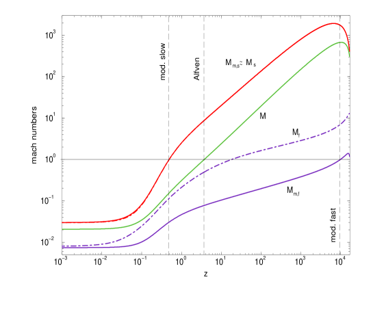
Figure 2: Plot of the various Mach numbers vs. the vertical height $z$ in units of the equatorial cylindrical radius $\varpi_{o}=\varpi(z=0)$ of a particular fieldline. A polytropic radially self-similar model is used with the parameters of model I (Tab. 2). The critical transitions at the three singularities are marked with vertical lines.

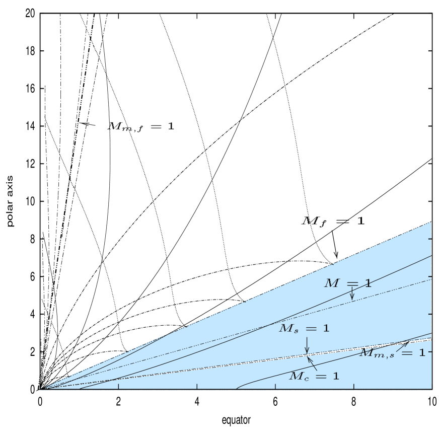
Figure 3: Poloidal fieldlines (solid), characteristics (dotted and dot-dashed) and cones of the singular surfaces (dot-dot-dashed) are shown for the radially self-similar polytropic solution of model I. In the shadowed regions the governing partial differential equations are of elliptic type and no characteristics exist. The parameters are as in Fig. 2.

In Fig. 2 we plot the various Mach numbers along each field line $\alpha$ vs. the vertical height $z$ in units of the equatorial cylindrical radius $\varpi(z=0)$ of a particular fieldline and for model I. The various critical transitions are indicated, and on the disk surface we find $G_{o}\approx 0.16$ and $M_{o}\approx 0.02$. The SMSS almost coincides with the point where the flow becomes superslow magnetosonic ($M_{\rm s,m}\approx M_{\rm s}=1$), at $z\approx 0.5$. The Alfvén critical point ($M=1$) is crossed at $z\approx 3.5$ while the wind becomes superfast magnetosonic ($M_{\rm f}=1$) at $z\approx 20$. Much farther away is the FMSS, at $z\approx 10^{4}$. Downstream of this position the various Alfvén numbers decrease, as expected from the previous topological analysis.

The turning of the solutions is evident in Fig. 3, where the poloidal streamlines together with the characteristics are plotted. They cross all critical surfaces, and for $\theta<\theta_{\rm m,f}$ the fieldlines converge towards the symmetry axis such that the conical region with $\theta<\theta_{\rm m,f}$ is causally disconnected from the rest of the domain. The two families of the characteristics in the hyperbolic domain bounded by the cusp and slow surfaces are better seen in Fig. 4 obtained for the adiabatic case, with a different set of parameters. One family of characteristics (black) is tangent to the SMSS at $M_{\rm m,s}=1$ while the other (grey) crosses it. Similarly, in the hyperbolic domain bounded by the cone where $M_{\rm f}=1$ one of the family of the characteristics (black) is tangent to the FMSS indicated by $M_{\rm m,f}=1$ while the other (grey) crosses it. We remind that the cusp surface ($M_{\rm c}=1$) does not coincide with any singularity or typical velocity in the flow.

The components of the outflow speed along a line $\alpha=const$ in units of the initial $z$-component of the flow speed at the disk, are plotted in Fig. 5. The units are choosen in order to make a direct comparison of this solution with other solutions in the literature (e.g. BP82). Close to the disk level, the escape speed is high, $V_{\rm esc,o}\approx 440$, the initial rotational speed is lower, $V_{\rm\phi,o}=110$ and of the order of the Keplerian speed, $V_{\rm Kep}\sim 3V_{\rm\phi,o}$. The azimuthal speed $V_{\phi}$ after some increase in the region of corotation, approximately up to the Alfvén critical point at $z\sim 4$, decays to zero transferring its corresponding kinetic energy to poloidal motion. Thus, the $z$- and $\varpi$-components of the poloidal motion grow from their subslow and subescape values at the disk level where $V_{z}=1$ to the high values obtained at the modified fast critical point where $V_{z}\sim 10^{3}$. The poloidal speed exceeds the local escape speed around the Alfvén transition. A comparison of model I and II makes clear that the different values of $x$ do not strongly affect the global behaviour of the solutions, even though the boundary conditions of the disk are rather different.

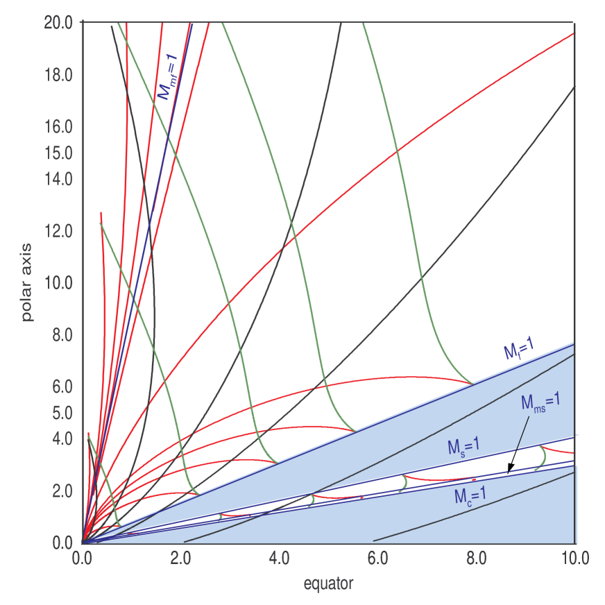
Figure 4: Poloidal fieldlines (solid) and characteristics (gray, black) for a radially self-similar polytropic (adiabatic) model with $x=0.75$, $\gamma=5/3$, $\theta_{\star}=60^{\circ}$, $\psi_{\star}=45^{\circ}$, $\kappa^{2}=15$, $\mu=10.9239$, $\lambda^{2}=2.7935$, $p_{\star}=-5.5744$, $\epsilon=9.4487$. The cones of the different transitions are shown, as well as the regions where equations are elliptical (shaded).

Figure 5: Plot vs $z$ of the components of the outflow speed for model I (solid) and model II (dashed), with the parameters given in Tab. 2.

Downstream of the Alfvén transition the azimuthal component of the magnetic field grows to very high values in comparison to the poloidal component (Fig. 6). At the modified fast critical point practically all the magnetic flux is in the azimuthal direction. For example, $B_{\phi}/B_{P}\approx 1$ at the disk, while $B_{\phi}/B_{P}\approx 60$ after the modified fast transition for both, models I and II. From Fig. 6 it may be also seen that the flow velocity is largely in the $z$-direction with very small components along $\hat{\phi}$ and $\hat{\varpi}$. In Fig. 6, the main difference between the two models is in the region upstream of the SMSS: for $x=0.75$ the angle between the poloidal fieldline and the disk surface is $\psi_{o}\approx 67^{\circ}$, while for $x=0.7525$ this angle is $\psi_{o}\approx 56^{\circ}$. Although these values are not very different, only the second case matches the outflow launching condition for a cold plasma given in BP82. This means that magnetocentrifugal driving is more efficient in model II at the base. However, we note that at the SSMS where the plasma pressure has dropped significantly both solutions can be magneto-centrifugally accelerated. The end result shown in Fig. 5 is that the terminal speed is lower when $x$ is larger, i.e., when the ejection index is higher. This result is consistent with Ferreira’s (1997) analysis.

The behaviour of the various components of the conserved total energy $E$ vs. $z$, plotted in Fig. 7, provides information on the different driving mechanisms that govern the dynamics of the outflow. Upstream of the SMSS and close to the base, most of the energy flux is electromagnetic plus some amount of enthalpy. The kinetic energy of the plasma is negligible. As the slow magnetosonic surface is approached, the kinetic energy sharply increases with a corresponding decrease of the thermal energy. Downstream of the Alfvén surface the Poynting flux rapidly decreases; the poloidal kinetic energy keeps increasing, becoming largely the main component of the energy flux at the position of the FMSS. This behaviour is basically the same for both models I and II. In order words, there is some contribution to the acceleration of thermal origin up to the modified slow critical point after which the pressure drops to a rather constant value while the magnetic pressure maintains considerably higher values up to the Alfvén transition.

Figure 6: Plot vs. $z$ of the ratios of the magnetic components $B_{\phi}/B_{p}$ and poloidal flow speeds $V_{z}/V_{\varpi}$ for models I and II (solid and dashed lines), with the parameters given in Table 2.

Figure 7: Plot vs. $z$ of the various components of the conserved total energy $E$ for model I.

We conclude this section by pointing out that the two solutions we have analyzed here correspond to efficient magnetic rotators in the terminology of Bogovalov & Tsinganos (1999), since the ratio of the corotational velocity to the poloidal Alfvén velocity at the Alfvén critical surface (the parameter $\alpha$ in their notation) has a value greater than unity ($\approx 2.13$).

5 Discussion

Before discussing the main physical implications of our results, also in connection with those obtained by other authors, we show that the present solutions are suitable to describe the physical properties of astrophysical outflows.

5.1 Astrophysical applications

The modeling of a particular astrophysical outflow requires first the calculation of all physical quantities from the non dimensional parameters characterizing the particular model. We will address here this question of calculating some observable quantities of disk-winds associated with protostellar objects from the parameters of our model.

We deduce first the ratios of some characteristic speeds at the disk level, keeping in mind that from the numerical results we have obtained $M_{o}\sim 0.01$ and $G_{o}\sim 0.1$. We will refer in the following mainly to the solutions with $x=0.75$.

First, the ratio of the poloidal Alfvén and Keplerian speeds at the disk level is:

$$\left(\frac{V_{Ap}}{V_{\rm Kep}}\right)_{o}=0.316\times\left(\frac{M_{o}}{0.01}\right)\left(\frac{G_{o}}{0.1}\right)^{-3/2}\frac{1}{\kappa\sin\psi_{o}}\approx 0.178\,.$$ (21)

The poloidal magnetic field which is essential in the launching of the outflow is anchored in the disk and its energy density is less than the rotational kinetic energy density of the disk. Thus, the field is rather weak to brake the rotation of the plasma at the disk and it is carried passively around by azimuthal rotation.

Second, the ratio of the sound and initial speeds at the disk level is:

$$\left(\frac{C_{s}}{V_{o}}\right)_{o}=70.7\times\left({\gamma\mu}\right)^{1/2}\left(\frac{G_{o}}{0.1}\right)^{2}\frac{10^{-4}}{M_{o}^{(\gamma+1)}}\approx 94\,,$$ (22)

where $V_{o}=V_{z}(z=0)$. The initial ejection speed is negligible in comparison to the thermal speed at the disk, a situation similar to a thermally driven wind.

Next, the ratio of the sound and Keplerian speeds at the disk level is:

$$\left(\frac{C_{s}}{V_{\rm Kep}}\right)_{o}=0.22\times(\gamma\mu)^{1/2}\left(\frac{G_{o}}{0.1}\right)^{1/2}\frac{1}{\kappa M_{o}^{(\gamma-1)}}\approx 0.314\,.$$ (23)

We notice that the Keplerian speed is about 3 times higher than the thermal speed at the disk. Thus, thermal effects cannot inhibit the rotation of the disk.

Finally, the ratio of the Keplerian and initial speeds at the disk level is:

$$\left(\frac{V_{\rm Kep}}{V_{o}}\right)_{o}=316\times\kappa\left(\frac{G_{o}}{0.1}\right)^{3/2}\left(\frac{10^{-2}}{M_{o}}\right)^{2}\approx 300\,,$$ (24)

i.e., the initial speed is negligible in comparison to the Keplerian speed.

In our case the flow speed at the fast critical point is about $10^{3}$ the initial speed $V_{o}$. In agreement with the observations we can reasonably assume the terminal speed of the outflow to be $\sim 400$ km s^-1, such that its velocity at the base is $V_{o}=$ 0.4 km s^-1.

In principle, radially self-similar models do not have an intrinsic scale length; however from the previous estimate of the initial speed one allows to calculate the footpoint of the reference fieldline $\alpha=1$ on the disk. In units of 10 solar radii this cylindrical distance $\varpi_{o}$ is:

$$\frac{\varpi_{o}}{10R_{\odot}}=0.19\times\left(\frac{M_{o}}{0.01}\right)^{4}\left(\frac{0.1}{G_{o}}\right)^{3}\frac{1}{\kappa^{2}}\frac{\cal M}{\cal M_{\odot}}\left(\frac{V_{o}}{{\rm km}\,{\rm s}^{-1}}\right)^{-2}.$$ (25)

Hence, for a one solar mass star we get $\varpi_{o}\approx 12.5R_{\odot}$.

It is also interesting to calculate the mass-loss rate $\dot{\cal M}_{w}$ in units of $10^{-8}{\cal M}_{\odot}\,{\rm yr}^{-1}$ :

$$\begin{array}[]{l}\displaystyle\frac{\dot{\cal M}_{w}}{10^{-8}{\cal M_{\odot}}\,{\rm yr}^{-1}}=0.0386\times\left(\displaystyle\frac{M_{o}}{0.01}\right)^{2}\left(\frac{B_{z,o}}{10G}\right)^{2}\times\\ \\ \left(\displaystyle\frac{\varpi_{o}}{10R_{\odot}}\right)^{2}\left(\displaystyle\frac{V_{o}}{\rm km\,{\rm s}^{-1}}\right)^{-1}f(\alpha_{out},\alpha_{in})\,,\end{array}$$ (29)

where

$$f(\alpha_{out},\alpha_{in})=\frac{\alpha_{out}^{x-3/4}-\alpha_{in}^{x-3/4}}{x-3/4}\qquad{\rm if}\quad x\neq 0.75\,,$$ (30)

and

$$f(\alpha_{out},\alpha_{in})=\ln\frac{\alpha_{out}}{\alpha_{in}}\qquad{\rm if}\quad x=0.75\,.$$ (31)

By assuming $\varpi_{in}=\varpi_{o}$, $\varpi_{out}\approx 10\varpi_{o}$ and $B_{z,o}=8$ G we have ${\dot{\cal M}_{w}}/(10^{-8}{\cal M_{\odot}}\,{\rm yr}^{-1})\approx 1$, with a temperature at the base of the flow of:

$$T_{o,in}=3\times 10^{5}\mu\left(\frac{G_{o}}{0.1}\right)^{4}\frac{10^{-8}}{M_{o}^{2(\gamma+1)}}\left(\frac{V_{o}}{{\rm km}\,{\rm s}^{-1}}\right)^{2}\approx 8\times 10^{4}\,{\rm K}\,,$$ (32)

$$T_{o,out}=T_{o,in}\frac{\varpi_{in}}{\varpi_{out}}\approx 8\times 10^{3}\,{\rm K}\,.$$ (33)

We remind that $T_{o}$ is not the temperature of the disk as we have assumed a transition layer between the disk surface and the base of the flow (see Sec. 2). This region could be reasonably related to a corona heated by dissipative processes in the plasma (e.g. magnetic reconnection, ohmic heating, etc.; see e.g. Königl & Pudritz 2000).

As the flow corotates roughly up to the Alfvén point (Fig. 5) the specific angular momentum carried by the wind is $\dot{J}_{w}=\dot{\cal M}_{w}\Omega\varpi_{\alpha}^{2}$ while the angular momentum that has to be extracted locally at the foot point $\varpi_{o}$ of the fieldline in order that the disk accretes at a rate $\dot{\cal M}_{a}$ is $\dot{J}_{a}=(1/2)\Omega\varpi_{o}^{2}\dot{\cal M}_{a}$ (Spruit 1996). If the angular momentum carried by the wind is a fraction $f$ of $\dot{J}_{a}$ while $1-f$ is the fraction carried away by viscous stresses, then the ratio of the mass fluxes in the wind and in the accretion flow is

$${\dot{\cal M}_{w}\over\dot{\cal M}_{a}}={f\over 2}{\varpi_{o}^{2}\over\varpi_{\alpha}^{2}}\mathrel{\hbox{\hbox to0.0pt{\hbox{\lower 4.0pt\hbox{$\sim$}}\hss}\hbox{$<$}}}0.015\,,$$

taking into account that $\varpi_{\alpha}=5.8\varpi_{o}$ for model I. It follows that the rate of the outflowing mass is at most of the order of 1$\%$ of the rate of the accreted mass; and this is achieved when the wind carries all the angular momentum of the accreted mass. When the outflow carries a smaller fraction of the angular momentum of the disk, the mass loss rate in the wind is an even smaller fraction of the mass loss rate in the wind. In other words, the mass loss rate in the wind is a negligible fraction of the accreted mass, despite that the jet may carry most of the angular momentum of the accreted mass. Similar results are obtained for the case $x=0.7525$. Therefore, from the above arguments we may conclude that from our solutions we deduce for the physical parameters values in reasonable agreement with those observed in this class of objects.

Our solution terminates at $z/\varpi_{o}\approx 2\times 10^{4}$, i.e., at $\approx 400$ Astronomical Units (AU) from the central star. At this position we could argue that there exists a shock matching the solution with the outermost region of the outflow (Gomez de Castro & Pudritz 1993). It is well known that bright knots are observed on scales of thousands AU along most protostellar jets. These configurations are shocks that are interpreted as originated either by fluid instabilities on the jet surface or by temporal variations in the velocity of the outflow (Burrows et al. 1996, Ray 1996, 1998, Micono et al. 1998, Königl & Pudritz 2000). It could be reasonable to associate the terminal shock of our solutions with the inner knots, found at distances down to $\approx 100$ AU from the star. However we cannot ignore that these knots are non steady configurations and move outwards with velocities $\sim 100\div 200$ km s^-1 (Ray 1996). We could assume that the shock is well upstream of the optical knots: polarimetric radio data on the T Tauri object are consistent with the presence of a shock at $\approx 20\div 40$ AU from the star (Ray et al. 1997). Alternatively the terminal shock could indeed be located approximately at the positions of the inner knots, but there the flow looses both self-similarity and steadiness. However as we are in the superfast magnetosonic regime, the upwind configuration is not affected. Only a much more detailed parametric study will be able to test these two possibilities.

5.2 Physical properties of the critical solutions

The solutions of this model, in particular Fig. 7, illustrate nicely the physical process of transferring electromagnetic Poynting energy flux and enthalpy to directed kinetic energy flux of the flow in order to accelerate a disk wind and then form a jet along the symmetry axis of the system. Thus, the analysis of the previous section is interesting in the sense that it reveals the driving mechanisms of the outflow. The poloidal kinetic energy is negligible at the disk level. It then increases rather sharply up to the region of the SMSS and Alfvén surfaces. This increase is at the expense of both, the enthalpy and the electromagnetic Poynting energy flux (see, Fig. 7). The poloidal velocity is directed basically in the radial direction (Figs. 5 and 6), i.e., here part of the random thermal energy together with a part of the electromagnetic energy are mostly transformed to directed wind expansion. Downstream of the Alfvén surface it is mainly the Poynting energy flux that is effectively transformed into kinetic energy directed along the rotational axis, till the FMSS is encountered. After the FMSS, the flow has already reached the maximum speed available from the total energy E, which is also approximately equal to the initial electromagnetic Poynting energy flux. Then, the acceleration asymptotically stops. Despite the fact that most of the acceleration to high speeds is apparently of magnetic origin, the role of the polytropic index and thus of the initial thermal acceleration may not be negligible, in particular in the region before the SMSS. For example, in the case of Fig. 4 where the flow is exactly adiabatic and $\gamma=5/3$, the critical solution achieves only a very small axial component of the velocity which is twice the axial velocity on the equatorial plane. In the quasi-isothermal case of models I and II where $\gamma=1.05$, the maximum velocity is 1000, higher than the equatorial one (Fig. 5). As a matter of fact, this last case is closer to the one analyzed in Li (1995) and Ferreira (1997) where the gas is isothermal up to the first critical surface and then it is taken to be cold afterwards, wherein the pressure has sufficiently dropped. However, another possibility is that the low terminal speed obtained in the adiabatic case of Fig. 4 could be due to the lower value of the rotation parameter $\lambda^{2}$ which is $\sim 2.8$ in the adiabatic case of Fig. 4, as opposed to values $\sim 137$ and 136 in models I and II and similarly for the case examined in Ferreira (1997).

When the gas has reached a high speed along the $z$-axis, its inertia causes it to lag behind the rotation of the field line and the field is wound up, as shown in Fig. 6, resulting to a highly twisted magnetic field. Consequently, the strong curvature force of this predominantly azimuthal magnetic field towards the $z$-axis, causes the poloidal field to collimate. Initially the field is flaring away from the rotation axis but the curvature force bends the poloidal field lines toward the rotation axis. The azimuthal velocity peaks around the Alfvén point which is at a height $z=3.5$ and a cylindrical distance $\varpi=5.8$ times the starting distance $\varpi_{o}$ in model I. Beyond the Alfvén point the rotation drops in accordance to angular momentum conservation and thus the centrifugal force becomes negligible. Then, the strong inwards curvature force of the twisted field, wins, over the weak outwards centrifugal force and gas pressure gradient with the result that the lines are bent and eventually collapse towards the rotation axis.

It is interesting that this feature of the collapse of the outflow towards the rotation axis which appears in cold models (BP82) and models that do not cross the FMSS (Li 1995, Ferreira 1997), is also preserved in the present hot model where also all critical points are crossed. This result seems to indicate the rather dominant role of the magnetic hoop stress in radially self-similar models, contrary to what happens in meridionally self-similar models wherein the structure becomes asymptotically cylindrical (Trussoni et al. 1997, Sauty et al. 1999, Vlahakis & Tsinganos 1999).

It is worth to clarify for a moment the term “disk-wind” that we used in this study. By that term we simply intend to indicate that we describe an outflow from a disk-like structure accreting onto a central gravitational object. Thus, the flow starts at some angle $\theta_{o}$ above or at the equatorial plane of the disk, as opposed to a “stellar” wind flow that starts radially above or at a spherical or quasi-spherical source. Needless to say that a consistent solution of the accreting part of the flow would be required for a consistent solution of the inflow-outflow structure in the case of a disk-wind. However, such a complete undertaking is beyond the scope of the present paper which only intends to emphasize the possibility to construct complete steady self-similar solutions for the wind crossing all critical points.

To make such a connection between the disk and the outflow, in the spirit of BP82, Li (1995) and Ferreira (1997), the first step would be to see how our parameters may fall into the range of parameters considered by those models. For that purpose, in Eqs. (15) - (19) we have made a correspondance between our parameters and those used by BP82. Thus, in the “standard” solution of BP82 the parameters are: $\kappa_{\rm BP}=0.03$, $\lambda_{\rm BP}=30$ and $\xi^{\prime}_{o}=1.58$ corresponding to a launching angle of the jet at the disk $\psi_{o}\approx 32^{\circ}<60^{\circ}$. In our case, we find $\kappa_{\rm BP}\approx 0.13$, $\lambda_{\rm BP}\approx 14.57$, for both, model I and model II. We also have ${\xi^{\prime}_{o}}_{\rm BP}=\cot\psi_{o}=0.425$ ($\psi_{o}=67^{\circ}$) for model I and ${\xi^{\prime}_{o}}_{\rm BP}=\cot\psi_{o}=0.675$ ($\psi_{o}=56^{\circ}$) for model II, in the BP82 notation. We note that the values of $\kappa_{\rm BP},\lambda_{\rm BP}$ are close in BP82 and the present model. However, the value of the launching angle $\psi_{o}$ is $>60^{\circ}$ in our model I because of the additional thermal driving of the outflow at the disk level, contrary to the cold model of BP82 where $\psi_{o}\approx 32^{\circ}<60^{\circ}$. In summary, our models I and II occupy in the space of $\kappa_{\rm BP}$ and $\lambda_{\rm BP}$, roughly the same domain as in BP82 (cf. Fig. 2 in BP82). The only difference is in the value of the launching angle $\psi_{o}$ which can be larger in the present hot model, as expected. These values are within the range of the allowed parameters in the ($\kappa_{\rm BP}$, $\lambda_{\rm BP}$) space also in the analysis of Li (1995, cf. Fig. 3) provided that the magnetic diffusivity is of order one. Note also that model II with $x=0.7525$ corresponds to an ejection index in the notation of Ferreira (1997) $\xi=2x-3/2=0.005$.

5.3 Summary

In this paper we have extended the classical work of Blandford and Payne (1982), mainly by showing via examples for the first time that a solution passing through all MHD critical points can indeed be constructed.

As is well known, the FMSS plays the role of the MHD signal horizon such that in an outflow crossing this MHD horizon all perturbations which the outflow may encounter are convected downstream by the superfast outflow and so the steady state solution is maintained. In other words, the outflow interior to the FMSS is causally disconnected and protected against any conditions it may encounter in the interstellar or intergalactic medium towards which the jet propagates after it is launched by magnetocentrifugal forces from the surface of an accretion disk.

Unlike other analytical models which produce asymptotically cylindrically collimated outflows (Sauty & Tsinganos 1994, Trussoni et al. 1997, VT98, Sauty et al. 1999, Vlahakis & Tsinganos 1999), this class of radially self-similar models cannot continue to infinity but it has to be stopped downstream of the FMSS and matched via a MHD shock to a subfast outflow that mixes with the interstellar medium (Gomez de Castro & Pudritz 1993). This shock can connect the present solutions to some breeze, subAlfvén or subslow magnetosonic branch perhaps also preserving the self-similarity.

Thus, the main difference here with previous results presented in the literature is that the asymptotic part of the present solutions is causally disconnected from the source and hence any perturbation downstream of the superfast transition cannot affect the whole structure of the steady outflow.

This task of matching the present solutions with a downstream shock however remains a challenge for future studies, together with a (time-consuming) more extended parametric analysis and also a correct matching of the ideal MHD outflow solutions with an inflow in a non-ideal accretion disk (Ferreira 1997).

References

Bardeen J. M., Berger B. K., 1978, ApJ, 221, 105

Blandford R. D., Payne D. G., 1982, MNRAS, 199, 883 (BP82)

Bogovalov S. V., 1994, MNRAS, 270, 721

Bogovalov S. V., 1996, MNRAS, 280, 39

Bogovalov S. V., 1997, A&A, 323, 634

Bogovalov S. V., Tsinganos K., 1999, A&A, 305, 211

Burrows C. J., Stapelfeldt K. R., Watson A. M., et al., 1996, ApJ, 473, 451

Cabrit S., Edwards S., Strom S. E., Strom K. M., 1990, ApJ, 354, 687

Cabrit S., Andre P., 1991, ApJ, 379, L25

Contopoulos J., Lovelace R. V. E., 1994, ApJ, 429, 139 (CL94)

Contopoulos J., 1995, ApJ, 450, 616

Ferreira J., 1997, A&A, 319, 340

Ferreira J., Pelletier G., 1995, A&A, 295, 807

Gomez de Castro A. I., Pudritz R. E., 1993, ApJ, 409, 748

Habbal S. R., Tsinganos K., 1983, J. Geoph. Res., 88(A3), 1965

Hartigan P., Edwards S., Ghandour L., 1995, ApJ, 452, 736

Königl A., Pudritz R. E., 2000, in V. Manning, A. Boss, S. Russel, eds, Protostars and Planets IV, University of Arizona Press (astro-ph 9903168)

Lery T., Henriksen R. N., Fiege J., 1999, A&A, 350, 254

Li Z-Y., 1995, ApJ, 444, 848

Li Z-Y., 1996, ApJ, 465, 855

Micono M., Massaglia S., Bodo G., Rossi P., Ferrari A., 1998, A&A, 333, 1001

Ostriker E., 1997, ApJ, 486, 291

Ouyed R., Pudritz R. E., 1997, ApJ, 482, 712

Padgett D., Brandner W., Stapelfeldt K., Strom S., Tereby S., Koerner D., 1999, AJ, in press (astro-ph 9902101)

Parker E. N., 1958, ApJ, 128, 664

Ray T. P., 1996, in K. Tsinganos, ed, Solar and Astrophysical MHD Flows, Kluwer Academic Publishers, 539

Ray T. P., Muxlow T. W. B., Axon D. J., Brown A., Corcoran D., Dyson J., Mundt R., 1997, Nature, 385, 415

Ray T. P., 1998, in S. Massaglia, G. Bodo, eds, Astrophysical jets: Open problems, Gordon and Breach Science Publishers, 173

Sauty C., Tsinganos K., 1994, A&A, 287, 893

Sauty C., Tsinganos K., Trussoni E., 1999, A&A, 348, 327

Spruit H. C., 1996, in R.A.M. Wijers et al., eds, Evolutionary Processes in Binary Stars, Kluwer Academic Publishers, 249

Trussoni E., Tsinganos K., Sauty C., 1997, A&A, 325, 1099

Tsinganos K., 1982, ApJ, 252, 775

Tsinganos K., Sauty C., 1992, A&A, 257, 790

Tsinganos K., Sauty C., Surlantzis G., Trussoni E., Contopoulos J., 1996, MNRAS, 283, 811

Vlahakis N., Tsinganos K., 1997, MNRAS, 292, 591

Vlahakis N., 1998, Analytical Modeling of Cosmic Winds and Jets, PhD thesis, University of Crete, Heraklion

Vlahakis N., Tsinganos K., 1998, MNRAS, 298, 777 (VT98)

Vlahakis N., Tsinganos K., 1999, MNRAS, 307, 279

Weber E.J., Davis L.J., 1967, ApJ, 148, 217

Appendix

The two first order differential equations for $G(\theta)$, $M(\theta)$ governing the present class of solutions are:

$$\frac{dG^{2}}{d\theta}=\frac{2G^{2}\cos\psi}{\sin\theta\cos\left(\psi+\theta\right)}\,,$$ (34)

$$\begin{array}[]{l}\displaystyle\frac{dM^{2}}{d\theta}=-2\displaystyle\frac{\sin\left(\psi+\theta\right)}{\cos\left(\psi+\theta\right)}\left\{-\displaystyle\frac{\kappa^{2}\sin\theta}{G}-\mu\left(x-2\right)M^{4-2\gamma}+\right.\\ \\ \left.\displaystyle\frac{M^{4}}{G^{4}}\left(1-M^{2}\right)\displaystyle\frac{\cos\psi\sin\theta}{\sin\left(\psi+\theta\right)}-\displaystyle\frac{M^{4}}{G^{4}}\left(x-2\right)\displaystyle\frac{\sin^{2}\theta}{\cos^{2}\left(\psi+\theta\right)}-\right.\\ \\ \left.\displaystyle\lambda^{2}\displaystyle\frac{M^{4}}{G^{2}}\left(x-2\right)\left(\displaystyle\frac{1-G^{2}}{1-M^{2}}\right)^{2}+\displaystyle\lambda^{2}\displaystyle\frac{M^{2}}{G^{2}}\frac{G^{4}-M^{2}}{1-M^{2}}-\right.\\ \\ \left.\displaystyle\lambda^{2}\displaystyle\frac{\cos\psi}{\sin\theta\sin\left(\psi+\theta\right)}\displaystyle\frac{\left(2M^{2}-1\right)G^{4}-M^{4}}{G^{2}\left(1-M^{2}\right)}\right\}\times\\ \\ \left\{\gamma\mu\left(1-M^{2}\right)M^{-2\gamma}-2\displaystyle\lambda^{2}\displaystyle\frac{M^{2}}{G^{2}}\left(\displaystyle\frac{1-G^{2}}{1-M^{2}}\right)^{2}+\right.\\ \\ \left.2\displaystyle\frac{M^{4}\sin^{2}\theta}{G^{4}}\left(1-\displaystyle\frac{1}{M^{2}\cos^{2}\left(\psi+\theta\right)}\right)\right\}^{-1}\,.\end{array}$$ (46)

In the above two equations $\psi(\theta)$ is given by the Bernoulli integral:

$$\begin{array}[]{l}\psi=\pi-\theta\mp\arctan{}\left\{\displaystyle\frac{G^{4}}{M^{4}\sin^{2}\theta}\left[2\epsilon-\displaystyle\frac{\gamma\mu}{\left(\gamma-1\right)M^{2\left(\gamma-1\right)}}+\right.\right.\\ \\ \left.\left.\displaystyle\frac{2\kappa^{2}\sin\theta}{G}-\displaystyle\lambda^{2}\left(\displaystyle\frac{\left(G^{2}-M^{2}\right)^{2}}{G^{2}\left(1-M^{2}\right)^{2}}+2\displaystyle\frac{1-G^{2}}{1-M^{2}}\right)\right]-1\right\}^{1/2}\,.\end{array}$$ (50)

with the upper sign corresponding to the outflow case ($V_{r}>0$).

On the Alfvén conical surface for $\theta\rightarrow\theta_{\star}$ we have

$$\left(\displaystyle\frac{1-G^{2}}{1-M^{2}}\right)_{\star}=\displaystyle\frac{2\cos\psi_{\star}}{p_{\star}\sin\theta_{\star}\cos\left(\psi_{\star}+\theta_{\star}\right)}\,,$$

where $p_{\star}$ is the slope of the square of the Alfvén number. Then from Eq. (A2) we get the following third degree polynomial for $p_{\star}$:

$$\begin{array}[]{l}\left(x-2\right)\left(\displaystyle 4\lambda^{2}+p_{\star}^{2}\sin^{2}\theta_{\star}\right)\tan^{2}\left(\psi_{\star}+\theta_{\star}\right)+\\ \\ \left(p_{\star}^{3}\sin^{2}\theta_{\star}+\displaystyle 4\lambda^{2}p_{\star}+8\lambda^{2}\frac{\left(x-2\right)}{\tan\theta_{\star}}\right)\tan\left(\psi_{\star}+\theta_{\star}\right)+\\ \\ \left(x-2\right)\left(\mu p_{\star}^{2}+p_{\star}^{2}\sin^{2}\theta_{\star}+\displaystyle 4\lambda^{2}\frac{1}{\tan^{2}\theta_{\star}}\right)+\displaystyle\kappa^{2}p_{\star}^{2}\sin\theta_{\star}\\ \\ -\displaystyle\lambda^{2}p_{\star}\left(p_{\star}-\frac{4}{\tan\theta_{\star}}\right)=0\,.\end{array}$$ (58)