Detection of Strong Clustering of Extremely Red Objects: Implications for the Density of $z>1$ Ellipticals

Abstract

We present the results of a wide–field survey for extremely red objects (EROs hereafter), the widest so far, based on $Ks$ and $R$ band imaging. The survey covers 701 arcmin² and it is 85% complete to $Ks\leq 18.8$ over the whole area and to $Ks\leq 19.2$ over 447.5 arcmin². Thanks to the wide field covered, a complete sample of about 400 EROs with $R-Ks\geq$5 was selected. The distribution of the EROs on the sky is strongly inhomogeneous, being characterized by overdensities and large voids. We detect at the $8\sigma$ level a strong clustering signal of the EROs which is about an order of magnitude larger than the clustering of $K$-selected field galaxies in the same magnitude range. A smooth trend of increasing clustering amplitude with the $R-Ks$ color is observed. These results are strong evidence that the largest fraction of EROs is composed of high–$z$ ellipticals, of which we detect for the first time the $z\lower 2.15277pt\hbox{$\;\buildrel>\over{\sim}\;$}1$ large scale structure clustering signal. We show how the surface density variations of the ERO population found in our survey can explain the highly discrepant results obtained so far on the density of $z>1$ ellipticals, and we briefly discuss the main implications of our results for the evolution of elliptical galaxies. The number counts and the colors of the $K$-selected field galaxies are also presented and briefly discussed.

1 Introduction

Near-infrared surveys prompted the discovery of a population of objects with very red optical-infrared colors (Extremely Red Objects, EROs hereafter; e.g. Elston et al. 1988, McCarthy et al. 1992, Hu & Ridgway 1994; Thompson et al. 1999; Yan et al. 2000; Scodeggio & Silva 2000). In general, objects have been classified as EROs when they had redder colors than late type galaxies (with negligible dust extinction) at any redshift. However, depending on the depth of the photometry and on the available filters, different selection criteria have been used to select EROs. In this paper, EROs are defined as objects with $R-Ks\geq$5 (see Sect. 5 for more details on this choice).

The red colors of EROs are consistent with two classes of galaxies: they could be old, passively evolving elliptical galaxies at $z\lower 2.15277pt\hbox{$\;\buildrel>\over{\sim}\;$}1$ which are so red because of the large $K$–correction. EROs may also be strongly dust–reddened star–forming galaxies or AGN. The observational results of the last few years showed that both classes of galaxies are indeed present in the ERO population: on one hand, a few objects were spectroscopically confirmed to be $z>1$ ellipticals (Dunlop et al. 1996, Spinrad et al. 1997, Liu et al. 2000, and marginally, Soifer et al. 1999), or to have surface brightness profiles consistent with being dynamically relaxed early type galaxies (e.g. Stiavelli et al. 1999, Benitez et al. 1999). On the other hand, other EROs have been detected in the sub–mm (Cimatti et al. 1998, Dey et al. 1999, Smail et al. 1999, Andreani et. al. 2000), thus providing examples of high–redshift starburst galaxies reddened by strong dust extinction and characterized by high star formation rates. The relative contribution of the two classes of objects to the whole ERO population is still unknown, but there are preliminary indications, based on near-IR and optical spectroscopy and on surface brightness analysis, that ellipticals may represent the largest fraction of this population (e.g. Cimatti et al. 1999, 2000; Liu et al. 2000; Moriondo et al. 2000). A small fraction of low-mass-stars and brown dwarfs among EROs is also expected in case of unresolved objects (e.g. Thompson et al. 2000, Cuby et al. 1999).

The importance of studying EROs is clear especially for the clues that they could provide on the formation and evolution of elliptical galaxies. For instance, existing realizations of hierarchical models of galaxy formation predict a significant decline in the comoving density of the ellipticals with $z$, as they should form through merging at $z\lower 2.15277pt\hbox{$\;\buildrel<\over{\sim}\;$}2$ (Kauffmann 1996, Baugh et al. 1996a), so that a measure of a decline of their comoving density would provide a stringent proof of these models. Conflicting results have been found so far about such issue: some works claim the detection of a deficit of $z>1$ ellipticals (e.g. Kauffmann et al. 1996, Zepf 1997, Franceschini et al. 1998, Barger et al. 1999, Menanteau et al. 1999), whereas others find that a constant comoving density of ellipticals up to $z\sim 2$ is consistent with the data (Totani & Yoshii 1997, Benitez et al. 1999, Broadhurst & Bowens 2000, Schade et al. 1999). A potentially serious problem in these studies is suspected to be the influence of the field-to-field variations in the density of EROs due to the small fields of view usually covered in the near-infrared. For instance, Barger et al. (1999) found a very low surface density of EROs in a 60 arcmin² survey to $K=20$, while on a similar area McCracken et al. (1999) observed a density three times larger at the same $K$ level.

Similar uncertainties have been found in the attempts of deriving the fraction of high redshift galaxies among IR selected samples, which is believed to be a stringent test for the formation of the massive galaxies (Broadhurst et al. 1992, Kauffmann & Charlot 1998). Fontana et al. (1999), using photometric redshifts, found that the fraction of high–$z$ galaxies in a collection of small deep fields complete to $K=21$ was low and comparable with the predictions of the cold dark matter (CDM) models, but not with passive evolution (PLE) models. The preliminary results of Eisenhardt et al. (2000), suggesting a much higher fraction of high–$z$ galaxies, are instead consistent with both CDM and PLE models.

The main aim of our survey was to encompass the difficulties induced by the cosmic variance, obtaining a sample of EROs on a large area, at moderately deep $K$ levels, in order to minimize and possibly to detect the effects of their clustering, and to compare the observed density with that expected in the case of passive evolution of ellipticals. Our survey is larger by more than a factor of four than the Thompson et al. (1999) survey, and by more than an order of magnitude than all the other previous surveys for EROs, at the same limiting magnitudes. With the large area covered we aimed also to detect a sample, or place limits to the surface density of the very rare class of extreme EROs with $R-Ks\geq 7$.

In this paper, the observational results of this survey and their main implications are presented. A more detailed interpretation of our findings will be presented in a forthcoming paper (Daddi et al., in preparation).

The paper is organized as follows: we first describe the data reduction and analysis, then we present the counts of field galaxies. In Sect. 4 the sample of EROs is described. Sect. 5 contains the analysis of the clustering of field galaxies and EROs. The main implications of our findings are discussed in Sect. 6. H${}_{\rm 0}=50$ km s^-1 Mpc^-1 throughout the paper.

2 Observations, data reduction and photometry

2.1 $Ks$-band imaging

The $Ks$ observations were made with the ESO NTT 3.5m telescope in La Silla, during the nights of 27–30 March 1999, using the SOFI camera (Moorwood et al. 1998) with a field of view of about 5$\arcmin\times$5$\arcmin$. SOFI is equipped with a Hawaii HgCdTe 1024x1024 array, with a scale of 0.29$\arcsec$/pixel. The $Ks$ filter has $\lambda_{\rm c}=2.16\leavevmode\nobreak\ \mu m$ and $\Delta\lambda\sim 0.3\leavevmode\nobreak\ \mu m$ and it is slightly bluer than the standard $K$ filter in order to reduce the thermal background.

The center of the observed field is at $\alpha$ = 14^h49^m29^s and $\delta$ = 09$\degr 00\arcmin 00\arcsec$ (J2000). The observed field is one of the fields described in Yee et al. (2000) to which we refer for details about its selection. The main criteria were not to have any apparent nearby clusters and to be at high galactic latitude.

The images were taken with a pattern of fixed offsets of 144$\arcsec$ (about half of the SOFI field of view) over a grid of 9$\times$13 pointings. The total area covered by the observations was about 24$\times$34 arcmin, with a local integration time of 12 minutes in the central deepest region of the field. In the shallower region, the effective integration time is reduced to not less than 6 minutes. The total amount of time required to cover the whole field was about 5.5 hours.

The data reduction was carried out using the IRAF software. The images were flat-fielded with twilight flats. The sky background was estimated and subtracted for each frame using a clipped average of 6–8 adjacent frames (excluding the central frame itself). The photometric calibration was achieved each night with the observation of 5-7 standard stars taken from Persson et al. (1998). The zero-points have a scatter of $\sim$ 0.015 magnitudes in each night and a night-to-night variation within 0.02 magnitudes. Each frame was scaled to the same photometric level correcting for the different zero-points and airmasses. Accurate spatial offsets were measured for each frame using the area in common with the adjacent frames. The images were then combined, masking the known bad pixels, in order to obtain the final mosaic. The cosmic rays were detected and replaced by the local median using the task cosmicrays of the IRAF package ccdred. The effective seeing of the final coadded mosaic ranges from 0.9$\arcsec$ to 1.1$\arcsec$.

2.2 $R$-band imaging

The $R$-band data were taken in May 19–21 1998 with the 4.2m William Herschel Telescope on La Palma. The observations were done using the prime focus camera, equipped with a thinned 2048x4096 pixels EEV10 chip, with a scale of 0.237$\arcsec$/pixel. This gives a field of view of about 8.1$\arcmin\times 16.2\arcmin$. A standard Johnson $R$–filter was used. The whole field has been covered by a mosaic of 6 pointings. Each pointing consisted of at least 3 exposures of 1200s taken with small offsets. The total integration times per pointing was therefore 3600s, with the exceptions of two pointings with 4800s and 6000s.

The photometric calibration was achieved with standard stars taken from Landolt (1992) with a scatter in the zeropoints, from the different stars used, below 0.01 magnitudes. The images were de-biased and then flatfielded, using a master flatfield constructed from the science exposures, scaled to the same zeropoint and then combined. The seeing of the final $R$-band mosaic was between 0.7$\arcsec$ and 0.8$\arcsec$.

2.3 Sample selection and $Ks$ photometry

The software SExtractor (Bertin & Arnouts 1996) was run on the $Ks$ mosaic with a background weighted threshold in order to take into account the depth variations across the area, as defined by SExtractor. Among the detected objects, all those with S/N$>5$ in a 2^′′ circular aperture (twice the average seeing FWHM) were selected and added to the catalog. A few spurious detections (e.g. close to image defects) have been excluded after a visual inspection of the image. The final catalog includes 4585 objects. In the central deepest region, the 5$\sigma$ limiting aperture magnitude is $Ks$(2^′′)=19.6, whereas in the remaining area such limit is $Ks$(2^′′)$\;\buildrel>\over{\sim}\;$19.2 because of the reduced integration time.

Isophotal magnitudes were measured with a limiting threshold of about 0.7$\sigma_{\rm sky}$ corresponding in the central area to a surface brightness limit of about $\mu_{\rm lim}\sim 21$ mag arcsec^-2. The aperture correction from 2^′′ to total magnitudes was estimated throughout the area by measuring the difference between the isophotal and the 2$\arcsec$ aperture magnitudes for the stars with $Ks<$16. A differential correction, in the range of 0.16–0.30 magnitudes, was measured for different regions of the mosaic with a typical scatter less than 0.03 magnitudes. For the bright objects the isophotal magnitudes were on average consistent with the Kron automatic aperture magnitudes. However, we adopted the isophotal magnitudes because the Kron magnitudes are rather unstable at faint flux levels, where the low signal often does not allow to define the correct automatic aperture.

The total $Ks$ magnitudes were then defined as the brightest between the isophotal and the corrected aperture magnitude. This allowed to safely assign a total magnitude for both the faint and the bright objects. The typical $Ks$ magnitude where the corrected aperture magnitude begins to be adopted as the total one is $Ks$$\sim$18 in the central deepest region.

The completeness of our catalog has been estimated by adding artificial objects to the $Ks$ mosaic in empty positions, using the IRAF package artdata. Point-like sources as well as objects with De Vaucouleurs and exponential profiles (convolved with the seeing PSF) were simulated, and SExtractor was run with the same detection parameters as for the real data. The 85% completeness magnitude for the deepest area is $Ks=19.2$ for point-like sources. The completeness decreases to $\sim$ 70% for the worst case that we have tested, i.e. for exponential galaxies with 0.7$\arcsec$ half–light radius. In the shallower area the corresponding limiting magnitude is $Ks\leq 18.8$. Most of the $Ks\lower 2.15277pt\hbox{$\;\buildrel>\over{\sim}\;$}18.5$ galaxies are anyway expected to be only barely resolved with the $Ks$ 1$\arcsec$ seeing (Saracco et al. 1997), and this certainly occurs for the distant $z\lower 2.15277pt\hbox{$\;\buildrel>\over{\sim}\;$}1$ ellipticals, and thus their completeness limits can be assumed to be similar to those for stars.

2.4 $R$-band photometry and colors

In order to recover the $R$-band counterparts of the $Ks$-selected objects, a coordinate mapping between the $Ks$ and the $R$ images was derived. SExtractor was then run in ASSOC mode with a search box of 2$\times$ FWHM_R. The regions around bright stars or defects in the $R$ and $Ks$ band images were excluded from this analysis. The final effective area is 701 arcmin² at $Ks\leq 18.8$ and 447.5 arcmin² at $18.8<Ks\leq 19.2$.

Whenever an object had S/N$<$3 in the $R$-band image 3$\sigma$ limits were assigned. The 3$\sigma$ limiting magnitude in a 2$\arcsec$ diameter aperture is $R>26.2$ for most of the area, reaching $R>26.5$ in the deepest pointing. When S/N$>$3, 2$\arcsec$ diameter corrected aperture magnitudes were assigned to each object. The aperture correction was derived in the same way as for the $Ks$-band, with slightly smaller corrections because of the better $R$-band seeing. The magnitudes were dereddened for Galactic extinction. At the Galactic coordinates of the center of our field ($l\sim 5\aas@@fstack{\circ}5$, $b\sim 57\degr$), the extinction coefficients from Burstein & Heiles (1982) and from Schlegel et al. (1998) are $A_{\rm B}=0.04$ and $A_{\rm B}=0.13$ respectively. Since the two values are derived in different ways, neither of the two can be discarded. The average was therefore adopted, obtaining a correction of 0.052 magnitudes in $R$ and negligible in $Ks$. This introduces an uncertainty of $\sim$ 0.03 magnitudes in the dereddened $R$ magnitudes.

Figure 1: The observed number counts for both stars and galaxies in our survey. The error bars indicate the poissonian uncertainties.

Finally, the $R-Ks$ colors are defined for all the objects as the difference between the $R$ and $Ks$ corrected aperture magnitudes. Thanks to the depth of the $R$-band data, colors as red as $R-Ks=7$ could be measured down to the $Ks$ magnitude limits of our survey. Because of the long integrations used in the $R$-band the objects with $R\lower 2.15277pt\hbox{$\;\buildrel<\over{\sim}\;$}20$ were saturated. This effect is obviously more important for stars than for galaxies; moreover, since we are interested in the extremely red galaxy population, the effects due to saturation have no impact on our results.

2.5 Star–Galaxy classification

The star–galaxy (S/G) separation was done by means of the SExtractor CLASS_STAR parameter in both the $R$ and $Ks$ band. This classification was found to be reliable for objects with $Ks\lower 2.15277pt\hbox{$\;\buildrel<\over{\sim}\;$}$17.5 and $R\lower 2.15277pt\hbox{$\;\buildrel<\over{\sim}\;$}$24. Because of the seeing variations through the area in both bands, a variable CLASS_STAR threshold was adopted in different subareas. Given the better seeing of the $R$-band, the classification was based mostly on that band, switching to the $Ks$ CLASS_STAR for objects close to the saturation level in $R$. Objects which are fainter than $Ks$ = 17.5 and $R$ = 24 have not been classified and have been considered to be galaxies. This means that a S/G separation can be provided only for objects with colors $R-Ks\lower 2.15277pt\hbox{$\;\buildrel<\over{\sim}\;$}$5 at $Ks$=19, $R-Ks\lower 2.15277pt\hbox{$\;\buildrel<\over{\sim}\;$}$6 at $Ks$=18, and so on (see Fig. 5 and the upper panel of Fig. 3). From the small number of objects classified as stars which are close to the diagonal straight line which indicates our S/G classification limit in the color - magnitude plane, we can safely conclude that our inability to properly classify very red, faint objects has almost no effect on the total star number counts and, therefore, on the galaxy number counts. In addition, it is possible that near the faint limit of our survey a very small fraction of very compact, blue galaxies, such as for instance AGN or compact narrow emission line galaxies (e.g. Koo & Kron 1988), could have been incorrectly classified as stars.

3 $Ks$-band number counts

Galaxy number counts in the $Ks$ band can provide more advantages in studying galaxy evolution and cosmological geometry than optical counts because they are much less sensitive to the evolution of stellar population and to the dust extinction. Our survey, which covers the magnitude range $14<Ks<19.2$, represents the widest among the previous deep surveys at levels fainter than $Ks>18$.

Table 1: Differential Number Counts

$Ks$ range	Area[2]	Galaxies	Stars
11.7 – 12.2	701	-	4
12.2 – 12.7	”	-	7
12.7 – 13.2	”	-	9
13.2 – 13.7	”	-	17
13.7 – 14.2	”	4	21
14.2 – 14.7	”	6	38
14.7 – 15.2	”	16	37
15.2 – 15.7	”	30	62
15.7 – 16.2	”	74	73
16.2 – 16.7	”	100	88
16.7 – 17.2	”	178	128
17.2 – 17.7	”	372	127
17.7 – 18.2	”	633	144
18.2 – 18.7	”	892	185
18.7 – 18.8	”	200	32
18.8 – 19.2[1]	447.5	628	84

^[1] The last bin includes only the objects in the deepest region.
^[2] arcmin²

Table 1 summarizes the number of galaxies and stars detected in each $Ks$ bin and Fig. 1 shows the corresponding differential counts in 0.5 magnitude bins. No correction for incompleteness was applied. Galaxies start to dominate over stars at $Ks\sim 16.5$ and their surface density is about a factor of 8 higher than the stellar surface density at $Ks\sim 19.$

Figure 2: Counts of galaxies from our survey compared to a collection of published data. The solid curve shows the average counts as estimated by Hall & Green (1998).

The slopes of the galaxy number counts were derived over the magnitude range covered by our survey. At bright magnitudes a slope of $\gamma=0.53\pm 0.02$ is found in the range $14<Ks<17.5$. We confirm that the $K$-band galaxy counts show a flattening at $Ks\sim 17.5$, where the best fit slope changes from $\gamma=0.53$ to $\gamma=0.32\pm 0.02$ (see Fig. 2). The leveling off of the counts below a slope of 0.4 indicates that the differential contribution to the extragalactic background light (EBL) in the $K$ band peaks at $Ks\sim 17-18$ and then starts to decrease at fainter fluxes. The contribution to the EBL over the magnitude range $14\leq Ks\leq 19.2$ sampled by our survey is about $4.20$ nW/m²/sr, which constitutes about $53\%$ of the estimated EBL from discrete sources in the $K$-band (cf. Pozzetti et al. 1998, Madau & Pozzetti 2000).

Fig. 2 shows the differential galaxy number counts in our survey compared with a compilation of $K$-band published surveys. No attempt was made to correct for different filters. As shown in the figure, our counts are in very good agreement with the average counts of previous surveys (Hall & Green 1998).

Table 2: Galaxy Median Colors

$Ks$ range	Galaxies	Median $R-Ks$
16.5 – 17.0	143	3.54
17.0 – 17.5	277	3.80
17.5 – 18.0	522	3.92
18.0 – 18.5	759	4.08
18.5 – 18.8	613	4.11
18.8 – 19.2	628	4.04

Figure 3: Color magnitude diagram for the stars (upper panel) and galaxies (lower panel) samples. The diagonal straight line in the upper panel indicates our S/G classification limit in the color - magnitude plane (see text). The bluer objects plotted with filled squares have at least one pixel close to saturation in the $R$-band. Some of the bluest saturated galaxies at $Ks>17$ may actually be stars. The reddest galaxies with $R-Ks\lower 1.72221pt\hbox{$\;\buildrel>\over{\sim}\;$}7$ have color lower limits as they are not detected in the $R$-band (see Fig. 5).

Figure 4: Distributions of the $R-Ks$ colors for the galaxies of our sample.

4 The sample of EROs

Table 3: The Sample of EROs

	area	$R-Ks$$\geq$5			$R-Ks$$\geq$5.3			$R-Ks$$\geq$6			$R-Ks$$\geq$7
$Ks$ limits	arcmin2	N	Frac.	Dens.	N	Frac.	Dens.	N	Frac.	Dens.	N	Frac.	Dens.
$Ks\leq$17.0	701	2	0.006	0.003	–	–	–	–	–	–	–	–	–
$Ks\leq$17.5	701	15	0.025	0.02	5	0.008	0.007	–	–	–	–	–	–
$Ks\leq$18.0	701	58	0.051	0.08	19	0.017	0.027	–	–	–	–	–	–
$Ks\leq$18.5	701	158	0.084	0.23	75	0.040	0.11	7	0.004	0.01	–	–	–
$Ks\leq$18.8	701	279	0.111	0.40	150	0.060	0.21	30	0.012	0.04	2	0.0008	0.003
$Ks\leq$19.0	447.5	220	0.116	0.49	133	0.070	0.30	33	0.017	0.07	4	0.0021	0.009
$Ks\leq$19.2	447.5	281	0.126	0.63	173	0.079	0.39	44	0.020	0.10	5	0.0023	0.011
$Ks\leq$19.2	701+447.5	279+119	0.127	0.67	150+87	0.076	0.40	30+27	0.018	0.10	2+4	0.0019	0.012

We present in detail the cumulative number (N) of EROs selected at each $Ks$ limiting magnitude, the fraction of EROs with respect to the whole field galaxies (Frac.) and the corresponding surface density (Dens., in objects/arcmin²). The last line was calculated using the whole survey area to $Ks=18.8$ and the deeper area to $Ks=19.2$. The data presented here are used throughout the paper.

Figure 5: Enlarged portion of Fig. 3 (bottom) around the reddest colors. Filled boxes are objects within the completeness limits of our survey ($Ks\leq 19.2$ in the deeper area and $Ks\leq$18.8 outside) while filled triangles are objects fainter than those limits. The horizontal long-dashed lines correspond to the limits reported in Table 3 for the selection of the samples of EROs. In the region above the short-dashed line the star–galaxies separation is not feasible. The objects along the diagonal dotted lines are not detected in $R$ and have a 3$\sigma$ limit in that band.

In Fig. 3 the $R-Ks$ vs. $Ks$ color - magnitude diagram is plotted for both stars and galaxies in our sample. The diagonal straight line in the upper panel indicates our S/G classification limit in this plane. Because objects above this line are not classified, no star can appear in the upper right corner. However, this figure shows that there are very few stars with a color redder than $R-Ks>5$, even in the region of this color - magnitude diagram where our morphological classification is still reliable. This suggests that very few stars should be present in the sample of objects for which no morphological classification was possible.

Fig. 4 shows the distribution of colors for galaxies fainter than $Ks=16.5$, from which the median color at different $Ks$ magnitude levels have been calculated (see Table 2). In spite of the presence of objects with color upper and lower limits, the use of the median colors (instead of the mean colors) allows unbiased estimates in the $Ks$ range we are considering. The faintest bin with 18.8$<Ks\leq$19.2 includes only the objects detected in the deeper region. The median $R-Ks$ color of the galaxies increases by 0.5 magnitudes from $Ks=16.5$ to $Ks\sim 18$ and then it remains almost constant up to the limits of our survey ($Ks$=19.2). This trend is similar to what is found by Saracco et al. (1999) for the median $J-Ks$ galaxies color, which also reaches a maximum at $Ks\sim$ 18–19 and then it becomes bluer, while the median $B-K$ color gets significantly bluer at brighter ($K\sim 17$) magnitudes (Gardner et al. 1993).

Our wide-field survey allows us to select a statistically significant and complete sample of EROs which can provide stringent constraints on the density of high-$z$ ellipticals (see Sect. 1). For this reason, EROs are defined as objects with $R-Ks\geq 5$ because this corresponds to select passively evolving ellipticals at $z\lower 2.15277pt\hbox{$\;\buildrel>\over{\sim}\;$}0.9$ (see Fig. 13). Table 3 shows the results of the selection for different magnitude and color thresholds. Among the others, the threshold $R-Ks\geq 5.3$ is used because it corresponds to the selection of $z\lower 2.15277pt\hbox{$\;\buildrel>\over{\sim}\;$}1$ elliptical galaxies (see Fig. 13). We detected 279 EROs with $Ks\leq 18.8$ from the whole area and 119 EROs with $18.8<Ks\leq 19.2$ in the deeper area, yielding a total sample of 398 objects (see Fig. 5 and Table 3). This is by far the largest sample of EROs obtained to date. A small but complete sample of EROs with $R-Ks\geq 7$ has also been selected, and we estimate for the first time their surface density to be $\sim 0.01$ arcmin^-2 at $Ks\sim 19$.

A comparison of the surface densities of the EROs in our sample with those in the Thompson et al. (1999) survey can be directly done after taking into account the different filters used in the two surveys. For the $K^{\prime}$ filter used by Thompson et al. (1999), $Ks$ $\sim$ $K^{\prime}$ - 0.2 (adopting $H-K=1$), and therefore their limit at $K^{\prime}\leq 19$ corresponds to $Ks\leq 18.8$ which is the shallower limit of our survey, while their $R-K^{\prime}$ color is bluer than our $R-Ks$ by about 0.1 magnitudes for the redder objects (Thompson, private communication). At the level of $Ks\leq 18.8$ we find a density of $0.042\pm 0.008$ arcmin^-2 for EROs with $R-Ks\geq 6$, to be compared with the value of 0.039$\pm$0.016 that they find (these errors are poissonian). Thus, the two surface densities are in excellent agreement with each other. We also verified that the average $R-Ks$ color of all our objects with $17.8<Ks<18.8$ ($R-Ks=3.70\pm 0.03$, determined with a Kaplan-Meier estimator), is in good agreement with the average $R-K^{\prime}=3.73\pm 0.04$ in $18<K^{\prime}<19$ by Thompson et al. (2000).

5 The angular correlation functions

Statistical measurements of the clustering of faint galaxies are important for studying the evolution of galaxies and the formation of structures in the Universe. In fact, the amplitude of clustering in 2D space is a useful probe of the underlying 3D structure (e.g. Connolly et al. connolly (1998), Efstathiou et al. 1991, Magliocchetti & Maddox 1999). The clustering of galaxies on the sky has been studied extensively especially in the optical, but also in the near-infrared (e.g. Roche et al. 1998 and 1999, Postman et al. 1998, Baugh et al. 1996b). Our survey, as noted before, is the widest at the limits of $Ks\sim 19$. It is therefore interesting to estimate the clustering of our sample of galaxies.

5.1 Calculation technique

The angular two-point correlation function $w(\theta)$ is defined as the excess probability (over a poissonian distribution) of finding galaxies separated by the apparent distance $\theta$:

$$dP=N^{2}[1+w(\theta)]d\Omega_{\rm 1}d\Omega_{\rm 2}$$ (1)

where N is the mean density per steradian (Groth & Peebles, 1977).

Several methods for estimating $w(\theta)$ from a set of object positions have been proposed and used, but the most bias–free and suitable for faint galaxies samples resulted to be the Landy & Szalay technique (Landy & Szalay 1993, see also Kerscher et al. 2000). This technique (adopted for the calculations in this paper) consists in deriving the counts of objects binned in logarithmic distance intervals, for the data-data sample $[DD]$, the data-random sample $[DR]$ and the random–random sample $[RR]$. These counts have to be normalized, i.e. divided for the total number of couples in each of the 3 samples. From them we can estimate $w_{\rm b}(\theta)$ as:

$$w_{\rm b}(\theta)=\frac{[DD]-2[DR]+[RR]}{[RR]}$$ (2)

which is biased to lower values with respect to the real correlation function $w(\theta)$:

$$w(\theta)=w_{\rm b}(\theta)+\sigma^{2}$$ (3)

where $\sigma^{2}$ is the ”integral constraint” (Groth & Peebles, 1977):

$$\sigma^{2}=\frac{1}{\Omega^{2}}\int\int w(\theta)d\Omega_{\rm 1}d\Omega_{\rm 2}$$ (4)

Assuming that the angular correlation function $w(\theta)$ can be described by a power law of the form $w(\theta)=A\theta^{-\delta}$, then, following Roche et al. (1999), we can extimate the ratio between $\sigma^{2}$ and the amplitude $A$ using the random–random sample:

$$C=\frac{\sigma^{2}}{A}=\frac{\sum N_{\rm rr}(\theta)\theta^{-\delta}}{\sum N_{\rm rr}(\theta)}$$ (5)

The amplitude of the real two-point correlation function $w(\theta)$ can then be estimated by fitting to the measured $w_{\rm b}(\theta)$ the function:

$$w_{\rm b}(\theta)=A(\theta^{-\delta}-C)$$ (6)

The errors can be estimated, following Baugh et al. (1996b), as:

$$\delta w_{\rm b}(\theta)=2\ \sqrt[]{(1+w_{\rm b}(\theta))/DD)}$$ (7)

where $DD$ is the non normalized histogram of $[DD]$. Eq. (7) is equivalent to assuming 2$\sigma$ poissonian errors for the correlations, and it gives estimates that are comparable to the errors obtained with the bootstrap technique (Ling, Frenk & Barrow 1986). This is necessary because it is known that, as the counts in the different bins are not completely independent, assuming the 1$\sigma$ poissonian errors would result in an underestimate of the true variance of the global parameters of the angular correlation (see Mo et al. 1992).

In case of the presence of a randomly distributed spurious component among the analyzed sample of objects (an example of this case would be a residual stellar component among the galaxy sample), the resulting amplitudes are apparently reduced by a factor $(1-f)^{2}$, where $f$ is the fraction of the randomly distributed component (see e.g. Roche et al. 1999), and the corresponding correction should be applied.

Figure 6: The observed, bias–corrected two-point correlation functions of our $K$–selected sample. The lines plotted are the best–fitted power laws (see Table 4). The error in each bin is two times the poissonian error (see Sect. 5.1).

Table 4: Clustering amplitudes for the $K$–selected sample

$Ks$ limit	area	Galaxies	A[10-3]	$\delta$	C
18.0	701	1131	1.3$\pm$0.5	0.8	4.55
18.5	701	1890	1.6$\pm$0.3	0.8	4.55
18.8	701	2503	1.5$\pm$0.2	0.8	4.55
19.2	447.5	2222	1.6$\pm$0.2	0.8	5.16

The random samples used in our analysis were obtained using the pseudo–random number generator routine of the C Library function drand48. Random samples with up to 200 000 objects were used. Typically the number of objects in the random samples were a factor of 100–200 larger than the number of observed objects. The random sample was generated with the same geometrical constraints as the data sample, avoiding for instance to place objects in the regions excluded around the brightest stars.

5.2 The clustering of the $K$-selected field galaxies

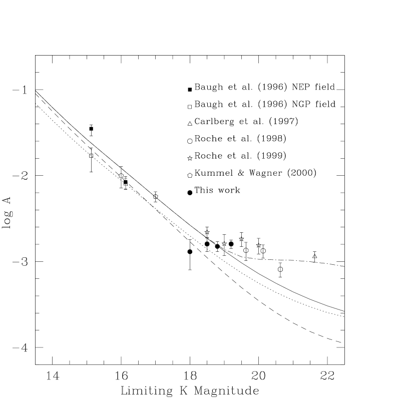
Figure 7: The clustering amplitudes measured in our survey, compared with published data from the literature. The models shown here are from Roche et al. (1998) and Fig. 7 of Roche et al. (1999).

In our analysis a fixed slope of $\delta=$ 0.8 was assumed, as this is consistent with the typical slopes measured in both faint and bright surveys (e.g. Baugh et al. 1996b, Roche et al. 1996, Maddox et al. 1990), and because it gives us the possibility to directly compare our results with the published ones that are typically obtained adopting such a slope. The factor $C$ was estimated (with Eq. (5)) for both the whole and the deeper areas, turning out to be 4.55 and 5.16 respectively (the angles are expressed in degrees, if not differently stated). In Fig. 6 the observed, bias corrected, two-point correlation functions $w(\theta)$ are shown; the bins have a constant logarithmic width ($\Delta\log\theta=0.2$), with the bin centers ranging from 3.6$\arcsec$ to 15$\arcmin$.

We clearly detect a positive correlation signal for our sample with an angular dependence broadly consistent with the adopted slope $\delta=$ 0.8, even if the measurements show some deviations, in particular for the brightest samples. A few cluster candidates are present in our survey. These possible clusters include galaxies with $R-Ks\leq 4.5$, and are therefore expected to be at $z\lower 2.15277pt\hbox{$\;\buildrel<\over{\sim}\;$}0.6$. A detailed analysis of the cluster candidates will be given in a forthcoming paper. For the purpose of the present work, we tested that the measured clustering amplitudes are stable in case of removal of the galaxies of the most evident cluster from the sample. However, the presence of such clusters, most of which happen to be in the shallower area, could partly explain the observed deviations from the fitted $w(\theta)=A\ \theta^{-0.8}$ power laws for the three brightest samples.

Figure 8: The sky positions of the objects with $Ks\leq$18.8 and $R-Ks$$\geq$5 in our survey. The region enclosed within the dashed line is the deeper region. The colors of the objects inside the circle are shown in Fig. 11.

The derived clustering amplitudes are presented in Table 4. The amplitude errors are obtained from the fit assuming Eq. (7). No correction for the stellar contamination was applied. In Fig. 7 the clustering amplitudes of our samples are compared with other published measurements. The data are shown together with a number of PLE models with different clustering evolutions, which are described in detail in Roche et al. (1998, 1999). Our measurements are in good agreement with both the models and the previous estimates of Roche et al. (1999), except for the point with limiting magnitude $Ks=18.0$, which is however the most uncertain of our data points.

As a check it was verified that the correlations of the stellar sample are consistent with zero, within the measured errors, at all the scales. This is a confirmation that the stars are homogeneously distributed on the field (as they should be) and the seeing variations across the area did not cause a detectable bias in our classification.

5.3 The clustering of the extremely red objects

Table 5: Clustering amplitudes for the Extremely Red Objects

	area	$R-Ks\geq 5$ sample		$R-Ks\geq 5.3$ sample
$Ks$ limit	arcmin2	Galaxies	A[10-3]	Galaxies	A[10-3]	$\delta$	C
18.0	701	58	24$\pm$10	–	–	0.8	4.55
18.25	701	106	25$\pm$5	–	–	0.8	4.55
18.5	701	158	22$\pm$3	–	–	0.8	4.55
18.8	701	279	14$\pm$2	150	14$\pm$3.4	0.8	4.55
19.2	447.5	281	13$\pm$1.5	173	12$\pm$2.3	0.8	5.16

The large sample of EROs derived from our survey allowed us for the first time to estimate their clustering properties. Even a simple visual inspection of the sky distribution of the objects with $R-Ks\geq 5$ (see Fig. 8) shows that the EROs have a very inhomogeneous distribution.

Figure 9: The observed, bias–corrected two-point correlations for the sample of EROs (with $R-Ks$$\geq$5) in our survey. As in Fig. 6, the error in each bin is twice the poissonian one. Because of the small number of objects included, some bins for the two brightest samples, at small angular separation, were not populated. The corresponding upper limits would be in agreement with the fitted amplitudes.

The results of the quantitative analysis of the clustering are shown in Fig. 9, where the observed, bias–corrected angular correlations $w(\theta)$ of the objects with $R-Ks$$\geq$5 are displayed. A strong clustering is indeed present at all the scales that could be measured, and its amplitudes (Table 5) are about an order of magnitude higher than the ones of the field population at the same $Ks$ limits. The correlations are very well fitted by a $\delta=0.8$ power law. No attempt was made to correct the amplitudes for the stellar contamination (see Sect. 5.1), and we stress that such corrections would increase them. Adopting the errors derived from the fits, our detections are significant at more than 7$\sigma$ level for the samples with $R-Ks\geq 5$ and $Ks$ limits equal to or fainter than $Ks=18.5$.

The amplitudes shown in Fig. 5 suggest a possible trend of decreasing strength of the clustering for fainter EROs: the $Ks\leq$19.2 EROs are less clustered than the ones with $Ks\leq$18.5 and the difference is significant at $2.7\sigma$, based on the derived errors. The significance of this effect would, however, decrease if the contamination by randomly distributed stars increases towards the limit of our survey. Although difficult to be quantified, this is likely to happen because, differently from the brightest EROs, only a small fraction of the EROs fainter than $Ks$ = 18.5 could be morphologically classified (see Fig. 5).

Defining redder thresholds drastically reduces the number of EROs and it is not possible to estimate with sufficient accuracy how the amplitudes change for objects with even redder $R-Ks$ colors. We could only verify that the sample of EROs with $R-Ks\geq 5.3$ has clustering amplitudes consistent with those of the $R-Ks\geq 5$ samples (see Table 5). To measure the clustering of the $R-Ks\geq$6 EROs, an area at least 10 times larger than ours (i.e. $\sim$2 square degrees) at $K=19$ would be needed, assuming that their clustering amplitudes are similar to those of the EROs with $R-Ks\geq 5$.

Finally, it was studied if and how the clustering amplitude changes as a function of $R-Ks$ for the $Ks\leq$18.8 sample (see Fig. 10). A clear increase of $A$ with $R-Ks$ is present for colors $R-Ks$$\geq$3.5, while the $R-Ks\geq$3 sample has an amplitude that is consistent with that of the whole sample of field galaxies. The variation of $A$ can be described with a power law in the range of $3\leq R-Ks\leq 5.7$. Previous efforts to disentangle the clustering properties of the red and blue populations in faint $K$–selected samples probably failed because the ERO population was not sufficiently sampled. For instance, Kummel & Wagner (2000) did not find significant differences in the clustering of objects with color bluer or redder than $R-Ks$=3.49 for their $K<$17 sample. This is not surprising since at K$<$17 the ERO population is almost absent (see Table 3 and Fig. 3).

Figure 10: The measured correlation amplitude for the samples with $R-Ks$ redder than a fixed threshold, in function of the threshold itself. This was obtained with the $Ks\leq$18.8 sample. The horizontal lines show the $\pm 1\sigma$ range for the clustering of the whole population of field galaxies at this level. The fitted power law (dashed line) is $logA=0.43(R-Ks)-4.04$.

To check for the stability of these results, possible systematics that could produce a bias in our work were analyzed. First af all, as the clustering of our $Ks$–selected galaxies is in good agreement with the literature data (Fig. 7), we can exclude the presence of measurable biases coming from the selection of the sample.

Regarding the color measuraments, since EROs are the tail of objects in the $R-Ks$ color distribution, systematic variations of the photometric zeropoints across the area could have the effect of creating artificial ERO overdensities and voids. To exclude this possibility we verified that the blue tail of the $R-Ks$ distribution is homogeneously spread across our survey, with a very low clustering amplitude. In case of zeropoints variations these should produce the same effect in both the tails of the color distribution. Moreover, to test the reality of the large void of EROs clearly seen in the bottom region of our survey (see Fig. 8), the $R-Ks$ color distribution of the galaxies inside and outside this large void were compared by means of a Kolmogorov-Smirnov test, selecting only the galaxies with $R-Ks\leq$4 in both regions. The probability that the two distributions are extracted from the same population is 43%. Thus, the two regions are fully consistent with each other with respect to the color distribution of the blue population. This, together with the fact that no underdensity is present in this region when only the bluer galaxies are considered, shows that the void of EROs should be considered a real feature.

All these tests strongly suggest that the inhomogeneous ERO distribution is a real effect.

6 Main implications

6.1 On the nature of EROs

The strong clustering signal that we find to increase with the $R-Ks$ threshold and to reach very high values for the EROs is potentially capable of giving insight about the nature of these objects.

The main possible source of objects that may contribute to the ERO population, as discussed in the introduction, are old passively evolving $z\lower 2.15277pt\hbox{$\;\buildrel>\over{\sim}\;$}1$ ellipticals, dust-reddened starburst galaxies and, in case of unresolved objects, low-mass stars or brown dwarfs. Our field being at high galactic latitude ($b\sim 57\degr$), stars are expected to have no clustering, and to be homogeneously distributed, and certainly not to give the strong clustering signal detected. As for the starburst galaxies, it must be noted that in such galaxies the red colors are mainly driven by the amount of dust extinction and not by the redshift, as in the case of ellipticals (see Fig. 13), and therefore a wide redshift distribution is expected which should dilute their intrinsic clustering. Moreover, it is known that the IRAS–selected galaxies (which are typically star–forming galaxies) have very low intrinsic clustering (e.g. Fisher et al. 1994). We can therefore reasonably conclude that the observed signal is due to the clustering of high redshift ellipticals. This is also suggested by studies of the local universe which have shown that early-type galaxies are much more clustered than late-type galaxies (e.g. Guzzo et al. 1997, Willmer et al. 1998). In this regard the results plotted in Fig. 10 could be qualitatively explained by noting that in selecting redder samples the fraction of early type galaxies increases (the color of local ellipticals is just around $R-Ks\lower 2.15277pt\hbox{$\;\buildrel<\over{\sim}\;$}3$) and by assuming that these galaxies are intrinsically more clustered, while such plot would be difficult to understand if mainly driven by the strongly reddened starburst galaxies. These considerations strongly suggest that EROs are mainly composed by $z\lower 2.15277pt\hbox{$\;\buildrel>\over{\sim}\;$}1$ ellipticals, confirming the previous indications that had been found on this issue.

As the elliptical galaxies are the dominant population of galaxy clusters, we investigated the possibility that the detected clustering of EROs could be the result of a few massive clusters at $z\geq 1$ present in our field. For example, in the region inside the circle in Fig. 8, a large ERO overdensity is found, that one could suspect to be due to a high-$z$ cluster of galaxies. However, Fig. 11 shows that there is no clear color-magnitude sequence among the $R-Ks>5$ objects inside that region, suggesting that they do not all belong to a single cluster. In case of a cluster, even at high–$z$, a well defined color-magnitude sequence is in fact generally observed (e.g. Stanford et al. 1998). In the last years a few examples of massive $z\lower 2.15277pt\hbox{$\;\buildrel>\over{\sim}\;$}$1 clusters of galaxies have been discovered (e.g. Stanford et al. 1997, Rosati et al. 1999), with X ray luminosity of $\sim 10^{44}$ erg s^-1. A crude estimate of the number of structures of this sort that could be observed in our survey can be derived by calculating the number of high–$z$ clusters with L${}_{\rm X}>10^{44}$ erg s^-1 expected in the volume we are sampling. From the X ray luminosity function of such structures at $z\sim 1$ (Rosati et al. 2000) we estimate that the expected number of massive clusters in our field in the redshift interval $0.9<z<2$ is only $\sim 0.1$ (for $\Omega_{\rm 0}=1$).

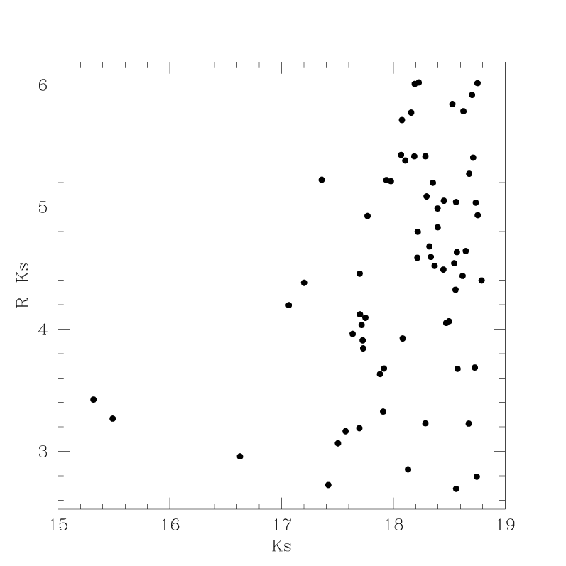
Figure 11: Color magnitude diagram of all the objects with $Ks\leq$18.8 in the region inside the circle of Fig. 8.

Moreover, the detection of the ERO positive correlation, following a $\delta=0.8$ power law on all the scales from 10$\arcsec$ to 15$\arcmin$ (corresponding to $\sim$8 Mpc at $z\sim 1$) suggests that the clustering signal does not come from a few possible clusters detected in our field, but rather from the whole large scale structure traced by the elliptical galaxies.

6.2 Fluctuations of the ERO number density

Our results on the clustering of EROs have important consequences on the problem of estimating the density of high-$z$ ellipticals (see Sect. 1).

Figure 12: The histogram shows the frequency distributions of the number of EROs ($R-Ks$$\geq$5 and $Ks\leq 18.8$) that have been recovered by sampling our survey with a SOFI field (25 arcmin²). The mean expected value is 10. The dotted curve represents the probability distribution expected in the poissonian case.

The existence of an ERO angular correlation with $\delta=0.8$ and with a high amplitude implies significant surface density variations around the mean value even for relatively large areas. In the presence of a correlation with amplitude A, the rms fluctuations of the counts around the mean value $\overline{n}$ is (see for example Roche et al. 1999):

$$\sigma_{true}^{2}=\overline{n}\ (1+\overline{n}AC)$$ (8)

The factor $C$ is the same as in Eq. (5) and, by applying Eq. (5) for several areas, it was found that it can be approximated as:

$$C=58\ {\rm Area}^{-0.4}$$ (9)

if the area is expressed in arcmin² and $\delta=0.8$. The validity of such an approximation has been tested for square regions and for areas not larger than the ones of our survey. With Eq. (8) and (9) the expected variations of the ERO number counts can be calculated, once their clustering amplitude is known.

To verify the consistency of this picture, we derived the distribution of the number of EROs (with $R-Ks$$\geq$5 and $Ks\leq$18.8, i.e. those in Fig. 8) that can be recovered in our area by sampling it with a field of view of 5$\arcmin\times$5$\arcmin$, which is the typical field of view of a near-infrared imager such as SOFI. In Fig. 12 the observed frequencies of the number of EROs recovered in this counts-in-cell analysis is plotted. As the mean expected number of EROs is about 10, the poissonian fluctuations would be $\sigma_{\rm poisson}\sim$3.2, while fluctuations with $\sigma=$5.4 are actually observed. Applying Eq. (8), the measured clustering amplitude $A=0.013$ implies $\sigma=5.55$, in excellent agreement with the measured $\sigma$ value.

We also note that the distribution of the numbers of EROs in Fig. 12 is not only asymmetric, but also very broad, ranging from $N$=0 to $N$=30. In 29% of the cases the number of EROs recovered is $N\leq$5, corresponding to a surface density half of the real one, while only in 19% of the cases the observed number is $N\geq$15. This shows that, on average, it is more probable to underestimate the real surface density of these objects. This is a clear property of the sky distribution that we observe, as the voids extend on a large fraction of the surveyed area. These results show how strong the effects of the field-to-field variations are in the estimate of the sky surface density of EROs. In this respect, it should be noted here that all previous estimates of the number density of high–$z$ ellipticals were based on surveys made with small fields of view, typically ranging from 1 arcmin² in the case of the NICMOS HDF-S (Benitez et al. 1999) to 60 arcmin² in the case of Barger et al. (2000).

6.3 Implications for the evolution of elliptical galaxies

The selection of galaxies with colors $R-Ks>5$ can be used to search for elliptical galaxies at $z>0.9$ (see Fig. 13), and to study their evolution by comparing their observed surface densities with those expected from PLE or hierarchical models of massive galaxy evolution. In this respect, very discrepant results have been obtained so far, making the formation of spheroids one of the most controversial problems of galaxy evolution (see the Introduction).

Our results on the ERO clustering clearly show that for such a comparison to be reliable, both a wide field survey (resulting in a large number of EROs) and a consistent estimate of their surface density fluctuations are necessary before reaching solid conclusions on the evolution of elliptical galaxies.

In this section, with the main aim to show the effect of the increased uncertanties due to the clustering, a preliminary comparison is presented between the sky density of EROs observed in our survey (Table 3) and the predictions of an extreme PLE model similar to that used by Zepf (1997). In this model, ellipticals formed at $z_{\rm f}$=5 and their star formation rate ($SFR$) is characterized by an exponentially decaying burst with $SFR\propto exp(t/\tau)$, with $\tau=0.1$ Gyr. Adopting the Markze et al. (1994) local luminosity function of ellipticals, and the Bruzual & Charlot (1997) models with solar metallicity and Salpeter IMF, the expected surface densities of passively evolving ellipticals with $R-Ks\geq 6$ was calculated for different limiting $Ks$ magnitudes.

Figure 13: The color–redshift relation for the extreme PLE model described in the test, computed for a flat and an open universe ($\Lambda=0$). The horizontal dashed lines are the thresholds adopted in this paper. The vertical line shows that $z>1$ ellipticals correspond to the $R-Ks>5.3$ EROs. At $z=1$ a $Ks=19$ elliptical galaxy has $L\sim 0.3L_{\rm*}$ and $L\sim 0.5L_{\rm*}$ in our flat and open models, respectively.

Figure 14: The observed integral number densities of EROs with $R-Ks$$\geq$6 (Table 3) are compared with the extreme PLE model described in the text. The three error bars shown here are, from left to right, the 1$\sigma$ poisson uncertainty and the 2$\sigma$ and 1$\sigma$ true uncertanties. The true uncertanties take into account the observed clustering of EROs.

Fig. 14 shows the comparison between the expected and the observed densities of EROs with $R-Ks\geq 6$ (such a color threshold should select passively evolving galaxies at $z\lower 2.15277pt\hbox{$\;\buildrel>\over{\sim}\;$}1.3$). For each data point we show three different error bars, which are actually the region of confidence in the poissonian case (at 1$\sigma$) and in the true (i.e. clustering corrected) case (at 1$\sigma$ and 2$\sigma$). Such confidence regions have been estimated, following the prescriptions of Eq. (8), by finding the range of values for the true average counts $\overline{n}$ for which the observed $N$ would represent a deviation of the required number of $\sigma$ from the real density. In other words such ranges are defined from the two solutions of the equation:

$$\alpha^{2}=\frac{(\overline{n}-N)^{2}}{\overline{n}(1+\overline{n}AC)}$$ (10)

where $\alpha$ is the number of $\sigma$ considered. The amplitudes of the angular correlation function used for the $R-Ks\geq 6$ EROs are those derived for the $R-Ks\geq 5$ EROs, which is likely to be a conservative assumption as the amplitudes of redder samples should be higher, as suggested by Fig. 10.

Fig. 14 shows that the observed EROs densities are indeed lower than the predictions of this particular PLE model. However, even for the most deviant point, this PLE model can be rejected at only the 2.5$\sigma$ and 2.3$\sigma$ level for $\Omega_{\rm 0}=1$ and $\Omega_{\rm 0}=0.1$ respectively, if we use the “correct” error bars. Note that the different points plotted in that figure are not statistically independent because they are partially obtained with the same objects (they are cumulative values).

It should be recalled here that the observed ERO densities plotted in Fig. 14 are an overestimate of the true density of the ellipticals because of the contamination by dusty starbursts (see Cimatti et al. 1998, 1999; Dey et al. 1999; Smail et al. 1999) and by field low-mass stars. The fraction of dusty starbursts in complete ERO samples is not known yet, as discussed in the introduction, but our results show that they should not be the dominant population. For instance, assuming that the fraction of dusty starbursts and low-mass stars is 20% and 10% of the ERO population respectively, this would decrease the observed densities plotted in Fig. 14 accordingly, but it would also increase by a factor of 2 the clustering amplitudes of the high-$z$ ellipticals (see Sect. 5.1), and hence the error bars related to those points. As a consequence, the statistical significance of the difference between data and model in this case would be only at the 2$\sigma$ level.

It is relevant to mention that the predictions of the PLE models depend very strongly on many parameters that have to be adopted a priori such as $H_{\rm 0}$, $\Omega_{\rm 0}$, the local LF of ellipticals (uncertain by up to a factor of 2), the redshift of formation $z_{\rm f}$, the history of star formation, the metallicity, the IMF, the spectral synthesis models. For instance, even just a decrease of $z_{\rm f}$, or a small residual star formation at z $\sim$ 1.5 (Menanteau et al. 98, Jimenez et al. 99), would decrease the predicted numbers of EROs making them more consistent with our data. We therefore conclude that it seems premature to reject even extreme PLE models at a high level of statistical significance on the basis of these data.

A preliminary comparison of our results can be made with some aspects of the hierarchical models of galaxy formation. First of all, our findings could qualitatively fit into the predictions of such models, where high-$z$ ellipticals should be very clustered (Kauffmann et al. 1999) because they are expected to be linked to the most massive dark matter haloes which are strongly clustered at high–$z$. The indication (marginally significant at $\sim 2.7\sigma$ level) of a decrease of the clustering amplitude of the EROs with the $Ks$ magnitude (see Sect. 5.3), if mainly due to the mass of the galaxies, could also fit well in this framework because smaller objects should be connected to smaller dark matter haloes which are expected to be less correlated. On the other hand, our results seem to conflict with the predictions made by Kauffmann & Charlot (1998) on the fraction of $K$-selected galaxies with $K\leq 19$. In fact, the fraction of galaxies observed to have color $R-Ks\geq 5.3$ (which corresponds to the selection of $z\lower 2.15277pt\hbox{$\;\buildrel>\over{\sim}\;$}1$ ellipticals) is about 7% of the total in our survey (see Table 3), to be compared with the 2–3% of $z>1$ galaxies with K$\leq$19 expected in the Kauffmann & Charlot (1998) hierarchical model. This result on the fraction of $z\lower 2.15277pt\hbox{$\;\buildrel>\over{\sim}\;$}1$ galaxies in our $K$-selected sample broadly agree with the finding of Eisenhardt et al. (2000).

7 Summary

The main results of this work are:

• We have presented a survey which covers 701 arcmin² and is 85% complete to $Ks\leq 18.8$ over the whole area and to $Ks\leq 19.2$ over 447.5 arcmin²; the R-band limit is $R\geq 26.2$ at the 3$\sigma$ level.

• The observed galaxy counts are derived over the largest area so far published in the range of $18\leq Ks\leq 19.2$. Such counts are in excellent agreement with other published data.

• The median $R-Ks$ color of field galaxies increases by 0.5 mags from $Ks=16.5$ to $Ks=18$, and it remains constant to $Ks=19.2$.

• A sample of 398 EROs has been selected. This sample is the largest published to date and is characterized by an area larger by about four times than previous surveys. The ERO counts and surface densities have been derived for several color thresholds and $Ks$ limiting magnitudes. In particular, we find $0.67\pm 0.03$ (poissonian) EROs arcmin^-2 with $R-Ks\geq 5$ and $0.10\pm 0.01$ EROs arcmin^-2 with $R-Ks\geq 6$ at $Ks\leq 19.2$.

• The surface density of EROs with $R-Ks\geq 7$ has been estimated for the first time to be of the order of $\sim 0.01$ arcmin^-2 at $Ks\sim 19$.

• The angular correlation function of field galaxies, fitted with a fixed slope $\delta=0.8$, has an amplitude $A(1\degr)\sim 0.0015$ at $18.5\leq Ks\leq 19.2$, in agreement with previous measurements.

• For the first time, we detected the clustering of EROs, with an amplitude $A(1\degr)\sim 0.015$ for the objects with $R-Ks\geq 5$, in the range $18.5\leq Ks\leq 19.2$) which is about a factor of ten higher than that of field galaxies. The ERO two point correlations are very well fitted by a $\delta=0.8$ power law.

• The clustering amplitude of the galaxies increases with the $R-Ks$ color threshold following the relation  $logA\propto 0.43(R-Ks)$, for $3\leq R-Ks\leq 5.7$ at $Ks\leq 18.8$.

• The strong clustering of EROs is shown to be a direct evidence that a large fraction of these objects are indeed high–$z$ ellipticals. Our result is therefore the first detection of the large scale structure traced by the elliptical galaxies at $z\sim 1$.

• The ERO clustering explains the conflicting results obtained so far on the density of high-$z$ ellipticals in terms of strong field-to-field variations affecting the surveys based on small fields of view (e.g. $5\times 5$ arcmin).

• Taking into account the clustering of EROs, even the predictions of extreme PLE models for the comoving density of high–$z$ ellipticals cannot be rejected at much more than 2$\sigma$ significance level.

- (1) Andreani P., Cimatti A., Loinard L., Röttgering H., 2000, A&A 354, L1
- (2) Barger A.J., Cowie L.L., Trentham N., et al., 1999, AJ 117, 102
- (3) Baugh C.M., Cole S., Frenk C.S., 1996a, MNRAS 283, 1361
- (4) Baugh C.M., Gardner J.P., Frenk C.S., Sharples R.M., 1996b, MNRAS 283, L15
- (5) Benitez N., Broadhurst T.J., Bouwens R.J., et al., 1999, ApJ 515, L65
- (6) Bertin E., Arnouts S., 1996, A&A 117, 393
- (7) Broadhurst T.J., Bowens R.J., 2000, ApJ 530, 53
- (8) Broadhurst T.J., Ellis R.S., Glazebrook K., 1992, Nature 355, 55
- (9) Bruzual G., Charlot S., 1993, ApJ 405, 538
- (10) Burnstein D., Heiles C., 1982, AJ 87, 1167
- (11) Carlberg R.G., Cowie L.L., Songaila A., Hu E.M., 1997, ApJ 484, 538
- (12) Cimatti A., Andreani P., Röttgering H., Tilanus R., 1998, Nature 392, 895
- (13) Cimatti A., Daddi E., di Serego Alighieri S., et al., 1999, A&A 352, L45
- (14) Cimatti A., Daddi E., di Serego Alighieri S., et al., 2000, in SPIE’s Int. Symposium, Vol. 4005, ed. J. Bergeron, in press
- (15) Connolly A.J., Szalay A.S., Brunner R.J., 1998, ApJ 499, L125
- (16) Cuby J.G., Saracco P., Moorwood A.F.M., et al., 1999, A&A 349, L41
- (17) Dey A., Graham J.R., Ivison R.J., et al., 1999, ApJ 519, 610
- (18) Djorgovski S., Soifer B.T., Pahre M.A., et al., 1995, ApJ 438, L13
- (19) Dunlop J., Peacock J., Spinrad H. et al., 1996, Nature 381, 581
- (20) Elston R., Rieke G.H., Rieke M., 1988, ApJ 331, L77
- (21) Efstathiou G., Bernstein G., Katz N., et al., 1991, ApJ 380, L47
- (22) Eisenhardt P., Elston R., Stanford S.A., et al., proceedings of the Xth Rencontres de Blois (1998) on ”The Birth of Galaxies”, ed. B. Guiderdoni et al. (astro-ph/0002468)
- (23) Fisher K.B., Davis M., Strauss M.A., et al., 1994, MNRAS 266, 50
- (24) Fontana A., Menci N., D’Odorico S., et al., 1999, MNRAS 310, L27
- (25) Franceschini A., Silva L., Fasano G., et al., 1998, ApJ 506, 600
- (26) Gardner J.P., Cowie L.L., Wainscoat R.J., 1993, ApJ 415, L9
- (27) Gardner J.P., Sharples R.M., Carrasco B.E., Frenk C.S., 1996, MNRAS 282, L1
- (28) Glazebrook K., Peacock J.A., Collins C.A., Miller L., 1994, MNRAS 266, 65
- (29) Groth E.J., Peebles P.J.E., 1977, ApJ 217, 38
- (30) Guzzo L., Strauss M.A., Fisher K.B., et al., 1997, ApJ 489, 37
- (31) Hall P.B., Green R.F., 1998, ApJ 507, 558
- (32) Hu E.M., Ridgway S.E., 1994, AJ 107, 1303
- (33) Huang J.S., Cowie L.L., Gardner J.P., et al., 1997, ApJ 476, 12
- (34) Jimenez R., Friaca A.C.S, Dunlop J.S., et al., 1999, MNRAS 305,L16
- (35) Kauffmann G., 1996, MNRAS 281, 487
- (36) Kauffmann G., Charlot S., 1998, MNRAS 297, L23
- (37) Kauffmann G., Charlot S., White S.D.M., 1996, MNRAS 283, 117
- (38) Kauffmann G., Colberg J.M., Diaferio A., White S.D.M., 1999, MNRAS 307, 529
- (39) Kerscher M., Szapudi I., Szalay A., 2000, ApJL, in press (astro-ph/9912088)
- (40) Koo D., Kron R.G., 1988, ApJ 325, 92
- (41) Kümmel M.W., Wagner S.J., A&A 353, 937
- (42) Landolt A., 1992, AJ 104,340
- (43) Landy S.D., Szalay A.S., 1993, ApJ 412, 64
- (44) Ling E.N., Barrow J.D., Frenk C.S., 1986, MNRAS 223, L21
- (45) Liu M.C., Dey A., Graham J.R., et al. 2000, AJ, in press (astro-ph/0002443)
- (46) Maddox S.J., Efstathiou G., Sutherland W.J., Loveday J., 1990, MNRAS 242, 43
- (47) Madau P., Pozzetti L., Dickinson M., 1998, ApJ 498, 106
- (48) Madau P., Pozzetti L., 2000, MNRAS 312, L9
- (49) Magliocchetti M., Maddox S.J., 1999, MNRAS 306, 988
- (50) Marzke R.O., Geller M.J., Huchra J.P., et al, 1994, AJ 108, 437
- (51) McCarthy P.J., Persson S.E., West S.C., 1992, ApJ 386, 52
- (52) McCracken H.J., Metcalfe N., Shanks T., et al., 2000, MNRAS 311, 707
- (53) McLeod B.A., Bernstein G.M., Rieke M.J., et al., 1995, ApJS 96, 117
- (54) Menanteau F., Ellis R.S., Abraham R.G., et al, 1999, MNRAS 309, 208
- (55) Minezaki T., Kobayashi Y., Yoshii Y., Peterson B.A., 1998, ApJ 494, 111
- (56) Mo H.J., Jing Y.P., Boerner G., 1992, ApJ 392, 452
- (57) Mobasher B., Ellis R.S., Shraples R.M., 1986, MNRAS 223, 11
- (58) Moorwood A., Cuby J.G., Lidman C., 1998, The ESO Messenger 91,9
- (59) Moustakas L.A., Davis M., Graham J.R., et al., 1997, ApJ 475, 445
- (60) Moriondo G., Cimatti A., Daddi E., 2000, submitted to A&A
- (61) Persson S.E., Murphy D.C., Krzeminski W., et al., 1998, AJ 116, 2475
- (62) Postman M., Lauer T.R., Szapudi I., Oegerle W., 1998, ApJ 506, 33
- (63) Pozzetti L., Madau P., Zamorani G., et al., 1998, MNRAS 298, 1133
- (64) Roche N., Eales S., 1996, MNRAS 307, 703
- (65) Roche N., Eales S., Hippelein H., 1998, MNRAS 295, 946
- (66) Roche N., Eales S., Hippelein H., Willott C.J., 1999, MNRAS 306, 538
- (67) Rosati P., Stanford S.A., Eisenhardt P.R., et al., 1999, AJ 118, 76
- (68) Rosati P., Borgani S., Della Ceca R., et al., 2000, to appear in “Large Scale Structure in the X-ray Universe”, Santorini, September 1999
- (69) Saracco P., Iovino A., Garilli B., et al., 1997, AJ 114, 887
- (70) Saracco P., D’Odorico S., Moorwood A., et al., 1999, A&A 349, 751
- (71) Scodeggio M., Silva D., 2000, A&A, in press
- (72) Schade D., Lilly S.J., Crampton D., et al., 1999, ApJ 525, 31
- (73) Schlegel D.J., Finkbeiner D.P., Davis M., 1998, ApJ 500, 525
- (74) Smail I., Ivison R.J., Kneib J.P., et al., 1999, MNRAS 308, 1061
- (75) Soifer B.T., Matthews K., Djorgovski S., et al., 1994, ApJ 420, L1
- (76) Soifer B.T., Matthews K., Neugebauer G., et al., 1999, AJ 118, 2065
- (77) Spinrad H., Dey A., Stern D., et al., 1997, ApJ 484, 581
- (78) Stanford S.A., Elston R., Eisenhardt R., et al., 1997, AJ 114, 2232
- (79) Stanford S.A., Eisenhardt P.R., Dickinson M., 1998, ApJ 492, 461
- (80) Stiavelli M., Treu T., Carollo C.M., et al., 1999, A&A 343, L25
- (81) Szokoly G.P., Subbarao M.U., Connolly A.J., Mobasher B., 1998, ApJ 492, 452
- (82) Thompson D., Beckwith S.V.W., Fockenbrock R., et al., 1999, ApJ 523, 100
- (83) Totani T., Yoshii J., 1997, ApJ 501, L177
- (84) Tresse L., 1999, in ”Formation and Evolution of Galaxies”, eds. O. Le Fevre and S. Charlot, Les Houches School Series, Springer-Verlag.
- (85) Yan L., McCarthy P.J., Weymann R.J., et al., 2000, AJ, in press
- (86) Yee H.K.C., Morris S.L., Lin H., et al., 2000, ApJS in press (astro-ph/0004026)
- (87) Willmer C.N.A., da Costa L.N., Pellegrini P.S., 1998, AJ 115, 869
- (88) Zepf S.E., 1997, Nature, 390, 377