Far infrared extragalactic background radiation: I. Source counts with ISOPHOT

Abstract

As a part of the ISOPHOT CIRB (Cosmic Infrared Background Radiation) project we have searched for point-like sources in eight fields mapped at two or three wavelengths between 90$\mu$m and 180$\mu$m. Most of the 55 sources detected are suspected to be extragalactic and cannot be associated with previously known objects. It is probable, also from the far-infrared (FIR) spectral energy distributions, that dust-enshrouded, distant galaxies form a significant fraction of the sources.

We present a tentative list of new extragalactic FIR-sources and discuss the uncertainties involved in the process of extracting point sources from the ISOPHOT maps. Based on the analyzed data we estimate the number density of extragalactic sources at wavelengths 90$\mu$m, 150$\mu$m and 180$\mu$m and at flux density levels down to 100 mJy to be 1$\cdot$10⁵ sr^-1, 2$\cdot$10⁵ sr^-1, and 3$\cdot$10⁵ sr^-1, respectively.

Strong galaxy evolution models are in best agreement with our results, although the number of detections exceeds most model predictions. No-evolution models can be rejected at a high confidence level.

Comparison with COBE results indicates that the detected sources correspond to $\ga$20% of the extragalactic background light at 90$\mu$m. At longer wavelengths the corresponding fraction is $\sim$10%.

1 Introduction

The cosmic infrared background (CIRB) consists in the far-infrared of the integrated light of all galaxies along the line of sight plus any contributions by intergalactic gas and dust, photon-photon interactions ($\gamma$-ray vs. CMB) and by hypothetical decaying relic particles. A large fraction of the energy released in the universe since the recombination epoch is expected to be contained in the CIRB. An important aspect is the balance between the UV-optical and the infrared backgrounds: what is lost by dust obscuration will re-appear through dust emission in the CIRB. Some central, but still largely open, astrophysical problems to be addressed through CIRB measurements include the formation and early evolution of galaxies, and the star formation history of the universe.

The primary goal of the ISOPHOT CIRB project is the determination of the flux level of the FIR CIRB. The other goals are the measurement of its spatial fluctuations and the detection of the bright end of FIR point source population contributing to the CIRB. The full analysis of the data from the DIRBE (Hauser et al. hauser (1998); Schlegel et al.schlegel98 (1998)) and FIRAS (Fixsen et al. fixsen98 (1998)) experiments indicated a CIRB at a surprisingly high level of $\sim$1 MJy sr^-1 between 100 and 240 $\mu$m. Preliminary results had been obtained already by Puget et al. (puget (1996)). Lagache et al. (lagache99a (1999)) detected a component of Galactic dust emission associated with warm ionized medium and the removal of this component lead to a CIRB level of 0.7 MJy sr^-1 at 140$\mu$m.

Because of the great importance of the FIR CIRB for cosmology these results definitely require confirmation by independent measurements. ISOPHOT observation technique is different from COBE: (1) with relatively small f.o.v. ISOPHOT is capable of looking at the darkest spots between the cirrus clouds; (2) ISOPHOT has good sensitivity in the important FIR window at 120 – 200 $\mu$m; (3) with the good spatial and spectral sampling ISOPHOT gives the possibility of recognizing and eliminating the emission of galactic cirrus.

In the ISOPHOT CIRB project we have mapped four low-cirrus regions at high galactic latitude at the wavelengths of 90, 150, and 180 $\mu$m (see Fig. 1). Through this multi-wavelength mapping we will try to separate the cirrus component and confirm the detection of sources at neighboring wavelengths. In addition, we have performed absolute photometry in several filters between 3.6 – 200 $\mu$m at the darkest spots of the fields. This photometry will be used (1) to secure the zero point for the maps at 90, 150, and 180 $\mu$m, and (2) to determine the contribution by the zodiacal emission using measurements of its SED at mid-IR wavelengths where it dominates the sky brightness.

This paper presents the first step in the analysis of the ISOPHOT CIRB observations. Here we will concentrate on the data reduction and the study of the point sources (galaxies) found in the FIR maps. The source counts determined in the FIR are important for the study of the star formation history of the universe and for the testing of the current models of galaxy evolution.

With recent observations at infrared and sub-mm wavelengths it has become obvious that star formation efficiencies derived from optical and UV observations only (e.g. Madau et al. madau (1996); Steidel et al. steidel (1996), steidel99 (1999); Cowie et al. cowie96 (1996), cowie97 (1997), cowie98 (1998); Hu et al. hu (1998)) underestimate the true star formation activity at high redshifts because the correction for dust extinction is unknown (e.g. Heckman et al. heckman (1998)).

IRAS has shown that in the local universe about one third of the luminosity is emitted at infrared wavelengths. In starburst galaxies the fraction can be much higher as most of the starlight is absorbed by dust and re-radiated in the infrared. In extreme sources like the hyperluminous galaxy $IRAS$ 10214+4724 the energy spectrum peaks around 100$\mu$m in the rest frame and more than 90% of the energy is emitted in the infrared and sub-mm regions. The emission maximum moves further towards sub-mm with increasing redshift, causing optical studies to seriously underestimate the true star formation activity. If the dust content is high enough the objects can remain completely undetected at optical wavelengths.

With ISO and new sub-mm instruments like the SCUBA bolometer array (Holland et al. holland99 (1999)) it has become possible to study the star formation history of the universe at infrared to sub-mm wavelengths (for reviews see e.g. Hughes et al. hughes3 (1998), hughes1 (1999)). Due to the negative $K$-correction the observed flux densities will not depend strongly on the redshift and it is possible to detect more distant galaxies (e.g. van der Werf werf (1999); Guiderdoni et al. guiderdoni97 (1997)).

Recent studies (e.g. Dunlop et al. dunlop (1994); Omont et al. omont (1996); Hughes et al. hughes97 (1997), hughes3 (1998); Stiavelli et al. stiavelli99 (1999); Abraham et al. abraham99 (1999); Lilly et al. lilly99 (1999); Blain et al. 1999a ) have shown that star formation activity remains high at $z>$1.

In observations with the SCUBA instrument at 450$\mu$m and 850$\mu$m (e.g. Hughes et al. hughes3 (1998); Barger et al. barger1 (1998); Smail et al. smail97 (1997); Blain et al. 1999a ; Eales et al. eales99 (1999); Lilly et al. lilly99 (1999)) galaxies have been detected up to redshifts $z$$\sim$5. Compared with galaxies seen in optical surveys the objects have higher dust content and the star formation rates are an order of magnitude higher. The surface density of the detected sources exceeds predictions of no-evolution models by at least one order of magnitude (Smail et al. smail97 (1997); Eales et al. eales99 (1999); Barger et al. barger99 (1999)). The number of sources detected by Eales et al. (eales99 (1999)) at 850$\mu$m above $\sim$3 mJy accounts for $\sim$20% of the CIRB detected by FIRAS (Fixsen et al. fixsen98 (1998)). Similar results were obtained by Barger et al. (barger99 (1999)). At the level of 0.5 mJy the sources contain most of the sub-mm CIRB ( Smail et al. smail97 (1997), smail98 (1999); Blain et al. 1999b ).

Kawara et al. (kawara (1998)) observerved the Lockman Hole at 95$\mu$m and 175$\mu$m using ISOPHOT. The number of sources found was at least three times higher than predicted by no-evolution models. The conclusions of the FIRBACK (Puget et al. puget99 (1999)) and ELAIS (Oliver et al. ringberg (2000)) projects are similar and at 175$\mu$m sources with $S_{\nu}$$>$120 mJy account for $\sim$10% of the CIRB detected by FIRAS.

In this article we study the number density of extragalactic sources and their contribution to the FIR background radiation using observations made with ISOPHOT. The data consist of maps made at wavelengths 90$\mu$m, 150$\mu$m and 180$\mu$m, and for some smaller areas at 120$\mu$m. The total area is close to 1.5 square degrees. Most of the regions have been observed at three wavelengths (90$\mu$m, 150$\mu$m, 180$\mu$m) some at two wavelengths (120$\mu$m and 180$\mu$m). Both the galactic foreground cirrus emission and the emission from typical extragalactic objects will reach their maxima within or near the observed wavelength range. In particular, we will be able to determine the cirrus spectrum for each region separately.

We have developed a point source extraction routine based on the fitting of the detector footprint to spatial data. The method is different from those used in most previous studies where the source detection algorithms have concentrated on the variations (off-on-off) of the detector signal as function of time. Our analysis will therefore be independent of and complementary to the previous results.

2 Observations and data processing

The observations were performed with the ISOPHOT photometer (Lemke at el. lemke (1996)) aboard ISO (Kessler et al. kessler (1996)). The maps were made in the PHT22 staring raster map mode using filters C_90, C_120, C_135, and C_180 with reference wavelengths at 90$\mu$m, 120$\mu$m, 150$\mu$m and 180$\mu$m, respectively. In this paper we study eight fields that cover a total of 1.5 square degrees (see Fig. 1). Two fields were observed at two wavelengths while the rest have observations at three wavelengths, the details are shown in Table 1. The C100 detector used for the 90$\mu$m observations consists of 3$\times$3 pixels each with the size of 43.5$\arcsec\times$43.5$\arcsec$ on the sky. The C200 detector used in the rest of the observations has a raster of 2$\times$2 detector pixels, 89.4$\arcsec\times$89.4$\arcsec$ each.

We have selected regions with low surface brightness. Some maps have redundancy i.e. the observed pixel rasters partly overlap each other. In four maps observed with filter C_90 the raster step is larger than the size of the detector, leading to incomplete sampling.

The data were first processed with PIA (PHT Interactive Analysis) program versions 7.1 and 7.2. Special care was taken to remove glitches caused by cosmic rays since these might be erroneously classified as point sources during later analysis. The flux density calibration was made using the FCS (Fine Calibration Source) measurements (FCS1) performed before and after each map. Generally the accuracy of the absolute calibration is expected to be better than 30% (Klaas et al. klaas98 (1998)). The calibration was normally applied to observations using linear interpolation between the two FCS measurements.

The data reduction from the ERD (Edited Raw Data; detector read outs in Volts) to SCP (Signal per Chopper Plateau; signal at each sky position in units V s^-1) was performed also using the so-called pairwise method (Stickel, private comm.). Instead of making linear fits to the ramps consisting of the detector read-outs one examines the distribution of the differences between consecutive read-outs. The mode of the distribution is estimated with myriad technique (Kalluri & Arce kalluri98 (1998)) and is used as the final signal for each sky position. This processing was done in batch mode. Compared with the previous PIA analysis there were some calibration differences which were possibly due to the different drift handling of the FCS measurements. For this reason the final surface brightness values in the new AAP (Astrophysical Applications Data) files were rescaled using the results of the previous interactive analysis. The subsequent analysis was carried out with both data sets but no significant differences were found in the results. The pairwise method is, however, believed to be more robust against glitches and in the following the results are based on the data reduced with this method.

Table 1: The eight fields studied here. The columns are: (1) the name of the field used in this paper, (2)-(3) coordinates of the centre of each field, (4)-(5) galactic coordinates of the field, (6) area of the map, (7) the number of raster positions observed over the map, (8) the step between adjacent raster positions in the staring mode mapping and (9)-(12) the integration time for each filter. The distance of adjacent scans was in all cases identical to the raster step used along the scan line

Field	Map Centre				Area	Rasters	Step	$t_{\rm int}$ (s)
	RA(2000.0)	DEC(2000.0)	$l$	$b$	(∎°)		($\arcsec)$	C_90	C_120	C_135	C_180
(1)	(2)	(3)	(4)	(5)	(6)	(7)	(8)	(9)	(10)	(11)	(12)
VCN	15 15 21.7	+56 28 58	91.76	51.42	0.030	10$\times$4	90	46		46	46
VCS	15 15 53.1	+56 19 30	91.27	51.40	0.023	21$\times$2	90	46		46	46
NGPN	13 43 53.0	+40 11 35	86.82	73.61	0.27	32$\times$4	180	23		27	27
	13 42 32.0	+40 29 06	87.88	73.26	0.53	15$\times$15	180				32
NGPS	13 49 43.7	+39 07 30	81.49	73.30	0.27	32$\times$4	180	23		27	27
EBL22	02 26 34.5	-25 53 43	215.78	-69.19	0.19	32$\times$3	180	23		27	27
EBL26	01 18 14.5	01 56 40	135.89	-60.66	0.27	32$\times$4	180	23		23	23
Mrk 314	23 02 58.7	16 38 09	88.29	-38.90	0.045	6$\times$6	135		36		36
ZW IIB	05 10 46.6	-02 43 21	203.54	-24.02	0.018	5$\times$3	135		36		36

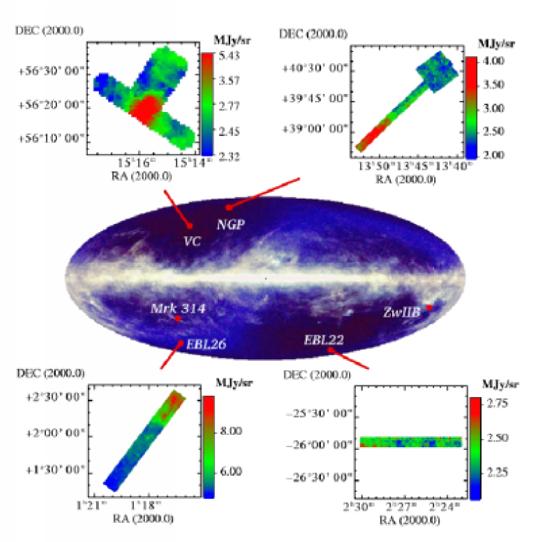
Figure 1: The positions of the observed FIR fields overlaid on the all-sky map composed of the DIRBE 60, 100, 140 and 240$\mu$m Annual Average Sky Maps. The 180$\mu$m ISOPHOT maps are shown for four regions. Besides dark areas the fields contain, on purpose, also areas with faint cirrus

3 The point source detection

The point source detection was performed in two steps using data processed to the AAP level with PIA and the pairwise method (see Sect. 2). The data consists of surface brightness values with error estimates and were flat fielded using special routines (see Appendix B.1).

In the first phase each surface brightness value was compared with the mean and the standard deviation estimated from other measurements within a fixed radius. The radius was set to about three times the size of the detector pixel. Values rising above the local mean surface brightness by more than 0.7$\sigma$ were considered as potential point sources.

In the second phase a model consisting of point source and a constant background was fitted into each region surrounding the candidate positions. In the fit the footprint matrices were used to calculate the contribution of the point source to the observed surface brightness values. The free parameters of the fit were the source flux density, the two coordinates of the source position, and the background surface brightness. Details of the fitting procedure are given in Appendix B.2

3.1 Completeness and false detections

As a result of the fitting procedure we obtained estimates for the flux density, coordinates of the potential point source and a value for the local background brightness. The fitting routine provides formal error estimates for all free parameters. In addition, we have calculated the standard deviation of the surface brightness values inside the selected region. Assuming that the flux density values are normally distributed we can calculate for each source candidate the probability, $P$, that the detection is not caused by background noise.

The completeness of the point source detection and the probability of false detections were studied with simulations (see Appendix B.3). The number of false sources was found to somewhat exceed the expected number of 1-$P$ per map pixel and this was taken into account in setting the selection criteria. A confidence limit of $P$=99% (corresponding to $\sim$2.3 $\sigma$) was used to discard uncertain detections.

Simulated measurements were also used to study the effects of imperfect flat fielding (Appendix B.4). These do not cause significant errors in the source counts. Cosmic ray glitches and short term detector drifts may still lead to spurious detections primarily on the C100 detector. Glitches have been removed during the standard data reduction and any remaining anomalies should be reflected in the error estimates calculated for the surface brightness values. Large error estimates will reduce the number of false detections (see C).

For the purpose of source counts (see Sect. 5.1) we will use an additional criterion based on the ratio between the source flux density, $S_{\nu}$, given in Jy and the background rms noise, $\sigma_{\rm bg}$, given in units of Jy per pixel,

$$\rho=\frac{S_{\nu}}{\sigma_{\rm bg}}.$$ (1)

The parameter $\rho$ is not directly related to the probability obtained from the footprint fit and can be used as safeguard against false detections. In Sect. 5.1 we will use a limit $\rho>\rho_{\rm 0}=$10.5. In the maps fluctuations are typically below 0.1 MJy sr^-1 which, in the case of the C200 detector, corresponds to $\sigma_{\rm bg}\sim$0.02 Jy per pixel. Our $\rho$-criterion implies thus a typical detection limit of 200 mJy. Because of the smaller pixel size of the C100 detector, $\sim$44$\arcsec$ instead of $\sim$89$\arcsec$, the detection limit is lower by a factor of four. Note that since the source flux is always distributed over several map pixels $\rho$ cannot be interpreted directly as a $\sigma$ limit.

The value $\rho_{\rm 0}=$10.5 was chosen based on simulations: at this limit the detection rate is $\sim$70% for sources which fulfill the previous criterion of $P>$99%. The number of false detections is less than one per 200 map pixels. For the C200 detector the expected number of false detections within the mapped areas is $\la$10 i.e. less than the probable number of true sources above the $\rho$ limit that remain undetected. Because of the larger number of map pixels in the 90$\mu$m maps there can be more false detections than undetected true sources. However, the relative error in the source counts should remain well below 50%.

3.2 Multiwavelength confirmation of source detections

Since the source counts might be slightly overestimated even after applying the additional $\rho$-criterion constraint we have constructed another source list based on multi-wavelength detections. A source is accepted only if there are detections at two wavelengths, each at 99% confidence level (see above), and the spatial distance between these detections is $\leq$80$\arcsec$. The $\rho$ criterion is not used. If a map contains several possible sources within that distance the one with the highest estimated probability is selected. With the number density of detections at the 99% confidence level we can estimate the probability of finding by accident a source within 80$\arcsec$ radius of any given position: 5% for the 90$\mu$m and 150$\mu$m maps and below 10% even for 180$\mu$m.

We can calculate a rough estimate for the number of false detections as follows. For any individual detection we have an 1% probability that it is not caused by a real source. Empirically, the probability of finding another detection at a different wavelength within 80$\arcsec$ radius is less than 10%. This increases the confidence in the first detection from 99% to 99.9%. In the source counts for 150$\mu$m and 180$\mu$m the total number of spurious detections can therefore be estimated to be $\sim$1. Because of the larger number of pixels in the 90$\mu$m maps the number of false 90$\mu$m sources could be up to $\sim$6. However, the false detections are made only close to the background noise level where the number of undetected true sources can easily exceed this. Counting only detections with multiwavelength confirmation will underestimate the true number of sources. The probability of finding two spurious detections within 80$\arcsec$ is 0.001% and the confidence level of a source detected at two wavelengths (instead of a detection at one wavelength only) equals a 4.2$\sigma$ detection.

Examples of such multiwavelength detections are shown in Fig. 2. The positions of four sources in the field EBL26 are overlaid on the 90$\mu$m, 150$\mu$m and 180$\mu$m maps. Sources 5 and 6 are detected only at 150 and 180 $\mu$m (see also Table 5.1). The leftmost source is a 90$\mu$m detection only and is therefore not in Table 5.1. It is probably caused by a glitch as can be seen from the SRD data (Signal per Ramp Data i.e. signals, V s^-1, derived from individual detector integration ramps) in Fig. 3a. The signals are shown for four pixels at five positions (given as a function of time) centered on the position closest to the fitted source position. Source 7 was detected only at 150$\mu$m and 180$\mu$m while at 90$\mu$m it remained below our detection limit. The SRD data for this source are also shown in Fig. 3. One must remember that the detection procedure was not based on SRD data and in Fig. 3 only part of the relevant data are shown. SRD signals were, however, used to visually estimate the possible effect of glitches on the source detections (see C).

Figure 2: The positions of four detections in EBL26 overlaid on the 90$\mu$m, 150$\mu$m and 180$\mu$m maps. The leftmost source was detected only at 90$\mu$m while the other sources (numbers 5, 6 and 7) were detected at 150$\mu$m and 180$\mu$m. See Table 5.1 for parameters of the numbered sources

Figure 3: SRD signals for two sources shown in Fig. 2: a source detected at 90$\mu$m only (a) and the Source number 7 (b). The signals are shown for four pixels as function of time for five consecutive raster positions. For each pixel the plot is centered on the position closest to the average positions of the detections made at different wavelengths. The signals from this position are between the dashed lines. The pixel numbers are shown in the figure. The first source was detected at 90 $\mu$m only while the second one was detected at 150$\mu$m and at 180$\mu$m

For most of the area of the 15$\times$15 position 180$\mu$m map NGPN no observations at other wavelengths were available. In order to confirm the detections the data were divided at the ERD level into two parts. The first data set contained the first ramps of each measurement and the second data set the rest of the ramps. These data sets were used to create two maps and sources were detected and accepted according to procedures described above. The maps are not completely independent. A large glitch that affects several ramps may have influenced both data sets. The risk for false detections is therefore larger than in other cases. Some of the detections could, however, be confirmed with observations of the 32$\times$4 position NGPN map which partly overlaps the square 15$\times$15 position 180$\mu$m map (see Table 1).

4 Discrimination against cirrus knots

We will check the possibility that some of the sources detected are small scale cirrus structures (cirrus knots).

4.1 Cirrus confusion noise

We estimate the contribution of cirrus to the sky confusion. The total noise, $\sigma_{\rm total}$, in the source flux densities is estimated from the standard deviation of the flux densities. This is obtained by fitting a point source to the position of each measurement (each pixel and raster position) while keeping the source positions fixed i.e. effectively convolving the map with the detector footprint. The total noise consists of measurement noise, $\sigma_{\rm meas.}$, from the detector, and the sky confusion, $\sigma_{\rm sky}$, caused by real sky brightness variations,

$$\sigma_{\rm total}^{2}=\sigma_{\rm meas.}^{2}+\sigma_{\rm sky}^{2}.$$ (2)

The measurement noise, in flux density units, is derived from the error estimates obtained for the surface brightness values from the SRD data. The surface brightness map was modified by adding corresponding amount of normally distributed noise. The fitting procedure was then repeated. The rms difference between the flux densities obtained from the two maps gives an estimate of measurement errors on the flux density scale. Table 2 summarizes the results for the fields EBL26 and NGPS. The sky confusion is obtained (using Eq.2) from the total and measurement noise estimates. The measurement noise was seen to be roughly equal to the sky confusion. In order to estimate the contribution of cirrus to the sky noise we have used the approach of Gautier et al (gautier92 (1992)).

Table 2: The estimated total rms noise, $\sigma_{\rm total}$, in the fields EBL26 and NGPS compared with the estimated measurement noise, $\sigma_{\rm meas.}$, and the sky confusion, $\sigma_{\rm sky}$

field	$\lambda$	$\sigma_{\rm total}$	$\sigma_{meas.}$	$\sigma_{\rm sky}$
	($\mu$m)	(mJy)	(mJy)	(mJy)
EBL26	90	41	32	25
	150	117	55	104
	180	110	56	88
NGPS	90	29	24	17
	150	51	36	36
	180	57	41	40

Gautier et al. (gautier92 (1992)) calculated the confusion noise due to infrared cirrus for different observation strategies. We use these results to estimate cirrus contamination in the case of circular aperture with diameter $d$, immediately surrounded by a reference annulus of the same width. This configuration is not exactly the same as in our detection procedure but should give accurate estimates of the expected cirrus confusion.

Herbstmeier et al. (herbstmeier (1998)) estimated for the large NGPN 180$\mu$m map a fluctuation power $P=$2.3$\times$10³ Jy² sr^-1 at the scale of 4$\arcmin$. The fluctuations are mostly due to cirrus emission. With the dependence $P\sim d^{2}$ derived by Herbstmeier et al. we obtain a fluctuation amplitude of 18 Jy sr^-0.5 at $d=$1.5$\arcmin$ which corresponds to the size of the detector beam. According to the tables of Gautier et al. (gautier92 (1992)) the estimated flux density fluctuations due to cirrus emission are 8.0 mJy. In this field all detected sources have flux densities exceeding 100 mJy. It is therefore very unlikely that they could be caused by cirrus.

The surface brightness attributed to cirrus is obtained by subtracting the CIRB given by Fixsen et al. (fixsen98 (1998)), 0.82 MJy sr^-1 at 180$\mu$m, and the zodiacal light according to Leinert et al. (leinert98 (1998)). In the field, EBL26, which has the largest surface brightness among our fields, the average cirrus surface brightness is $\sim$1.4 MJy sr^-1 compared to $\sim$0.8 MJy sr^-1 in the NGPN field. With the relation $P\sim<B>^{3}$ (Gautier et al. gautier92 (1992)) between the fluctuation power and the mean surface brightness we can estimate that in EBL26 the cirrus fluctuation level is $\sim$43 mJy. All sources are above $\sim$150 mJy, i.e. above the 3.5 $\sigma$ level.

The results of Herbstmeier et al. (herbstmeier (1998)) show that at the scale of the C100 beam size, $d\sim 45\arcsec$, the expected cirrus fluctuation amplitude is clearly below 10 Jy sr^-0.5 for all our 90$\mu$m maps. According to Gautier et al. (gautier92 (1992)) this corresponds to a flux density of 4 mJy which is again clearly below the flux densities of even the faintest sources at 90 $\mu$m in the present study.

In conclusion, it is clear that cirrus is not the dominant factor in the sky confusion noise. The flux density values derived for cirrus contamination are small compared with the faintest sources detected here. Because of the non-gaussian nature of the cirrus fluctuations (Gautier et al. gautier92 (1992)) it is, however, possible that our source lists contain some cirrus knots.

We have, however, also the advantage of having observations at different wavelengths which offers an additional means for the discrimination against spurious detections caused by galactic cirrus.

4.2 Cirrus spectra

Using observations made at different wavelengths we can determine the cirrus spectrum in each region. For each 180$\mu$m measurement the corresponding surface brightness values at the other wavelengths were calculated using weighting with a gaussian with the approximate size of the C200 detector beam. Linear fits were performed to surface brightness values at 90$\mu$m or 150$\mu$m plotted against the 180$\mu$m values and the slopes were used to derive the cirrus spectrum (see Juvela et al. vilspa (2000)).

The spectra obtained are shown in Figs. 4-7. The cirrus spectrum can be determined most reliably in regions with clear surface brightness variations which is the case for fields EBL26 and NGPS. It is also, nevertheless, possible to determine the spectra for all other fields. Bright individual sources were always removed from the data but in the VCS and VCN fields the results may be influenced by the emission from the nearby galaxy, NGC 5907.

4.3 Source spectra vs. cirrus spectra

The cirrus spectra were compared with the spectra of the detected sources. The relationship between the cirrus surface brightness spectrum and the “source” spectrum due to a cirrus knot depends on the size of the cirrus knot: (1) If the cirrus knot is small compared with the C100 detector pixel, the knot spectrum is the same as the surface brightness spectrum. (2) If the knot size is $>$45$\arcsec$ some part of the 90$\mu$m flux is included into the background, and the source flux density at 90$\mu$m drops. (3) If the cirrus knot is large compared even with the pixel size of the C200 detector also at the longer wavelengths only part of the total flux density contained in the cirrus knot will be detected. In that case there will be probably no detection with the C100 detector.

Simulations showed that for gaussian cirrus knots with FWHM $\sim$90$\arcsec$ we detect with the C100 detector less than half of the total flux density. For cirrus knots with FWHM$\sim$180$\arcsec$ the ratios $F(90\mu$m)/$F(150\mu$m) and $F(90\mu$m)/$F(180\mu$m) drop to $\la$0.25 of the cirrus surface brightness values.

If the source spectrum is flat compared to the cirrus surface brightness spectrum we can conclude the source is not a cirrus knot. Otherwise, this alternative cannot be excluded with certainty. However, when the flux density ratio $F(90\mu$m)/$F(150\mu$m) or $F(90\mu$m)/$F(180\mu$m) is clearly larger than one fourth of the corresponding ratio in the cirrus surface brightness spectrum it is improbable that the source is due to a cirrus knot because this would require that the knot is much smaller than 180$\arcsec$. From the slope of the cirrus power spectrum as function of spatial frequency, (Gautier et al. gautier92 (1992); Low & Cutri low (1994); Herbstmeier et al. herbstmeier (1998)) and the very low level of cirrus emission in most of the fields, we estimate that it is very improbable that there are many small ($\la$90$\arcsec$) cirrus knots strong enough to be detected as sources (see Sect. 4.1).

In Figs. 4-7 we show for our four main fields the predicted spectra caused by cirrus knots together with those actual sources that were detected at 90$\mu$m and at some longer wavelength. The cirrus spectra have been drawn for two cases assuming either that the cirrus knot is smaller than the C100 detector pixel (solid line) or that it is of the same size as the beam of the C200 detector pixels (dashed line).

The source spectra are almost without exception flat compared with the steeper of the two cirrus spectra and the sources are not likely to be caused by cirrus. Furthermore, in many cases the relative 90$\mu$m flux is higher than what is possible even for very small cirrus knots. No sources were rejected from our sample based on their SED shape.

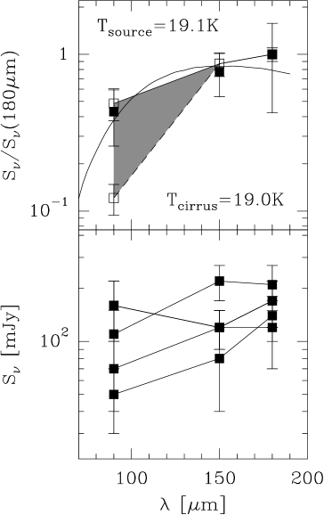
Figure 4: Average source spectrum of the fields VCN and VCS (filled squares) and the cirrus spectrum determined in the same fields (open squares). The shaded area indicates the possible range for cirrus spectra. At 90$\mu$m the highest cirrus flux is obtained when the knot is small compared with the C100 pixel size and the lowest flux density corresponds to a knot with size similar to the C200 detector pixels. The upper cirrus spectrum and the average source spectrum have been fitted with modified Planck Law, $\nu^{2}B_{\nu}$, with temperatures shown in the figure (upper frame). Spectra of sources in fields VCN and VCS detected at 90$\mu$m and at one or two longer wavelengths. The average source spectrum has been calculated without including the source with the highest 90$\mu$m flux density (lower frame)

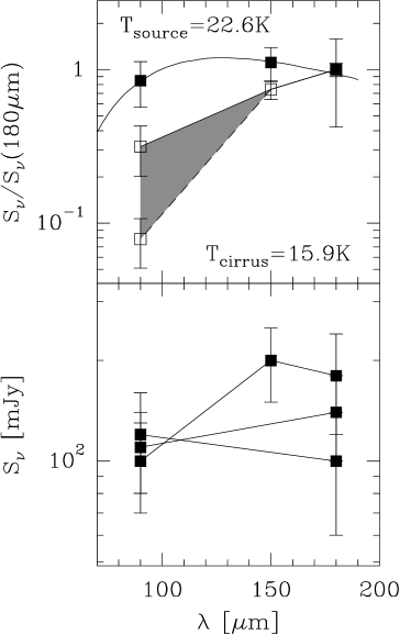
Figure 5: Cirrus spectrum and source spectra in the field EBL22 (symbols as in Fig. 4

Figure 6: Cirrus spectrum and source spectra in the field EBL26 (symbols as in Fig. 4

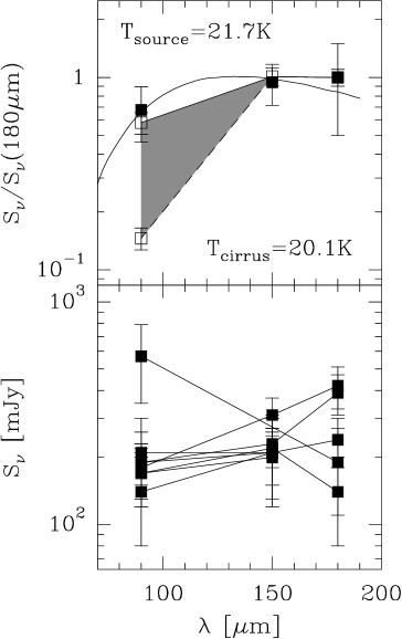
Figure 7: Cirrus spectrum and source spectra combined from the fields NGPN and NGPS (symbols as in Fig. 4. The plotted average source spectrum has been calculated without including the source with the highest 90$\mu$m flux

Figure 8: Cumulative source counts at 90$\mu$m, 150 $\mu$m and 180$\mu$m. The solid and the dotted lines represent values obtained by estimating the areas according to the faintest sources detected in a map. The dotted line gives all sources detected and the solid line sources detected at more than one wavelength. The dashed curves represent cases in which both the the source selection and the area determination were based on the local background variations (see Sect. 5.1). The Poisson noise of the count statistics is indicated at some representative points with vertical error bars

5 Source counts and identifications

5.1 Cumulative source counts

Table 5.1 contains sources detected at two or three wavelengths with an individual detection probability $P>$99% at one wavelength (see Sect. 3.2). The coordinates are averages, weighted with the estimated confidence of detections at different wavelengths. The flux densities and their error estimates are obtained from the fitting routine. If the field was mapped at three wavelengths but the source was detected only at two wavelengths, then we quote an upper limit based on the background surface brightness variations, $S=10.5\sigma_{\rm bg}$ where $\sigma_{\rm bg}$ is given in units of Jy per pixel. The detection probability corresponding to this limit is 97%.

Table 3: (See next page) Sources detected at two or more wavelengths. The coordinates are weighted averages of the positions fitted at different wavelengths. For sources undetected at one wavelength we give upper limits which, according to simulations, correspond to the flux density of a source with detection probability 97%. Quality flags, $q$, are based on visual inspection of the SRD data and the scale is from 0 (obvious glitch) to 4 (clear source). Counts $c$ are the results from our detection procedure based on the SRD data (see C). Asterisks mark cases where a detection at one wavelength could be associated with two different detections at another wavelenth. The confidence level of each detection at one wavelength is 99% while the confidence level for a source with two detections at different wavelengths is better than 99.99%

				90$\mu$m		120$\mu$m		150$\mu$m		180$\mu$m
Field	Source No.	R.A.	Dec	$S$	$q/c$	$S$	$q/c$	$S$	$q/c$	$S$	$q/c$
(2000.0)	(2000.0)	(Jy)		(Jy)		(Jy)		(Jy)
EBL22	1	02 24 27.2	-25 55 11	$<$0.10		-		0.12(0.04)	3/7	0.15(0.05)	4/10
	2	02 24 33.6	-25 50 18	$<$0.07		-		0.23(0.03)	4/10	0.21(0.05)	4/10
	3	02 25 28.0	-25 56 34	$<$0.07		-		0.21(0.05)	3/10	0.27(0.05)	4/10
	4	02 26 58.4	-25 50 49	0.12(0.04)	3/19	-		$<$0.13		0.10(0.04)	2/2
	5	02 28 19.7	-25 56 55	0.10(0.03)	2/16	-		0.20(0.05)	3/4	0.18(0.06)	2/6
	6	02 28 44.8	-25 50 31	0.11(0.03)	1/15	-		$<$0.14		0.14(0.04)	3/8
EBL26	1∗	01 16 38.9	+02 30 45	0.36(0.06)	1/4	-		0.85(0.19)	4/9	1.05(0.21)	4/7
	2∗	01 16 40.3	+02 30 01	0.36(0.06)	1/4	-		0.87(0.30)	4/8	0.92(0.29)	4/7
	3∗	01 17 09.2	+02 16 45	2.64(1.03)	4/20	-		1.82(0.33)	4/10	1.68(0.37)	4/8
	4∗	01 17 09.3	+02 17 13	2.64(1.03)	4/20	-		1.82(0.33)	4/10	1.71(0.44)	4/8
	5	01 17 49.7	+02 00 29	$<$0.14		-		0.33(0.13)	4/10	0.36(0.10)	3/9
	6	01 17 53.5	+02 09 25	$<$0.22		-		0.48(0.14)	4/10	0.34(0.10)	3/9
	7	01 18 03.8	+01 59 09	$<$0.13		-		0.85(0.14)	4/10	0.56(0.08)	4/10
	8	01 18 34.6	+01 45 07	$<$0.16		-		1.04(0.10)	4/10	0.59(0.11)	3/10
	9	01 19 07.5	+01 31 15	0.14(0.05)	2/14	-		$<$0.26		0.16(0.05)	2/5
Mrk 314	1	23 02 52.3	+16 31 52	-		0.20(0.06)	1/4	-		0.32(0.11)	3/8
	21	23 02 59.7	+16 36 10	-		1.32(0.17)	2/7	-		0.91(0.17)	4/10
	3	23 03 30.6	+16 36 11	-		1.09(0.16)	2/2	-		1.09(0.19)	2/4
NGP	1	13 41 22.8	+40 41 54	$<$0.17		-		0.49(0.06)	2/6	0.50(0.06)	3/6
	2	13 42 03.1	+40 28 13	$<$0.09		-		0.31(0.06)	3/7	0.27(0.05)	3/6
	3	13 42 22.1	+40 21 58	0.17(0.05)	3/11	-		0.20(0.07)	2/0	$<$0.30
	4	13 42 41.7	+40 27 12	$<$0.13		-		0.23(0.05)	3/5	0.29(0.07)	2/6
	5	13 42 46.9	+40 18 02	$<$0.14		-		0.30(0.08)	2/8	0.45(0.10)	3/8
	6	13 43 03.3	+40 14 51	0.19(0.07)	3/15	-		0.23(0.08)	2/0	0.39(0.08)	2/1
	7∗	13 43 39.8	+40 13 56	0.14(0.06)	3/14	-		0.21(0.06)	3/5	0.24(0.06)	3/10
	8∗	13 43 41.5	+40 14 02	$<$0.13		-		0.21(0.06)	3/5	0.24(0.06)	3/10
	9	13 43 46.7	+40 07 54	$<$0.11		-		0.14(0.06)	1/0	0.20(0.07)	2/0
	10	13 45 03.2	+39 55 04	$<$0.13		-		0.18(0.06)	4/10	0.25(0.10)	4/10
	11	13 45 44.6	+39 47 17	$<$0.10		-		0.13(0.05)	4/9	0.21(0.08)	4/10
	12∗	13 47 17.3	+39 36 50	0.19(0.04)	3/13	-		0.21(0.09)	2/3	$<$0.23
	13∗	13 47 19.0	+39 37 00	0.21(0.09)	3/10	-		0.21(0.09)	2/3	$<$0.26
	14	13 47 33.8	+39 32 04	$<$0.15		-		0.19(0.05)	3/1	0.22(0.09)	2/0
	15	13 48 24.0	+39 21 23	$<$0.13		-		0.16(0.05)	2/1	0.16(0.04)	2/0
	16∗	13 48 30.4	+39 27 12	$<$0.11		-		0.22(0.04)	3/4	0.14(0.06)	3/8
	17∗	13 48 31.9	+39 26 58	0.17(0.04)	1/4	-		0.22(0.04)	3/4	0.14(0.06)	3/8
	18	13 49 07.6	+39 16 54	0.18(0.05)	2/12	-		0.31(0.06)	3/6	0.42(0.09)	3/2
	19	13 49 31.5	+39 04 55	0.57(0.22)	3/16	-		$<$0.20		0.19(0.08)	2/0
	20	13 49 36.1	+39 07 11	$<$0.15		-		0.15(0.06)	3/6	0.20(0.08)	2/3
	21	13 50 35.8	+39 00 29	$<$0.14		-		0.21(0.08)	2/1	0.26(0.09)	2/3
	22	13 50 56.2	+38 58 18	$<$0.12		-		0.32(0.11)	2/2	0.42(0.11)	3/4
	23	13 52 14.1	+38 39 35	$<$0.11		-		0.17(0.06)	3/6	0.21(0.07)	2/0
	24	13 52 33.1	+38 42 33	$<$0.13		-		0.26(0.06)	4/8	0.28(0.08)	3/10
	25	13 52 51.6	+38 39 00	$<$0.11		-		0.36(0.06)	2/3	0.27(0.09)	3/8
VCN, VCS	1	15 15 14.5	+56 29 36	$<$0.10		-		0.10(0.03)	2/5	0.10(0.03)	3/2
	2	15 15 20.8	+56 30 43	$<$0.10		-		0.08(0.03)	2/0	0.15(0.03)	2/0
	3	15 15 26.3	+56 32 06	$<$0.10		-		0.13(0.04)	2/3	0.11(0.03)	2/1
	4	15 14 28.3	+56 10 26	$<$0.09		-		0.16(0.04)	3/1	0.19(0.04)	2/0
	5	15 14 38.7	+56 34 06	0.11(0.04)	3/5	-		0.22(0.05)	2/0	0.21(0.06)	2/0
	6∗	15 16 48.0	+56 26 15	0.07(0.03)	2/1	-		0.12(0.03)	2/2	0.17(0.05)	2/0
	7∗	15 16 49.1	+56 26 23	0.16(0.06)	2/1	-		0.12(0.03)	2/2	0.17(0.05)	2/0
	8∗	15 16 50.7	+56 26 18	0.16(0.06)	2/1	-		0.12(0.03)	2/2	0.12(0.05)	2/0
	92	15 15 54.3	+56 19 26	19.02(2.70)	3/14	-		34.94(3.69)	3/4	37.99(4.27)	4/10
	10	15 14 56.7	+56 35 21	0.05(0.02)	2/0	-		0.08(0.04)	2/3	0.14(0.04)	2/0
ZW IIb	13	05 10 48.4	-02 40 45	-		0.55(0.12)	2/0	-		0.62(0.21)	3/2
	2	05 10 56.2	-02 45 41	-		0.38(0.13)	2/2	-		0.52(0.18)	2/0

¹ Mrk 314 ² NGC 5907 (see Sect. 5.3) ³ Zw II b

The surface density of sources is estimated by dividing the number of sources counted at each flux density level by the total effective map area. With “effective” map area we mean that portion of the total map area from which such sources could have been detected. For example, in the field VCN faint sources cannot be detected close to the bright galaxy NGC 5907. The maps around Mrk 314 and ZW IIB were originally observed in order to study a known object and since these bright sources are not the result of random selection they are excluded from the source counts.

As a first approximation we have calculated the effective map areas according to the faintest detected source. At each flux density level the area was taken to be the sum of the areas of those maps where sources with equal or lower flux densities were detected. The procedure is likely to underestimate the surface density of faint sources since it ignores the background surface brightness variations within the maps. The detection of just one source with a flux density $S_{\nu}$ increases the corresponding area $A(S_{\nu})$ by the the area of the whole map. On the other hand, for statistical reasons the faintest detected source can sometimes be brighter than the faintest theoretically detectable source but this should not lead to significant underestimation of the areas at any flux density levels.

For 90$\mu$m maps observed with a 180$\arcsec$ raster step there are gaps between the rasters. We have chosen not to correct for this effect but note that it may lead to an underestimate of the source densities by some tens of per cents i.e. the effect is comparable with the calibration uncertainties.

The cumulative source densities obtained at 90$\mu$m, 150$\mu$m and 180$\mu$m are shown as histograms in Fig. 8. Two sets of sources were used in deriving these curves. The first set consists of all detections (i.e. $P>$99%) and no confirmation was required at a different wavelength (dotted line). The second set contains only those sources that were confirmed by a detection at another wavelength (solid line).

The first set may contain a number of false detections. The second set gives a conservative estimate for the true number of sources. Since the areas used in deriving the surface densities depend also on the selection criteria applied, the sample with the larger number of sources does not necessarily lead to higher source density. The results obtained from the two sets are very similar for 150 and 180$\mu$m. At 90$\mu$m the counts based on detections confirmed at 150$\mu$m or 180$\mu$m are, however, below the other estimates. Most of the difference can be explained by statistical uncertainties. There are only three confirmed 90$\mu$m sources brighter than 400 mJy and at lower flux levels where the number of sources is larger the estimates are in fair agreement with each other. The change in the ratio between the two estimates as the function of source flux is not statistically significant. Some of the difference may be caused also by the source properties. Sources detected at 150$\mu$m are likely to be seen also at 180$\mu$m (and vice versa) while more of the 90$\mu$m sources remain unconfirmed at the longer wavelengths.

We have derived a third set of cumulative source densities by selecting sources based on the ratio $\rho$ between the flux density and the background surface brightness variations (see Sect. 3.1). For each flux density level all sources with $\rho>\rho_{0}$ were selected and no confirmation at other wavelengths was required. The area corresponding to a given flux density level was obtained by first calculating the local standard deviation of the surface brightness values around each observed position and then integrating the total area with noise below 1/$\rho_{0}$ times the source flux density.

The limiting value, $\rho_{0}=$10.5, was selected based on simulations (see Sect. 3.1) which indicate that close to the detection limit the number of false detections is still clearly less than the expected number of true sources. In the measurements the typical background noise is 0.02 Jy per pixel and the given $\rho$ value corresponds to source flux density limits 45 mJy and 200 mJy for C100 and C200, respectively. For higher flux densities the number of false detections drops rapidly while for lower flux densities more of the true sources are either rejected based on the $\rho$ criterion or are not detected at all. At the quoted flux levels the cumulative source counts are higher than the number of the false detections which will therefore not affect the results significantly. However, especially at 90$\mu$m, the number of false detections can exceed the number of undetected true sources and the source counts could be slightly overestimated.

The cumulative source densities obtained with this third method are drawn in Fig 8 with dashed lines. These results are based on the integrated area of the regions where background noise is low enough for a source with given flux density to be detectable. Since the area determination and the source detection are based on similar criteria the errors caused by an incorrect $\rho$–limit tend to cancel out. At the bright end the results agree with the earlier histograms since no sources are rejected and the corresponding areas converge towards the total area mapped. The differences are more pronounced at faint flux densities. When the area corresponding to a faint flux density limit was determined based on the faintest observed source the area was likely to be overestimated and the source densities underestimated. When the area was determined by the local properties of the background brightness and the sources were selected using a related criterion the results should be more reliable. On the other hand, the applied $\rho$ limit excludes many of the fainter (but more uncertain) sources that were included in the previous counts and the curves cannot be extended reliably to equally low flux densities. The values obtained for 150$\mu$m and 180$\mu$m below 150 mJy are probably only indicative.

5.2 Cumulative flux densities

Fig. 9 shows the cumulative flux densities, $F_{\nu}(S_{\nu})$, i.e. the surface brightnesses due to all sources brighter than a given flux density $S_{\nu}$. Compared with source counts the flux density values are more sensitive to bright sources.

Systematic calibration errors would cause the curves to be shifted horizontally. Our simulations show that the source flux densities depend also on the detection process. The fitted source positions can be slightly displaced from the true positions towards a direction where the background noise produces the highest values. Therefore it is possible that the faintest flux densities are overestimated. The errors are, however, only noticeable close to the detection limit and should never be more than 10%. Furthermore, several maps were observed with partly overlapping rasters. The improved sampling should lead to more reliable flux densities. The largest uncertainty is therefore in the absolute calibration itself.

Figure 9: Cumulative flux densities, $F_{\nu}$, at 90$\mu$, 150 $\mu$m and 180$\mu$m in units of surface brightness. The curves correspond to samples obtained with the same methods as in Fig. 8

5.3 Association with known sources

Table 4 lists IRAS Point Source Catalog (PSC) and Faint Source Catalog (FSC) sources within the mapped regions. ISOPHOT sources detected within a $\sim$1$\arcmin$ radius of the IRAS positions are also shown.

In the regions studied there are four sources with IRAS detections at 100$\mu$m. In EBL26 the PSC source at 1^h17^m10.6^s +2$\degr$17$\arcmin$10$\arcsec$ has been detected also with ISOPHOT. The flux density obtained at 90$\mu$m, 2.6 Jy, is somewhat higher than the IRAS 100$\mu$m value of 2.2 Jy. The FSC source at 1^h18^m05.0^s +1$\degr$58$\arcmin$59$\arcsec$ with 0.84 Jy flux density at 100$\mu$m has not been detected and the quoted 90$\mu$m upper limit is 110 mJy. The reason is that the 90$\mu$m map was incompletely sampled and the IRAS position lies between the observed rasters.

In VCS the IRAS source at 15^h15^m53.3^s +56$\degr$19$\arcmin$47$\arcsec$ is the bright galaxy NGC 5907. The source is extended and the ISOPHOT map is too narrow for the estimation of the total flux density. The ISOPHOT values in Table 4 are obtained by fitting of a point source within an area with 5$\arcmin$ radius. The flux density at 90$\mu$m is slightly lower than the IRAS value. In the case of Mrk 314 the flux densities at 120$\mu$m are comparable to the IRAS 100$\mu$m values. There are additionally a number of IRAS sources with upper limits at 100$\mu$m. In all cases the ISOPHOT upper limits derived at 90$\mu$m are much lower although in the case of maps observed with 180$\arcsec$ raster steps the upper limits are not always accurate.

Table 4: IRAS Faint Source Catalog and Point Source Catalog sources within a $\sim$1$\arcmin$ radius of the positions listed in Table 5.1

In Table 5 we list objects from the Simbad database that are within the mapped regions. The list contains all sources identified as galaxies or quasars. Other types of objects (e.g. radio sources) are listed only if they are close to a FIR detection.

Table 5: Sources from the Simbad database together with FIR detections within $\sim$1.5$\arcmin$ radius. The table contains all galaxies and QSOs inside the regions mapped and all other objects close to sources detected in the ISOPHOT maps

6 Discussion

6.1 Comparison with other ISOPHOT source counts

At the flux level of 100 mJy the following source densities are obtained (dotted line in Fig. 8): 1.4$\times$10⁵ sr^-1, 2.5$\times$10⁵ sr^-1 and 3.5$\times$10⁵ sr^-1 at 90 $\mu$m, 150 $\mu$m and 180 $\mu$m. In Fig.10 these results are compared with results from other ISOPHOT projects.

At 90$\mu$m the results of Kawara et al. (kawara (1998)) are some 30% higher than our source counts while the results of the ELAIS survey (Oliver et al. ringberg (2000)) and Linden-Vørnle et al. (linden (2000)) are lower than our counts. The ELAIS counts based on observations of 11.6 square degrees at 90$\mu$m, are a factor of three below the Kawara et al. (kawara (1998)) value.

The calibration adopted in the ELAIS project is based on DIRBE and it was found that the PIA analysis resulted in higher surface brightnesses (Efstathiou et al. efstathiou00 (2000)). This is consistent with our findings. The difference between the DIRBE surface brightness values and our data calibrated with PIA version 7.3 is $\sim$30% (A). With DIRBE calibration our source count points at 90$\mu$m move towards smaller flux densities (see Fig. 10) and they would be in good agreement with the ELAIS results.

At 180$\mu$m we can compare our source counts with Kawara et al. (kawara (1998)) and Puget et al. (puget99 (1999)) observations at 175$\mu$m. Our counts are almost two times higher than the Kawara et al. results but compatible with Puget et al. (puget99 (1999)).

6.2 Comparison with galaxy models

At 150$\mu$m and 180$\mu$m the counts are much higher than predicted by no-evolution models (e.g. Guiderdoni et al. guiderdoni98 (1998)); at 180 $\mu$m the difference is a factor of five (see Fig. 10).

In the evolutionary model E by Guiderdoni et al. (guiderdoni98 (1998)) both the star formation rate and the relative number of ULIRGs increase with $z$. The model has been found to be in good agreement with extragalactic background light measurements in both optical and FIR. Our source counts exceed, however, the model predictions at all three wavelengths (see Fig. 10).

Franceschini et al. (franceschini98 (1998)) have presented similar models which include contributions from two galaxy populations: dust-enshrouded formation of early-type galaxies and late-type galaxies with enhanced star-formation at lower redshifts. The predicted source counts at 180$\mu$m are higher than in the Guiderdoni et al. model E and the model is therefore in better agreement with our results.

Figure 10: Comparison with other ISOPHOT counts and models of galaxy evolution. Our source counts at 100 mJy and 200 mJy are shown together with the results of Puget et al. (puget99 (1999); circles), Kawara et al. (kawara (1998); triangles), Oliver et al. (ringberg (2000); diamonds) and Linden-Vørnle (linden (2000); stars). We present our results as horizontal lines that indicate the difference between the DIRBE calibration and the adopted ISOPHOT calibration. At 90$\mu$m the DIRBE calibration results in lower flux densities and at 150$\mu$m and 180$\mu$m in higher flux densities. The predictions of model E of Guiderdoni et al. guiderdoni98 (1998) are shown with solid lines and the evolutionary model of Franceschini et al. franceschini98 (1998) with a dashed line. Dotted lines show predictions of no-evolution models (90$\mu$m: Guiderdoni et al. guiderdoni98 (1998); 150$\mu$m and 180$\mu$m: Franceschini et al. franceschini98 (1998))

6.3 Extragalactic background radiation

Measurements of the CIRB in the wavelength range of the present observations have been recently published based on DIRBE and FIRAS observations of the COBE satellite. After the removal of interplanetary and galactic foreground sources (Kelsall et al. kelsall (1998); Arendt et al. arendt (1998)) the level of CIRB detected by DIRBE was found to be 25$\pm$7 nW m^-2 sr^-1 at 140 $\mu$m and 14$\pm$3 nW m^-2 sr^-1 at 240 $\mu$m (Hauser et al. hauser (1998)). These numbers correspond to 1.1 MJy sr^-1. According to Fig. 9 the sources found in this study represent some 5% of the CIRB, the exact number depending on which source counts are applied.

Fixsen et al. (fixsen98 (1998)) have reported results based on three different methods used to subtract the galactic foreground emission. From the analytical representation of the average spectrum the surface brightness values at 90 $\mu$m, 150 $\mu$m and 180$\mu$m are 0.13 MJy sr^-1, 0.67 MJy sr^-1 and 0.82 MJy sr^-1, respectively. Adopting these values our sources would contribute already a significant fraction of the CIRB, especially at 90$\mu$m where $\ga$20% of the CIRB could be attributed to the detected sources. For sources brighter than 100 mJy the corresponding fraction at 150 $\mu$m is slightly below and at 180$\mu$m slightly above 10%. Recalibrating the 140$\mu$m and 240$\mu$m DIRBE observations using the results of the cross-calibration between FIRAS and DIRBE (Fixsen et al. fixsen97 (1998)) would, naturally, move the DIRBE points closer to the FIRAS values (Fixsen et al. fixsen98 (1998)). As discussed in A, our calibration appears to be closer to the FIRAS than the DIRBE scale.

6.4 Comparison with galaxy spectra

In Fig. 11 we compare the average of the source spectra presented in Figs. 4-7 with the spectra of the galaxies Arp 193 and NGC 4418. In the sample of luminous infrared galaxies presented by Lisenfeld et al. (lisenfeld (2000)) Arp 193 has the lowest and NGC4̇418 the highest estimated dust temperature.

In the rest frame the SEDs of luminous infrared galaxies reach maxima between 60$\mu$m and 100$\mu$m (Silva et al. silva (1998); Devriendt et al. devriendt (2000); Lisenfeld et al. lisenfeld (2000)). The spectra of our FIR sources are relatively flat in the observed wavelength range and peak typically above 90$\mu$m. This is consistent with most sources being at redshifts $0.5\la$$z$$\la$1.

The emission maximum of normal spiral galaxies is also close to 100$\mu$m (e.g. Silva et al. silva (1998)). However, in the case of a spiral galaxy a FIR detection at the level of 0.1 Jy would correspond to a visual magnitude brighter than 16 and the optical counterpart should be visible. The lack of visual counterparts indicates that most of our sources are likely to be distant luminous infrared galaxies.

We have conducted a follow-up study in the VCN region. A $\sim$2$\times$2$\arcmin$ field surrounding the positions of the FIR sources VCN 1 and 2 in Table 5.1 has been observed in $V$- and $I$-bands (images provided by J.C. Cuillandre, CFHT) and in $K-$ and $J$-bands (images taken by P. Väisänen).

Our photometry reveals a number of red sources with $I-K\ga 3$. These are potential candidates for being luminous infrared galaxies (LIRG) and could be the counterparts of our FIR detections. In Fig. 12 we show the flux densities of these sources together with the ISO detections. In the same figure the spectral energy distributions of two luminous infrared galaxies, Arp 220 and Mrk 231, are drawn as they would be seen at redshift $1.0$ (Ivison et al. ivison98 (1998)). The figure shows that, in principle, any one of the red NIR sources could be responsible for our ISO FIR detections. An unambiguous identification is not possible. Normal elliptical or spiral galaxies, as shown in the figure, are excluded.

Figure 11: The average of the source spectra shown in Figs. 4-7 and the two-temperature model spectra of Lisenfeld et al. (lisenfeld (2000)) for the luminous infrared galaxies Arp 193 and NGC 4418. Dashed lines show the spectra of the two galaxies shifted to $z$=1.0. The flux density scale is arbitrary

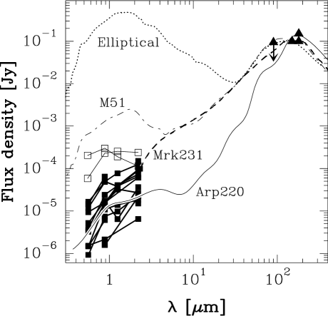
Figure 12: Flux densities of sources with $I$–$K>3.0$ (filled squares) together with the flux densities of the two ISO detections (at 90$\mu$m only an upper limit) in a field within the VCN region. The spectra of the brightest sources with arbitrary $I$–$K$ within 50$\arcsec$ of the FIR source positions are shown as open squares. The spectral energy distributions of two luminous infrared galaxies, Arp 220 (solid line) and Mrk 231 (dashed line), normalized to the 150$\mu$m observations, are drawn for $z\sim$1.0 (Ivison et al. ivison98 (1998)). For comparison, template spectra of an elliptical galaxy (dotted line) and of the spiral galaxy M51 (dash-dotted) are shown for $z=0$ (Silva et al. silva (1998))

7 Conclusions

We have searched for FIR point sources in raster maps observed with the ISOPHOT C100 and C200 detectors at wavelengths between 90$\mu$m and 180$\mu$m. The total area covered is $\sim$1.5 square degrees. Most of the FIR sources detected are presumably IR galaxies which, due to the negative $K$-correction, can be observed at redshifts $z>1$. A comparison of the SEDs of sources detected at 90, 150, and 180$\mu$m with cirrus spectra shows that for most sources an explanation in terms of cirrus knots can be excluded. Based on the number counts of the sources we can conclude:

• We have found 55 FIR sources that, due to the multi-wavelength confirmation, correspond to detections with high confidence level ($\ga$4$\sigma$)

• We have derived a FIR source density of $\sim$60 sources per $\squareforqed\degr$ at 100 mJy level

• The source density is much higher than predicted by no-evolution galaxy models; at 180$\mu$m the excess is close to a factor of five

• The source counts are in agreement with models where the star formation rate and the relative number of ULIGs increases strongly with $z$, e.g. the counts are slightly higher than predicted by model E of Guiderdoni et al. (guiderdoni98 (1998))

• At 150$\mu$m and 180$\mu$m the combined flux of detected sources accounts for $\sim$10% of the CIRB intensity as derived from the COBE FIRAS data; at 90$\mu$m the fraction is over 20%

Appendix A Calibration comparisons

The results presented in this paper are based on the calibration performed with the onboard FCS. This has been estimated to be better than 30% for extended sources brighter than 4 MJy sr^-1 (Klaas et al. klaas98 (1998)). Because of the very low surface brightness and the correspondingly low FCS power, it is interesting to compare the ISO calibration scale with the corresponding DIRBE values.

For the comparison of absolute surface brightnesses we took the DIRBE ZSMA (Zodi-Subtracted Mission Average Maps) data around each ISO field. Zodiacal light was added to the DIRBE values according to the model given by Leinert et al. (leinert98 (1998)) using the $\lambda-\lambda_{\sun}$ and the ecliptic latitude of the ISO observations. We could also have used the Weekly Averaged Sky Map data observed during those weeks when the solar elongation is similar as in the ISO observations. Because of the somewhat lower noise we chose to use the the ZSMA data. Both DIRBE and ISO were colour corrected assuming a $\nu^{2}B_{\nu}$ spectrum and $T_{\rm dust}$=18 K (Arendt et al. arendt (1998); Schlegel et al. schlegel98 (1998)). DIRBE data were interpolated to the wavelength of the ISO observations. The average ISO flux density weighted with the DIRBE beam was compared with the DIRBE value. The surface brightness ratios obtained are shown in Table 6 in column 4. The main uncertainties are due to the large DIRBE beam and the large noise of the DIRBE 140 $\mu$m and 240 $\mu$m observations in these faint surface brightness regions. The given error estimates correspond to the total dispersion in the surface brightness values. These estimates are probably more realistic than those obtained by combining the error estimates calculated for the mean surface brightness values.

Table 6: Comparison of the DIRBE and ISO flux density scales for surface brightnesses. The columns are: (1) the field name, (2) wavelength of ISO observations, (3) mean surface brightness of the ISO map, (4) the ratio of the DIRBE and ISO absolute surface brightnesses. For column 4 the numbers given in parentheses give the dispersions in the DIRBE surface brightness values interpolated to the wavelength of the ISO observations (see text). Note that for EBL22 we have chosen to correct the calibration according to existing absolute photometry measurements

Field	$\lambda$	$<S>$	$S_{\rm DIRBE}/S_{\rm ISO}$
	($\mu$m)	(MJy sr-1)
(1)	(2)	(3)	(4)
EBL26	180	6.0	1.44(0.30)
	150	7.9	1.40(0.29)
	90	15.8	0.79(0.05)
NGPS	180	3.1	1.29(0.17)
	150	3.7	1.24(0.15)
	90	5.7	0.65(0.06)
NGPN	180	1.8	1.67(0.07)
	1801	2.4	1.28(0.03)
	150	2.5	1.43(0.07)
	90	5.5	0.57(0.02)
NGPN & NGPS	180	2.2	1.44(0.23)
	150	3.3	1.31(0.18)
	90	5.6	0.62(0.06)
EBL22	180	2.3	2.25(0.09) [1.21(0.05)]
			1.73(0.07)
	150	2.0	2.00(0.07) [1.24(0.05)]
			1.69(0.06)
	90	0.8	0.80(0.02)
			0.85
ZW II	180	12.6	1.28(0.03)
	120	9.6	1.59(0.04)

¹ the larger 180$\mu$m map
[ ] using default responsivities
italic entries: corrected according to absolute photometry measurements

At 90$\mu$m the DIRBE values are $\sim$30% lower than the ISO values. On the other hand, there is an indication that the ISO C200 values are $\sim$30-40% lower than the DIRBE ones.

At 140$\mu$m and at 240$\mu$m the relative error estimates given for ZSMA surface brightness values exceed in many cases 50%. When the temperature was fixed to 18 K the interpolated values at 150 $\mu$m and 180 $\mu$m are mostly determined by the selected temperature and the 100 $\mu$m DIRBE values which have significantly smaller error estimates. An increase of $T_{\rm dust}$ by 1 K increases $S_{\rm DIRBE}/S_{\rm ISO}$ at 90 $\mu$m by $\sim$1% and decreases it at 150$\mu$m and 180$\mu$m by about 10%. On the other hand, if the exponent in $\nu^{\alpha}$ is decreased from 2.0 to 1.0 the discrepancy between ISO and DIRBE scales would increase at 180$\mu$m by $\sim$20%. If all sources of uncertainty are taken into account our results do not indicate a difference between the ISO and DIRBE flux density scales exceeding $\sim$30%.

In the case of EBL22 there was an unusually large difference, by a factor of $\sim$0.6, between the values obtained with default responsivities and those calibrated with the FCS measurements. The fact that the FCS heating power was clearly below the range for which calibration tables exist may have contributed to the large discrepancy. Comparison with DIRBE supports the higher surface brightness values obtained with the default responsivities (see Table6). Absolute photometry at one position in the field gives values closer to the default calibration. Since the FCS calibration is more reliable in the case of the absolute photometry we have re-scaled the maps to agree with the absolute photometry. For all the other maps the differences between the FCS and the default responsivities remained below 30%.

Appendix B Details of the point source detection

B.1 Flat fielding

Normally the flat fielding was done by calculating the ratios between each detector pixel and the average of other measurements within a small area around it. Linear fits provided the flat fielding correction factors as function of the surface brightness.

In some cases (e.g. in VCN) it was found advantageous to perform the flat fielding partially together with the source fitting. This was done by adding free parameters to scale independently the measurements made with different detector pixels. This introduces to the fit three additional parameters in the case of C200 maps and eight parameters for the C100 maps. Determining the flat fielding (multiplicative factor only) locally makes it possible to automatically correct for some detector drifts. The method is useful when the detector drifts are slow compared with the time needed to observe the region surrounding a point source.

B.2 The fitting procedure

The point source detection was performed in two steps using the surface brightness values and their errors, one value for each detector pixel in each raster position. In the first step measurements more than 0.7$\sigma_{\rm bg}$ above the local background level were flagged as point source candidates. The background level and its dispersion, $\sigma_{\rm bg}$, were estimated from other measurements within a radius which was typically three times the size of the detector pixel.

In the second step a model of a point source and a background was fitted to each region surrounding the candidate positions. The background was assumed to be constant, since in most cases the gradient of the background was small. The free parameters of the fit were the source flux density, the two coordinates of the source position, and the background surface brightness.

The contribution of a point source to the measured flux density at different map positions was computed using the footprint matrices of PIA. Footprint matrices provide the fraction of the flux detected by each detector pixel. Some 70% of the flux from a point source located at the centre of a pixel will be detected by this one pixel. The detector beams are approximately gaussian in their central part but have more extended wings. The neighboring pixels will therefore receive slightly more flux than predicted by the gaussian approximation, about 7% or less for source distances exceeding one pixel step (46.0$\arcsec$ for C100 and 92$\arcsec$ for C200).

The radius of the region used in the fitting procedure was typically $\sim$2.2$\arcmin$ for maps observed with the detector C100 and $\sim$3.7$\arcmin$ for maps done with C200. These radii are large enough to make the contribution from the point source small at the edge of the fitting region.

B.3 Completeness and false detections in simulations

The completeness of the point source detection and the probability of false detections were studied with simulated maps with raster step equal to the detector size i.e. without any redundancy. We simulated the dependence of faint sources detection on the background noise level. The criterion given above was used for selecting the candidate pixels with point source contribution, the probability limit, $P>$99%, was used to discard uncertain detections. Different values of the ratio

$$\rho=\frac{S_{\nu}}{\sigma_{\rm bg}}$$ (3)

between source flux density, $S_{\nu}$, given in Jy and the background rms noise, $\sigma_{\rm bg}$, given in units of Jy were also considered. The detection rate is about 90% for $\rho=7.8$ while for values close to $\rho=$5.2 the detection rate drops below 50%. The number of false detections as the function of the probability limit $P$ was also studied. The number of false detections is, as expected, linear with respect to $P$. However, the number of false sources was found to exceed the expected number of 1-$P$ false detections per map pixel (see Fig. 13a). This was taken into account when determining the parameters of source detection. One would obviously like to have criteria where the number of false detections is equal to the unknown number of undetected real sources.

The flux densities of false detections were found to lie between $S_{\nu}\approx 3.3\sigma_{\rm bg}$ and below $S_{\nu}\approx 7.0\sigma_{\rm bg}$. The lower limit is set partly by the initial selection of candidate pixels that are 0.7$\sigma_{\rm bg}$ above the background noise. The spatial distribution of the false detections is shown in Fig. 13b. They are concentrated close to the edges and the corners of the pixels. The source density varies roughly as $r^{2}$ where $r$ is the distance from the pixel centre. This does not, however, help in eliminating false detections since the spatial distribution is similar for very faint true sources. The bias is present only close to the detection limit.

Figure 13: a The number of false detections per map pixel in simulated measurements as a function of the expected number 1-$P$. The confidence level $P$ is used to discard uncertain detections. At high confidence levels the actual number of false detections exceeds the expected number (dashed line). b Positions of false detections inside a map pixel for non-overlapping rasters. Similar distribution exists for very weak sources

B.4 Influence of imperfect flat fielding and de-glitching

The simulations described above, that were used in determining suitable detection limits, do not take into account some effects that may affect the source counts. For example, imperfect flat fielding or de-glitching will lead to higher surface brightness values in some detector pixels and may increase the probability of classifying some random variations as point sources. The problem is potentially more serious for the C100 detector where the deviation of one detector pixel has less influence on the overall noise of the surface brightness estimated for the region. In those cases where the local flat fielding coefficients were estimated together with the source parameters the quality of the flat fielding is less important. In order to estimate its effect in other cases we simulated C100 measurements consisting first of normally distributed noise and then scaled upwards the values of one detector pixel. The number of false detections did not, however, depend strongly on the imperfections of the flat fielding and was in fact smaller for the tested range where one detector pixel deviated less than 2$\sigma$. If more than one pixel deviates from the mean the effect is further reduced. We conclude that imperfect flat fielding will not cause significant errors in the source counts.

Appendix C Methods in the examination of SRD data

The main procedures used in the source extraction were based on AAP (Astrophysical Applications Data) data products reduced with PIA. The corresponding SRD (Signal per Ramp Data) files were used for visual inspection of the data. Glitches are visible at the SRD level as a sudden high signal value followed by gradually decreasing tail or, in the case of several glitches close in time, as unusually large noise. The number of ramps per raster position varies in our data from 6 to over 40. In the case of the C100 detector, which is more affected by the glitches, the number of ramps was always sufficient to see the characteristic features of the glitches.

The SRD data close to the potential sources were inspected visually in order to check whether the detections were possibly due to glitches and not to real point sources. The raster position and the detector pixel closest to the fitted source position was determined and with the selected raster position in the centre the SRD data for five consecutive raster position and for all detector pixels were plotted (see Fig. 3). Both the variations in the signal level between raster positions and between the different detector pixels were examined by eye and the measurement closest to the source position was checked for signs of glitches. A quality flag between 0 and 4 was given for the source and these are shown in Table 5.1 as flag “q”. The intended scale is:

• 0: the median signal is clearly affected by glitches and/or the noise is clearly too high for reliable determination of the median signal

• 1: there are clear glitches that may have affected the median signal and/or large noise makes the determination of the median uncertain

• 2: no clear signs of a source, no significant glitches

• 3: a possible source

• 4: a clear detection

The difference in the signal levels between different raster positions and between different detector pixels were also used in the scrutinization. Therefore, even if the signals were seriously affected by glitches the source could be classified in e.g. class 3 provided that the true signal level could be estimated to be high enough.

The classification is, of course, subjective. It is also strongly biased towards sources that happen to lie in the centre of some detector pixel and are therefore visible only in one measurement. Furthermore, if the source is situated between two raster lines the previously described SRD vs. time plots do not show all data relevant for the classification.

The main benefit from the eyeball inspection is that we can recognize potentially false detections (classes 0 and 1) that are due to detector glitches. There are, however, only a couple of such possibly false detections in our source sample. This shows that most false detections were avoided in our source detection procedure.

The source detections were tested also by applying to the SRD data methods reminiscent of the procedures used in the ELAIS project (Surace et al. surace99 (1999)).

For each source we determined the raster position and the detector pixel, $p_{\rm 0}$ closest to the potential source. Using the signal values $s_{\rm i}^{\rm p}$ from all detector pixels $p$ from five consecutive raster positions ($i$=-2…2) centered on the selected position we calculated the following values:

1. $s_{\rm 0}^{\rm p_{\rm 0}}/s_{\rm 0}^{\rm p},p\neq p_{\rm 0}$ subtracted by the median of the corresponding values at the five raster positions

2. same as (1.) but instead of the median we use a prediction from 2nd degree fit to the five raster positions

3. $s_{\rm 0}$ subtracted by the median of $s_{\rm i}^{\rm p_{\rm 0}}$, $i$=-2…2

4. same as previous but using prediction from a 2nd degree fit instead of the median

5. $s_{\rm 0}^{\rm p_{\rm 0}}$ divided by the median of other pixels in the current raster position subtracted by the median of the corresponding values in all five raster positions

6. same as previous but using a 2nd degree fit instead of the median of five raster positions

In the case of C100 we calculated therefore altogether 20 values and in the case of C200 10 values. The number of values above 1.5$\sigma$ level was counted and is shown in Table 5.1 as flag “$c$”. It must be emphasized that the method is applied only to the SRD data closest to the previously determined source positions and it is therefore most sensitive to sources that were close to the centre of some detector pixel. Thus a low value of “$c$” does not disqualify a source detection obtained with our detection procedure.

References

- (1) Abraham R.G., Ellis R.S., Fabian A.C. et al., 1999, MNRAS 303, 641
- (2) Arendt R.G., Odegard N., Weiland J.L., et al., 1998, ApJ 508, 74
- (3) Barger A.J., Cowie L.L., Sanders D.B., et al., 1998, Nat 394, 248
- (4) Barger A.J., Cowie L.L., Sanders D.B., 1999, ApJ, 518, L5
- (5) Blain A. W., Smail I., Ivison R.J., Kneib J.-P., 1999a, MNRAS 302, 632
- (6) Blain A. W., Kneib J.-P., Ivison R.J., Smail I., 1999b, ApJ 512, L87
- (7) Cowie L.L., Hu E.M., 1998, AJ 115, 1319
- (8) Cowie L.L., Songaila A., Hu E.M., 1996, AJ 112, 839
- (9) Cowie L.L., Hu E.M., Songaila A., Egami E., 1997, ApJ 481, 9
- (10) Devriendt J.E.G., Guiderdoni B., Sadat R., 2000, A&A, in press
- (11) Dunlop J.S., Hughes D.H., Rawlings S., et al., 1994, Nat 370, 347
- (12) Eales S., Lilly S., Gear W. et al., 1999, ApJ 515, 518
- (13) Efstathiou A., Oliver S., Rowan-Robinson M. et al., 2000, MNRAS, submitted
- (14) Fixsen D.J., Weiland J.L., Brodd S. et al., 1997, ApJ 490, 482
- (15) Fixsen D.J., Dwek E., Mather J.C. et al., 1998, ApJ 508, 123
- (16) Franceschini A., Andreani P., Danese L., 1998, MNRAS 296, 709
- (17) Gautier C., III, Boulanger F., Perault M., Puget J.L., 1992, AJ 103, 1313
- (18) Guiderdoni B., Bouchet F.R., Puget J.-L. et al., 1997, Nat 390, 257
- (19) Guiderdoni B., Hivon E., Bouchet F.R., Maffei B., 1998, MNRAS 295, 877
- (20) Hauser M.G., Arendt R.G., Kelsall T. et al., 1998, ApJ 508, 25
- (21) Heckman T.M., Robert C., Leitherer C., et al., 1998, ApJ 503, 646
- (22) Herbstmeier U., Abraham P., Lemke D., et al., 1998, A&A 332, 739
- (23) Holland W.S., Robson E.I., Gear W.K. et al., 1999, MNRAS 303, 659
- (24) Hu E.M., Cowie L.L., McMahon R.G., 1998, ApJ 502, L99
- (25) Hughes D.H., Dunlop J.S., 1999, In: Highly Redshifted Radio Lines, Carilli C., et al. (eds.), PASP Conference Series Vol. 156
- (26) Hughes D.H., Dunlop J.S., Rawlings S., 1997, MNRAS 289, 766
- (27) Hughes D.H., Serjeant S., Dunlop J., et al., 1998, Nat 394, 241
- (28) Ivison R.J., Smail I., Le Borgne J.-F., et al., 1998, MNRAS 298, 583
- (29) Juvela M., Mattila K., Lemke D., 2000, to appear in the Proceedings of the Meeting ISO Beyond Point Sources, ESA-SP
- (30) Kalluri S., Arce G.R., 1998, IEEE Transactions on Signal Processing Vol. 46, 2, 322
- (31) Kawara K., Sato Y., Matsuhara H., et al., 1998, A&A 336, L9
- (32) Kelsall T., Weiland J.L., Franz B.A. et al., 1998, ApJ 508, 44
- (33) Kessler M.F., Steinz J.A., Anderegg M.E. et al., 1996, A&A 315, L27
- (34) Klaas U., Laureijs R.J., Radovich M., Schulz B., 1998, ‘ISOPHOT Calibration Accuracies’, http://www.iso.vilspa.esa.es/manuals/PHT/accuracies/ pht_accuracies20/
- (35) Lagache G., Abergel A., Boulanger F., Désert F.X., Puget J.-L., 1999, A&A 344, 322
- (36) Leinert C.H., Bowyer S., Haikala L. K., et al., 1998, A&AS 127, 1
- (37) Lemke D., Klaas U., Abolins J., et al., 1996, A&A 315, L64
- (38) Lilly S.J., Eales S.A., Gear W.K.P et al., 1999, ApJ 518, 641
- (39) Linden-Vørnle M.J.D., Nørgaard-Nielsen H.U., Jørgensen H.E. et al., 2000, A&A
- (40) Lisenfeld U., Isaak K.G., Hills R., 2000, MNRAS, in press, astro-ph/9907035
- (41) Low F.J., Cutri R.M., 1994, Infrared Phys. Technol. Vol. 35, No 2/3, 291
- (42) Madau P., Ferguson H.C., Dickinson M.E., et al., 1996, MNRAS 283, 1388
- (43) Oliver S., Serjeant S., Efstathiou A., et al., 2000, in “ISO Surveys of a Dusty Universe”, Lemke D., Stickel M., Wilke K. (eds.), Springer
- (44) Omont A., McMahon R.G., Cox P., et al., 1996, A&A 315, 1
- (45) Puget J.-L., Abergel A., Bernard J.-P., et al., 1996, A&A 308, L5
- (46) Puget J.-L., Lagache G., Clements D.L., et al., 1999, A&A 345, 29
- (47) Schlegel D.J., Finkbeiner D.P., Davis M., 1998, ApJ 500, 525
- (48) Silva L., Granato G.L., Bressan A., Danese L., 1998, ApJ 509, 103
- (49) Smail I., Ivison R.J., Blain A.W., 1997, ApJL 490, L5
- (50) Smail I., Ivison R.J., Blain A.W., Kneib J.-P., 1999, In: “After the Dark Ages: When Galaxies were Young”, Holt S., Smith E. (eds), AIP Press, 312
- (51) Steidel C.C, Giavalisco M., Pettini M., et al., 1996, ApJ 462, L17
- (52) Steidel C.C., Adelberger K.L., Giavalisco M. et al., 1999, ApJ 519, 1
- (53) Stiavelli M., Treu T., Carollo C.M., et al., 1999, A&A 343, L25
- (54) Surace C., Héraudeuau P., Lemke D., et al., 1999, in the proceedings of “The Universe as seen by ISO”, Paris, ESA SP-427, 1059
- (55) van der Werf P.P., 1999, In: The most distant radio galaxies, Röttgering H.J.A., Best P.N., Lehnert M.D. (eds.), Kluwer