The Robustness of Inflation to Changes in Super-Planck-Scale Physics

Abstract

We calculate the spectrum of density fluctuations in models of inflation based on a weakly self-coupled scalar matter field minimally coupled to gravity, and specifically investigate the dependence of the predictions on modifications of the physics on length scales smaller than the Planck length. These modifications are encoded in terms of modified dispersion relations. Whereas for some classes of dispersion relations the predictions are unchanged compared to the usual ones which are based on a linear dispersion relation, for other classes important differences are obtained, involving tilted spectra, spectra with exponential factors and with oscillations. This is the case when the dispersion relation becomes complex. We conclude that the predictions of inflationary cosmology in these models are not robust against changes in the super-Planck-scale physics.

]

I Introduction

Most current models of inflation [1] are based on weakly self-coupled scalar matter fields minimally coupled to gravity. In most of these models, the period of inflation lasts for a number of e-foldings much larger than the number needed to solve the problems of standard cosmology [2]. In these cases, the physical length of perturbations of cosmological interest today (those which today correspond to the observed CMB anisotropies and to the large-scale structure) was much smaller than the Planck length at the beginning of inflation. Hence, the approximations which go into the calculation of the spectrum of cosmological perturbations [3] break down. It is then of interest to investigate whether the predictions are sensitive to the unknown super-Planck-scale physics, or whether the resulting spectrum of perturbations is determined only by infrared physics.

An analogous problem arises for black hole evaporation. The original computations of the thermal spectrum from black holes [4] appear to involve mode matching at super-Planck scales. However, in the case of black holes it can be shown [5, 6, 7, 8] that the predictions are in fact insensitive to modifications of the physics at the ultraviolet end.

Our goal is to explore whether and in which cases the spectrum of fluctuations resulting from inflationary cosmology depends on the unknown ultraviolet physics. We will adapt the method of [5, 8] and consider theories obtained by replacing the linear dispersion relation for the linearized fluctuation equations by classes of nonlinear dispersion relations. We find that for the class of dispersion relations introduced by Unruh [5] one recovers a scale-invariant spectrum of fluctuations in the case of exponential inflation. In contrast, for the class of dispersion relations modelled after the one introduced in [8], the resulting spectrum may be tilted and may include exponential and oscillatory factors if the dispersion relation becomes complex. Such spectra are inconsistent with observations. We thus conclude that the predictions for observables in weakly coupled scalar field models of inflation depend sensitively on hidden assumptions about super-Planck-scale physics.

II Framework

We will consider the evolution of linear cosmological fluctuations in a spatially flat homogeneous and isotropic Universe. As is well known (see e.g. [9] for a comprehensive review), the evolution equation of scalar and tensor fluctuations in conformal time $\eta$ reduces to harmonic oscillator equations with time dependent masses. In the following, we will therefore simply consider the evolution of a scalar field $\Phi(\eta,\bf{x})$ living on space-time. Introducing $\mu(n,\eta)$ via the Fourier transform $\Phi(\eta,{\bf x})\equiv[1/(2\pi)^{3/2}]\int{\rm d}{\bf n}(\mu/a)e^{i{\bf n}\cdot{\bf x}}$ [where $a(\eta)$ is the scale factor], the evolution equation of the mode with a comoving wavenumber $n$ becomes

$$\mu^{\prime\prime}+\biggl{[}n^{2}-\frac{a^{\prime\prime}}{a}\biggr{]}\mu\,=\,0\,.$$ (1)

The corresponding power spectrum $P_{\Phi}(n)$ is given by

$$n^{3}P_{\rm\Phi}\,=\,n^{3}\biggl{|}\frac{\mu}{a}\biggr{|}^{2}\,.$$ (2)

In order to study the dependence of the predictions for $P_{\Phi}$ on super-Planck-scale physics, we will modify the linear dispersion relation $\omega_{\rm p}^{2}=k^{2}=(n/a)^{2}$ (where $\omega_{\rm p}$ is the physical frequency) for wavenumbers greater than a critical wavenumber $k_{\rm C}$ by replacing the $n^{2}$ term in (1) with

$$n_{\rm eff}^{2}\,=\,a^{2}(\eta)F^{2}(k)\,=\,a^{2}(\eta)F^{2}[n/a(\eta)]\,,$$ (3)

where $F(k)$ differs significantly from $k$ only for $k>k_{\rm C}$. We see that, in terms of comoving wavenumbers, we obtain a time dependent dispersion relation.

The two classes of dispersion relations we specifically analyze are the one proposed by Unruh [5] and a generalization of the one studied by Corley and Jacobson [8]. The first class is given by

$$F(k)\,\equiv\,k_{\rm C}\tanh^{1/p}\biggl{[}\biggl{(}\frac{k}{k_{\rm C}}\biggr{)}^{p}\biggl{]},$$ (4)

where $p$ is an arbitrary coefficient. For large values of the wave number, this becomes a constant $k_{\rm C}$ whereas for small values this is a linear law as expected. The second class of dispersion relations is given by

$$F^{2}(k)\,=\,k^{2}+k^{2}b_{m}\biggl{(}\frac{k}{k_{\rm C}}\biggr{)}^{2m},$$ (5)

where $m$ is an integer and the coefficients $b_{m}$ are at this stage arbitrary. Note that for negative $b_{m}$ the dispersion relation becomes complex for $k\gg k_{\rm C}$. The dispersion relations are shown in Fig. 1.

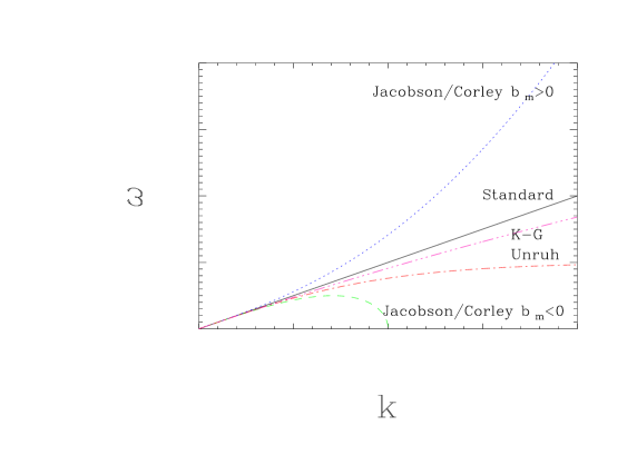
FIG. 1.: Sketch of the different dispersion relations.

In order to compute the power spectrum $P_{\Phi}(n)$ of (2) we need to know both the initial conditions for the mode $\mu(n,\eta)$ and the subsequent evolution. We first discuss the initial conditions. We want the state at the initial time $\eta_{\rm i}$ to correspond as closely as possible to our usual physical intuition of a vacuum state. We here study two prescriptions for this. The first is to canonically quantize the field $\mu(n,\eta)$ and to demand that the initial state minimizes the energy [10]. The second is to set the state up in the local Minkowski vacuum [11]. In the case of a linear dispersion relation, both prescriptions give the same result. However, for a nonlinear dispersion relation, we obtain different results (which emphasizes the general point that the predictions of inflationary cosmology depend on the initial state chosen [12]).

Demanding that the initial state minimize the energy yields [13]

$$\mu(\eta=\eta_{\rm i})\,=\,\frac{1}{\sqrt{2\omega(\eta_{\rm i})}},\quad\mu^{\prime}(\eta=\eta_{\rm i})\,=\,\pm i\sqrt{\frac{\omega(\eta_{\rm i})}{2}}\,,$$ (6)

where $\omega$ is the comoving frequency, whereas prescribing the local Minkowski vacuum state gives

$$\mu(\eta_{\rm i})\,=\,\frac{1}{\sqrt{2n}},\quad\mu^{\prime}(\eta_{\rm i})\,=\,\pm i\sqrt{\frac{n}{2}}\,.$$ (7)

As is apparent from (1), in the case of a linear dispersion relation $\omega=n$ and the two prescriptions for the initial state coincide. It should be clear that the choice (6) is certainly the most physical one. The second choice, as mentioned above, illustrates the fact that the final result does depend on the initial conditions.

III Calculation of Spectra

We now compute the power spectrum $P_{\Phi}(n)$ for values of $n$ with wavenumbers larger than $k_{\rm C}$ at the initial time $\eta_{\rm i}$. On such scales, the time interval can be divided into three regions. The first is $\eta_{\rm i}<\eta<\eta_{1}(n)$, during which the physical wavenumber exceeds $k_{\rm C}$. During this time interval, the mode evolution is non-standard. The second interval lasts from the time $\eta_{1}(n)$ to the time $\eta_{2}(n)$ when the wavelength equals the Hubble radius $l_{\rm H}$. During this time, the solutions of the mode equation (1) are oscillatory since the $n^{2}$ term in the parentheses in (1) dominates over the $a^{\prime\prime}/a$ term. In the third period [$\eta>\eta_{2}(n)$], the modes are effectively frozen: the non-decaying solution of the mode equation is $\mu(\eta)\sim a(\eta)$.

The values of $\eta_{1}$ and $\eta_{2}$ depend on the background evolution. For a power-law inflation model with $a(\eta)=l_{0}|\eta|^{1+\beta}$, where $\beta$ is a number with $\beta\leq-2$ and $l_{0}$ has the dimension of a length, the values of $\eta_{1}$ and $\eta_{2}$ are given by

$$|\eta_{1}(n)|\, = \,\biggl{(}\frac{n}{2\pi}\frac{l_{\rm C}}{l_{0}}\biggr{)}^{1/(1+\beta)}|b_{m}|^{1/[2m(1+\beta)]}\,,$$ (8)

$$|\eta_{2}(n)| = \frac{2\pi}{n}|1+\beta|\,,$$ (9)

where $l_{\rm C}$ is the wavelength corresponding to $k_{\rm C}$. By combining the above formula for $a(\eta)$ with (8), it follows that

$$a[\eta_{2}(n)]^{-2}\,\sim\,n^{2+2\beta}\,.$$ (10)

Assuming that the non-decaying modes mix with coefficients of order unity at the times $\eta_{1}$ and $\eta_{2}$, then based on the above observations about the time dependence of $\mu(n,\eta)$ in the various time intervals, we obtain the following ‘master formula’ for the power spectrum at late times:

$$n^{3}P_{\Phi}(n)\,\sim\,{{n^{3}}\over{2\omega(\eta_{\rm i})}}\biggl{|}{{\mu[n,\eta_{1}(n)]}\over{\mu(n,\eta_{\rm i})}}\biggr{|}^{2}a[\eta_{2}(n)]^{-2}\,.$$ (11)

This result is true if the initial state minimizes the energy density. If the initial state is taken to be the local Minkowski vacuum, then $\omega(\eta_{\rm i})$ on the r.h.s. of (11) needs to be replaced by $n$.

In the case of the linear dispersion relation, $\mu(n,\eta)$ also oscillates during the first time interval $\eta_{\rm i}<\eta<\eta_{1}(n)$. Since in this case $\omega(\eta_{\rm i})\sim n$, we immediately obtain

$$n^{3}P_{\Phi}(n)\,\sim\,n^{4+2\beta}\,,$$ (12)

the ‘standard’ prediction of inflationary cosmology.

In the case of Unruh’s dispersion relation, the mode equation can be solved exactly during the first time interval in the case of exponential inflation ($\beta=-2$):

$$\mu(n,\eta)\,=\,A_{1}|\eta|^{x_{1}}+A_{2}|\eta|^{x_{2}}\,,$$ (13)

where $A_{1}$ and $A_{2}$ are two constant determined by the initial conditions and where the exponents $x_{1}$ and $x_{2}$ are given by

$$x_{1,2}\,\equiv\,\frac{1}{2}\pm\frac{1}{2}\sqrt{9-16\pi^{2}\frac{l_{0}^{2}}{l_{\rm C}^{2}}}\,.$$ (14)

Note that both modes are decaying ($|\mu|\sim\eta^{1/2}$ and $|\eta|\rightarrow 0$). Since $\eta_{1}$ depends on $n$ as given in (8), we have

$${{\mu[n,\eta_{1}(n)]}\over{\mu(n,\eta_{\rm i})}}\,\sim\,n^{-1/2}\,.$$ (15)

Since for the minimum energy density initial state $\mu(n,\eta_{\rm i})$ is independent of $n$ in the wavelength interval under consideration, we obtain

$$n^{3}P_{\Phi}(n)\,\sim\,n^{0}\,,$$ (16)

i.e. the same scale-invariant spectrum as in the case of the linear dispersion relation.

TABLE I.: Spectra for different dispersion relations and different initial conditions. The function $\bar{B}(n)$ is a complicated oscillatory functions which can be found in Ref. [13].

Dispersion Relation	Initial Conditions	Spectrum $n^{3}P_{\rm\Phi}$
Unchanged  ($\omega=k$)	Minimizing energy=Minkowski	$n^{2\beta+4}$
Unruh  ($\beta=-2$)	Minimizing energy	$n^{0}$
Unruh  ($\beta=-2$)	Minkowski	$n^{-1}\cos^{2}\biggl{(}\frac{2\pi}{\epsilon}+\frac{2\pi}{\epsilon}\ln\biggl{|}\frac{2\pi}{n\eta_{\rm i}}\biggr{|}\biggr{)}$
Jacobson/Corley  ($b_{\rm m}<0$)	Minimizing energy	$n^{2\beta+4}e^{An^{m+1}}\cos^{2}\biggl{[}2\pi|1+\beta|-\biggl{(}\frac{\epsilon}{2\pi}\biggr{)}^{\frac{1}{1+\beta}}n^{\frac{2+\beta}{1+\beta}}-\frac{\pi}{4}\biggr{]}$
Jacobson/Corley  ($b_{\rm m}<0$)	Minkowski	$n^{2\beta+4+m}e^{An^{m+1}}\cos^{2}\biggl{[}2\pi|1+\beta|-\biggl{(}\frac{\epsilon}{2\pi}\biggr{)}^{\frac{1}{1+\beta}}n^{\frac{2+\beta}{1+\beta}}-\frac{\pi}{4}\biggr{]}$
Jacobson/Corley  ($b_{\rm m}>0$)	Minimizing energy	$n^{2\beta+4}$
Jacobson/Corley  ($b_{\rm m}>0$)	Minkowski	$n^{2\beta+4+m}|\bar{B}(n)|^{2}$

In the case of the Corley/Jacobson dispersion relation the result is quite different. Let us consider the case $b_{m}<0$ (complex dispersion relation). Then, in the wavelength regime $\lambda(\eta_{\rm i})\ll l_{\rm C}$ of interest, the mode equation in the first time interval can be solved exactly in terms of modified Bessel functions

$$\mu(n,\eta)\,\sim\,|\eta|^{1/2}I_{1/(2b)}(z)\,\sim\,|\eta|^{1/2}[z(\eta)]^{-1/2}e^{z(\eta)}\,,$$ (17)

where the argument of the Bessel function is $z(\eta)\equiv\gamma|\eta|^{b}$ with

$$b\,\equiv\,1-m(1+\beta),\quad\gamma\,\equiv\,{{\sqrt{|b_{m}|}}\over{(2\pi)^{m}b}}\biggl{(}{{l_{\rm C}}\over{l_{0}}}\biggr{)}^{m}n^{m+1}\,.$$ (18)

Note, in particular, the exponential factor in (17) which depends on $n$. This factor does not cancel with any other $n$-dependent term in (11) and is thus the root of the exponential dependence of the final power spectrum on $n$. Combining (11), (6), (10) and (17) we obtain

$$n^{3}P_{\Phi}(n)\, \sim \,n^{3}n^{-1-m}n^{m}e^{2z[\eta_{1}(n)]}n^{2+2\beta}$$ (19)

$$\sim n^{4+2\beta}e^{2z[\eta_{1}(n)]}\,,$$ (20)

where the second factor on the r.h.s. of the first line comes from $\omega(\eta_{\rm i})$, the third and fourth factors stem from the ratio of $\mu$, and the final factor from the $a(\eta_{2})$ term in (11). The careful matching between growing and decaying modes also reveals [13] the presence of an oscillating factor $\cos^{2}(n\eta_{2}-n\eta_{1}-\pi/4)$ in the final power spectrum. However, it should also be noticed that the initial conditions are fixed in a region where the mode function does not oscillate.

In the case of the Corley-Jacobson dispersion relation with $b_{m}>0$, the modified Bessel functions in the mode equation during the first time interval must be replaced by regular Bessel functions. Hence, the exponential factors in the power spectrum disappear and the final result is unchanged, i.e. we recover a scale invariant spectrum.

IV Discussion and Conclusions

We have studied the robustness of the predictions for the spectrum of cosmological perturbations of weakly coupled inflationary models. The method used was to replace the usual linear dispersion relation by special classes of nonlinear ones, where the nonlinearity is confined to physical wavelengths $\lambda$ smaller than some critical length $l_{\rm C}$. We found that for the class of dispersion relations first introduced by Unruh [5], the predictions are unchanged. This is connected with the fact that the initial vacuum state evolves adiabatically up to the time $\eta_{1}$ when $\lambda=l_{\rm C}$ . However, in the case of the dispersion relation modelled after the one used by Corley and Jacobson [8] in the situation where it becomes complex, the resulting spectrum can have oscillations, non-standard tilts and exponential factors which render the resulting theory in conflict with observations. The specific predictions depend on the sign of $b_{m}$, on the value of $m$, and on the initial state chosen. The results are summarized in Table 1.

We thus conclude that the predictions in weakly coupled scalar field-driven inflationary models are not robust to changes in the unknown fundamental physics on sub-Planck lengths. This opens up another potentially very interesting link between fundamental physics and observations. Note, however, that in strongly coupled scalar field models of inflation such as the model discussed in [14], the spectrum of fluctuations is robust to changes in the underlying sub-Planck-length physics.

Acknowledgements

We are grateful to Lev Kofman, Dominik Schwarz, Carsten Van de Bruck and in particular Bill Unruh for stimulating discussions and useful comments. We acknowledge support from the BROWN-CNRS University Accord which made possible the visit of J. M. to Brown during which most of the work on this project was done, and we are grateful to Herb Fried for his efforts to secure this Accord. One of us (R. B.) wishes to thank Bill Unruh for hospitality at the University of British Columbia during the time when this work was completed. J. M. thanks the High Energy Group of Brown University for warm hospitality. The research was supported in part by the U.S. Department of Energy under Contract DE-FG02-91ER40688, TASK A.

REFERENCES

- [1] A. Guth, Phys. Rev. D23, 347 (1981).
-
[2]
A. Linde, D. Linde and A. Mezhlumian, Phys. Rev.
D49, 1783 (1994);
A. Linde, ‘Lectures on Inflationary Cosmology’, Stanford preprint SU-ITP-94-36, hep-th/9410082 (1994). -
[3]
G. Chibisov and V. Mukhanov, ‘Galaxy Formation and
Phonons,’ Lebedev Physical Institute Preprint No. 162 (1980);
V. Mukhanov and G. Chibisov, JETP Lett. 33, 532 (1981);
V. Mukhanov and G. Chibisov, Sov. Phys. JETP 56, 258 (1982);
G. Chibisov and V. Mukhanov, Mon. Not. R. Astron. Soc. 200, 535 (1982);
V. Lukash, Pis’ma Zh. Eksp. Teor. Fiz. 31, 631 (1980);
A. Starobinsky, Phys. Lett. 117B, 175 (1982);
S. Hawking, Phys. Lett. 115B, 295 (1982);
A. Guth and S. Y. Pi, Phys. Rev. Lett. 49, 1110 (1982);
J. Bardeen, P. Steinhardt, and M. Turner, Phys. Rev. D28, 679 (1983). - [4] S. Hawking, Comm. Math. Phys. 43, 199 (1975).
- [5] W. Unruh, Phys. Rev. D51, 2827 (1995).
- [6] R. Brout, S. Massar, R. Parentani and P. Spindel, Phys. Rev. D52, 4559 (1995).
- [7] N. Hambli and C. Burgess, Phys. Rev. D53, 5717 (1996)
-
[8]
S. Corley and T. Jacobson, Phys. Rev. D54, 1568 (1996);
S. Corley, Phys. Rev. D57, 6280 (1998). - [9] V. Mukhanov, H. Feldman, and R. Brandenberger, Phys. Rep. 215, 203 (1992).
- [10] M. Brown and C. Dutton, Phys. Rev. D18, 4422 (1978).
- [11] R. Brandenberger, Nucl. Phys. B245, 328 (1984).
- [12] J. Martin, A. Riazuelo and M. Sakellariadou, Phys. Rev. D61, 083518 (2000). astro-ph/9904167.
- [13] J. Martin and R. Brandenberger, ‘The Trans-Planckian Problem of Inflationary Cosmology’, Brown preprint BROWN-HET-1214.
- [14] R. Brandenberger and A. Zhitnitsky, Phys. Rev. D55, 4640 (1997).