AN OVERVIEW OF THE SPOrt EXPERIMENT

Abstract

The Sky Polarization Observatory is an experiment selected by ESA for the Early Opportunity Phase onboard the International Space Station. SPOrt is the first payload specifically designed for polarization measurements, it will provide near full sky maps of the sky polarized emission at four microwave frequencies between 22 and 90 GHz. Current design of SPOrt will be presented, together with an overview of the scientific goals of the experiment.

1 Introduction

The study of the polarized emission at microwave frequencies is fundamental to understand the physical processes in our Galaxy. Moreover, the galactic emission represents a foreground noise in Cosmic Background Radiation (CBR) anisotropy experiments. Finally, the polarized component of the CBR contains more information about our universe than CBR anisotropies, in particular concerning the nature of the primordial fluctuations and the re-ionization era.

The Sky Polarization Observatory (SPOrt) is a space experiment devoted to measure the sky polarized emission in the microwave domain (20-90 GHz) with 7^∘ beamwidth. It is the first scientific payload specifically designed to make a clean measurements of the Q and U Stokes parameters. SPOrt radiometers, in fact, are optimized for this purpose by adopting:

- simple optics (corrugated feed horns) to avoid additional spurious polarization from off-axis reflections;

- low cross-polarization antenna system;

- Q and U correlated outputs.

Main features of the SPOrt experiment are summarized in Table 1, for a detailed description of SPOrt technical issues see [1].

During its 18 months lifetime, SPOrt will provide the first high frequency, high sensitivity ($5\div 10\mu$K) polarization maps of the sky, mapping the synchrotron emission at lower frequencies (20-30 GHz) and attempting the detection of the polarized component of the CBR.

SPOrt is totally sponsored by the Italian Space Agency (ASI) and it has been selected by the European Space Agency (ESA) to fly on the International Space Station (ISS) in 2003.

Table 1: SPOrt characteristics

Frequencies	Bandwidth	Angular	Instantaneous	Lifetime
(GHz)		resolution	sensitivity
22, 32, 60, 90	10%	$7^{\circ}$	$1mKs^{\frac{1}{2}}$	1.5 yrs

2 The polarized emission of the sky

Sky polarized emission comes both from non-cosmological (galactic and extragalactic) and from cosmological (CBR) sources. In the following sections, the main characteristics of both the galactic (“foreground”) and the CBR polarized emission are summarized, under the assumption that extragalactic polarized emission (coming from point sources) should be considered negligible at SPOrt resolution.

2.1 The galactic polarized emission

The galatic emission arises from three different physical processes:

- synchrotron, which is produced by relativistic electrons moving in the galactic magnetic field;

- bremsstrahlung (free-free), which comes from interactions between free electrons and ions in a highly ionized medium;

- dust emission, which has thermal origin.

So far data on polarized emission above 5 GHz are lacking. Maps at 408, 465, 610, 820, 1411 MHz are provided by [2] and, more recently, low latitude galactic surveys have been carried out by [3] (at 2.4 GHz) and [4], [5] (at 1.4 GHz).

This means that expected polarized emission at SPOrt frequencies can be evaluated only by extrapolating low frequency data.

In general, predictions on both polarized and unpolarized sky emission are different from author to author due to different assumptions on the normalization of the various foregrounds (see e.g. [6] and [7]). There is, instead, a general agreement on foregrounds frequency behaviour. Synchrotron ($T_{S}$) and free-free ($T_{F}$) brightness temperature are usually approximated by a power law, while dust brightness temperature emission ($T_{D}$) is modelled with a mixture of two greybodies (cfr. [8]):

$$\begin{array}[]{rlrl}T_{S}&\propto\nu^{S}&S&=-(2.6\div 3.2)\\ T_{F}&\propto\nu^{F}&F&\simeq-2.15\\ T_{D}&\propto\nu^{D-2}\left[B_{\nu}(20.4\mbox{K})+6.7\cdot B_{\nu}(4.77\mbox{K})\right]&D&\simeq 2\end{array}$$

While synchrotron and dust emission are intrinsicly polarized, bremsstrahlung can be polarized only via anisotropic Thomson scattering within optically thick HII regions; expected polarization degrees on SPOrt angular scales are $<30\%$ for synchrotron and $\leq 10\%$ for free-free and dust.

Figure 1 shows the expected polarized foregrounds. The following normalizations have been used: $T_{S}(30$ GHz$)=18\mu$K (dotted line), $T_{F}(30$ GHz$)=2\mu$K (dashed line), and $T_{D}(200$ GHz$)=1\mu$K (dash dotted line).

Figure 1: Expected sky polarized emission in the microwave domain: CBR (dashed strip) for two different values of normalization (5-0.2% of CBR temperature anisotropies i.e. maximum and minimum $P(7^{\circ})$ values in Figure 2, respectively), synchrotron (dotted line), free-free (dashed line) and dust (dashed-dotted line); symbols show the upper limits on CBR polarization from previous experiments (see Table 2); horizontal ticks show the expected pixel (min and max) and full sky sensitivities, respectively, for SPOrt at its four frequencies (see Table 3).

For a detailed discussion on foreground emissions see [7]. However some remarks should be done:

- Maps at low frequencies show that the synchrotron power index varies with position. A frequency dependence of the spectral index is also expected: the break frequency of the synchrotron spectrum depends on the break on the energy distribution of cosmic rays and on the (spatially varying) value of the galactic magnetic field.

- Emission from spinning dust grains has been introduced by [9] to explain correlations between $30\div 40$ GHz galactic emission and DIRBE-FIRAS data ([10], [11], [12]). It would dominate over free-free and synchrotron in the $10-60$ GHz frequency range and would be intrinsicly polarized for $\nu<40$ GHz ([13]).

2.2 The CBR Polarization

The CBR is the most valuable witness of the early universe and CBR anisotropy investigations are a powerful tool to determine fundamental cosmological parameters such as the total density of the universe $\Omega_{\circ}$, the Hubble constant $H_{\circ}$, the baryon density $\Omega_{b}$ and the cosmological constant $\Lambda$ ([14]).

Same informations could be provided by the CBR polarization which, in addition, represents the only way able to test the inflationary paradigm, to determine the nature (scalar or tensorial) of the primordial perturbations and to constraint the ionization history of the universe (see e.g. [15] and references therein).

The polarization of the CBR is generated by Thomson scattering of the anisotropic CBR radiation field in the cosmic medium, thus its intensity is only a fraction of the CBR temperature anisotropy; depending on the epoch of the scattering, its spectrum shows the maximum power at different angular scales corresponding to the particle horizon dimension at that epoch. For the Standard Cold Dark Matter (SCDM) model the peak occurs at $\leq 1^{\circ}$ angular scales, while for recombination models the maximum emission occurs at $5^{\circ}-7^{\circ}$ angular scales.

Expected polarized emission at $7^{\circ}$ angular scales for a SCDM and various recombination models are reported in Figure 2. The minimum and the maximum values of $P(7^{\circ})$ represent the boundary of the dashed strip in Figure 1; in this way foreground and CBR polarized emission can be compared easily.

Figure 2: Expected CBR polarized emission (in terms of polarized brightness temperature, $P=\sqrt{Q^{2}+U^{2}}$) smoothed to 7^∘ calculated for $\Omega_{b}=0.05$, $H_{0}=50$ vs reionization redshift $z_{ri}$. Values are calculated for three different ionization fractions ($x_{e}$). Solid horizontal line represents SPOrt full sky sensitivity at $2\sigma$ level.

None of the past and current CBR polarization experiments have led to a positive detection so far. Table 2 and Figure 1 report available upper limits only, in fact, the most stringent being $18\mu$K on a $1^{\circ}.4$ scale near the North Celestial Pole ([21]).

Table 2: Upper limits on CBR polarization from previous experiments.

Frequency	Angular	Sky	Upper limit	Ref	Fig. 1
(GHz)	Resolution	coverage
4.0	15∘	scattered	300 mK	[17]	X
100-600	1∘.5 - 40∘	GC	3-0.3 mK	[18]
9.3	15∘	$\delta$ = +40∘	1.8 mK	[19]	+
33	15∘	$\delta\in$ (-37∘, +63∘)	180 $\mu$K	[16]	*
5.0	18” - 160”	$\delta$ = +80∘	4.2 mK - 120 $\mu$K	[20]	diamond
26-36	1∘.2	NCP	30 $\mu$K	[21]	triangle
26-36	1∘.4	NCP	18 $\mu$K	[22]	square

3 The SPOrt Correlation Receiver

Correlation techniques are widely adopted in high sensitivity measurements because of their capability to reduce gain fluctuations.

Residual gain fluctuations are usually recovered, both for polarization and for total power experiments, using destriping techniques (see [23], [24]), which require a “good” radiometer stability within a single scan period.

Being not a free flyer, SPOrt has a scanning period (i.e. the orbital period of the ISS $\sim$ 90 mins) larger than other microwave space experiments (for instance COBE and MAP have $\sim 1\div 2$ min. scanning periods). In spite of this, the applicability of an efficient destriping technique is based by the high stability of the SPOrt correlation radiometers.

By correlating the linear ($E_{x}$ and $E_{y}$) and circular ($E_{r}$ and $E_{l}$) components of the incoming radiation the following quantities can be obtained:

$$U=2E_{x}E_{y}\cos{\epsilon} Q=2E_{r}E_{l}\cos{\delta}=2E_{r}E_{l}\cos{2\theta}$$

$$V=2E_{x}E_{y}\sin{\epsilon} U=2E_{r}E_{l}\sin{\delta}=2E_{r}E_{l}\sin{2\theta}$$ (1)

where $\epsilon$ and $\delta$ are the phase difference of the two linear and circular components respectively, V is the Stokes parameter describing the circular polarization, and $\theta$ is the polarization angle.

Thus, having to deal with linear components, a simultaneous correlated Q and U output cannot be obtained. After a first measurement that gives U, in fact, the radiometer has to be rotated by $45^{\circ}$ in order to have Q. The correlation of circular components, instead, provides a simultaneous measurement of the Stokes parameters Q and U.

SPOrt adopts this second technique: a block diagram of a SPOrt radiometer is shown in Figure 3.

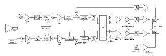
Figure 3: Block diagram of one SPOrt polarimeter

The antenna system provides left handed and right handed circular components to low noise radiometric chains, which feed the correlation unit (i.e. Hybrid Phase Discriminator (HPD), zero bias diodes and differential amplifiers). The HPD outputs:

$$\left\{\begin{array}[]{l}\frac{1}{\sqrt{2}}\cdot\left(E_{r}-jE_{l}\right)\\ \frac{1}{\sqrt{2}}\cdot\left(E_{l}+jE_{r}\right)\\ \frac{1}{\sqrt{2}}\cdot\left(E_{r}-E_{l}\right)\\ \frac{1}{\sqrt{2}}\cdot\left(E_{r}+E_{l}\right)\\ \end{array}\right.$$ (2)

are then square law detected:

$$V_{1} = k\left[\left(E_{r}^{2}+E_{l}^{2}\right)+2E_{r}E_{l}\cos{\delta}\right]$$

$$V_{2} = k\left[\left(E_{r}^{2}+E_{l}^{2}\right)-2E_{r}E_{l}\cos{\delta}\right]$$

$$V_{3} = k\left[\left(E_{r}^{2}+E_{l}^{2}\right)+2E_{r}E_{l}\sin{\delta}\right]$$

$$V_{4} = k\left[\left(E_{r}^{2}+E_{l}^{2}\right)-2E_{r}E_{l}\sin{\delta}\right]$$ (3)

Finally, after differential amplification and integration, Q and U are obtained:

$$V_{1}-V_{2} = kE_{r}E_{l}\cos{\delta}\propto Q$$

$$V_{3}-V_{4} = kE_{r}E_{l}\sin{\delta}\propto U$$ (4)

4 Expected performances

A simulation of the SPOrt experiment sensitivity has been carried out ([25]) using the radiometer equation:

$$\sigma_{f}=\frac{\sigma_{1s}}{\sqrt{\tau}}$$ (5)

where $\tau$ is the total integration time and $\sigma_{1s}$ is the instantaneous radiometer sensitivity. It showed how the scanning method of SPOrt makes the sensitivity depending on the sky direction. Figure 4 shows integration time across the sky after the expected 18 months experiment lifetime.

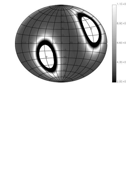
Figure 4: SPOrt sky coverage after 18 months, the banner shows the integration time in seconds after 1.5 yrs.

SPOrt final expected sensitivities are reported in Table 3 and in Figure 1, they are calculated assuming a 50% observing efficiency, i.e. rejecting half of the data; “full sky” sensitivity is calculated by averaging the signal over the whole sky.

Table 3: Expected sensitivities for SPOrt, 50% observing efficiency has been assumed

Max Pixel Sensitivity	Min Pixel Sensitivity	Full Sky Sensitivity	Sky Coverage
($\mu$K)	($\mu$K)	($\mu$K)
4.0	8.0	0.26	82 %

As it can be seen from Figure 1, SPOrt frequencies have been chosen to satisfy the two main experiment’s aims:

- SPOrt lowest frequency channels (20-32 GHz) lie in a foreground dominated spectral window;

- The highest frequency channels (60-90 GHz) could be exploited to detect CBR polarized emission in a spectral window were foreground emission has its minimum.

5 Conclusions

The SPOrt experiment is expected to measure the sky polarized emission in an unexplored frequency window with expected sensitivity $\sim 50$ times better than the best existing upper limit on CBR polarization. SPOrt should reach these goals thanks to its wide frequency coverage that includes the “cosmological window” ($\sim 60-100$ GHz) of minimum expected foreground emission. Such a sensitivity, together with the extended sky ($>80$%) and frequency coverage should allow to put new and quite severe constraints on the CBR polarization at degrees angular scales. Finally, it would be pointed out that the very simple SPOrt layout configuration has been mainly imposed by the need to match the ISS environment, but it represents anyway a new approach to very sensitive polarization measurements.

Acknowledgements Authors acknowledge ESA for the encouragement and partial financial support of the SPOrt project, as well as ASI for the full approval and funding of the SPOrt Program. A special thank is for all the SPOrt collaboration. Figure 2 has been produced by using the CMBFast ([26]) software and Healpix package ([27]).

References

- [1] S. Cortiglioni, S. Cecchini, E. Carretti, M. Orsini, R. Fabbri, G. Boella, G. Sironi, M. Gervasi, M. Zannoni, J. Monari, A. Orfei, R. Tascone, U. Pisani, K.W. Ng, L. Nicastro, L. Popa, I.A. Strukov, M.V. Sazhin in proceedings of the International Conference on 3K Cosmology EC-TMR Conference, AIP Conference Proceedings, 476, pp.194-203, 1998 - astro-ph/9901362.
- [2] W.N. Brouw, T.A.Th. Spoelstra, Astronomy and Astrophysics Supplement, 26, pp. 129-146, 1976.
- [3] A.R. Duncan, R.F. Haynes, K.L. Jones, R.T. Stewart, MNRAS, 291, pp. 279-295, 1997.
- [4] B. Uyaniker, E. Fuerst, W. Reich, , P. Reich, R. Wielebinski, Astronomy and Astrophysics Supplement, 132, pp. 401-411, 1998.
- [5] B. Uyaniker, E. Fuerst, W. Reich, , P. Reich, R. Wielebinski, Astronomy and Astrophysics Supplement, 138, pp. 31-45, 1999.
- [6] B. Keating, P. Timbie, A. Polnarev, J. Steinberger, The Astrophysical Journal, 495, pp. 580, 1998.
- [7] R. Fabbri, S. Cortiglioni, S. Cecchini, M. Orsini, E. Carretti, G. Boella, G. Sironi, J. Monari, A. Orfei, R. Tascone, U. Pisani, K.W. Ng, L. Nicastro, L. Popa, I.A. Strukov, M.V. Sazhin in proceedings of the International Conference on 3K Cosmology EC-TMR Conference, AIP Conference Proceedings, 476, pp.194-203, 1998 – astro-ph/9901363.
- [8] A. Kogut, A.J. Banday, C.L. Bennett, K.M. Gorski, G. Hinshaw, W.T. Reach, The Astrophysical Journal, 460, pp. 1-9, 1996.
- [9] B.T. Draine, A. Lazarian, The Astrophysical Journal, 494, pp. L19-L22, 1998.
- [10] A. Kogut, astro-ph/9902307, 1999.
- [11] A. De Oliveira-Costa, M. Tegmark, C.M. Gutierrez, A.W. Jones, R.D. Davies, A.N. Lasenby, R. Rebolo, R.A. Watson, astro-ph/9904296, 1999.
- [12] A. De Oliveira-Costa, M. Tegmark, L.A. Page, S.P. Boughn, The Astrophysical Journal, 509, pp. L9-L12, 1998.
- [13] B.T. Draine, A. Lazarian, astro-ph/9902356, 1999.
- [14] M. White, D. Scott, J. Silk, Annual Review of Astronomy and Astrophysics, 32, pp. 319-370, 1994.
- [15] M. Kamionkowski, A. Kosowsky, A. Stebbins, Phys. Rev. D, 55, 7368, 1997.
- [16] P.M. Lubin, G.F. Smoot, The Astrophysical Journal, 245, pp. 1-17, 1981.
- [17] A.A. Penzias, R.W. Wilson, The Astrophysical Journal, 142, pp. 419-421, 1965.
- [18] N. Caderni, R. Fabbri, F. Melchiorri, V. Natale, Phys. Rev. D, 17, pp. 1901-1907, 1978.
- [19] G.P. Nanos, The Astrophysical Journal, 232, pp. 341-347, 1979.
- [20] R.B. Partridge, J. Nowakowski, H.M. Martin, Nature, 331, pp. 146-147, 1988.
- [21] E.J. Wollack, N.C. Jarosik, C.B. Netterfield, L. Page, D. Wilkinson, The Astrophysical Journal, 419, pp. L49-L52, 1993.
- [22] C.B. Netterfield, N. Jarosik, L. Page, D. Wilkinson, E.J. Wollack, The Astrophysical Journal, 445, pp. L69-L72, 1995.
- [23] J. Delabrouille, Astronomy and Astrophysics Supplement, 127, pp. 555-567, 1998.
- [24] E.L. Wright, astro-ph/9612006.
- [25] M. Orsini, L. Nicastro, E. Carretti, S. Cortiglioni I.Te.S.R.E. C.N.R. Internal Report, #233/99, 1999.
- [26] See CMBFAST Website: http://www.sns.ias.edu/matiasz/CMBFAST/cmbfast.html
- [27] See the Healpix home page: http://www.tac.dk/healpix