On cooling flows and the Sunyaev-Zel’dovich effect

Abstract

We study the effect of cooling flows in galaxy clusters on the Sunyaev-Zel’dovich (SZ) distortion and the possible cosmological implications. The SZ effect, along with X-ray observations of clusters, is used to determine the Hubble constant, $H_{\circ}$. Blank sky surveys of SZ effect are being planned to constrain the geometry of the universe through cluster counts. It is also known that a significant fraction of clusters has cooling flows in them, which changes the pressure profile of intracluster gas. Since the SZ decrement depends essentially on the pressure profile, it is important to study possible changes in the determination of cosmological parameters in the presence of a cooling flow. We build several representative models of cooling flows and compare the results with the corresponding case of gas in hydrostatic equilibrium. We find that cooling flows can lead to an overestimation of the Hubble constant. Specifically, we find that for realistic models of cooling flow with mass deposition (varying $\dot{m}$ with radius), there is of the order $\sim 10\%$ deviation in the estimated value of the Hubble constant (from that for gas without a cooling flow) even after excluding $\sim 80\%$ of the cooling flow region from the analysis. We also discuss the implications of using cluster counts from SZ observations to constrain other cosmological parameters, in the presence of clusters with cooling flows.

1. Introduction

Galaxy clusters are extensively observed in optical, X-ray and radio bands. In the radio band, a cluster can be observed in the the Rayleigh-Jeans side of the cosmic microwave background spectrum, as a dip in the brightness temperature, due to Sunyaev-Zel’dovich effect (SZ) (Sunyaev & Zel’dovich 1972; for a comprehensive review, see Birkinshaw 1999). The SZ distortion appears as a decrement for wavelengths $\geq 1.44$ mm (frequencies $\leq 218$ GHz) and as an increment for wavelengths $\leq 1.44$ mm. SZ effect has the advantage that the SZ intensity, unlike that of the X-ray, does not suffer from the $(1+z)^{-4}$ cosmological dimming. As discussed by numerous authors (Birkinshaw & Hughes 1994; Silverberg et.al. 1997), one can combine the X-ray and radio observations for clusters to determine cosmological parameters. This has been done in the recent years to determine the Hubble constant $H_{\circ}$ (Birkinshaw 1999). The SZ signal is, however, weak and difficult to detect. Recent high signal to noise detection have been made over a wide range in wavelengths using single dish observations: at radio wavelengths (Herbig et al, 1995, Hughes & Birkinshaw 1998), millimeter wavelengths (Holzapfel et al. 1997, Pointecouteau et al. 1999) and submillimeter wavelengths (Komatsu et al. 1999). Interferometric observations have also been carried out to image the SZ effect (Jones et al. 1993, Saunders et al. 1999, Reese et al. 1999, Grego et al. 2000). Other than estimating $H_{\circ}$ combining SZ and X-ray data, SZ effect alone can also be used to determine the cosmological mass density $\Omega_{\circ}$ of the universe (Bartlett & Silk 1994, Oukbir & Blanchard 1992, 1997, Blanchard & Bartlett 1998). However, these procedures generally assume the cluster gas is spherical, unclumped and isothermal. Almost all clusters, however, show departures from these simplistic assumptions with some to a large extent.

Departures from these simple assumptions can lead to systematic errors in the determination of the different cosmological parameters (Inagaki et al 1995), especially, it was seen that non-isothermality of the cluster can lead to a substantial error in values of the cosmological parameters. Temperature structure in a cluster can be the result of the shape of the gravitational potential (Navarro et al 1997, Makino et al 1998), or it can arise due to the fact that the initial falling gas in the cluster potential is less shock heated than the later falling gas (Evrard 1990). In fact hydrodynamical simulations of isolated clusters also show a definite temperature structure and can introduce error in the value of $H_{\circ}$ when compared to the traditional isothermal $\beta$-models (Yoshikawa 1998). Roettiger et al (1997) have shown that cluster mergers can result in deviations from both sphericity and isothermality. Observationally, the main handicap arises from the fact that the thermal structure of clusters are hard to measure, and the temperatures generally taken in analyses are the X-ray emission weighted temperature, usually measured over a few core radii. So, in general an isothermal description of the cluster is taken (or sometimes a phenomenological temperature model based on the Coma cluster: for example see Eq 73 of Birkinshaw 1999).

In this paper, we study another important phenomenon that can substantially change the temperature structure, viz. a cooling flow. Cooling flows in clusters of galaxies (for an introduction, see Fabian et al 1984) is a well established fact by now, and it is seen that around $60-90\%$ of clusters exhibit cooling flows in their core with $\approx 40\%$ of them having cooling flows of more than $100M_{\odot}~{}yr^{-1}$ (Markevitch et al 1998, Peres et al 1998, Allen et al 1999). In the largest systems, the mass deposition rate can be as high as $1000M_{\odot}~{}yr^{-1}$ (Allen 2000). The idealised picture of a cooling flow is as following: Initially when the cluster forms, the infalling gas is heated from gravitational collapse. With time this gas cools slowly and a quasi hydrostatic state emerges. However in the central region, where energy is lost due to radiation faster than elsewhere, an inward ‘cooling flow’ initially arises due to the pressure gradient (Fabian 1994). This can modify the SZ decrement and act as a systematic source of error in the determination of the cosmological parameters.

Schlickeiser (1991) has shown that free-free emission from cold gas in the cooling flow can actually lead to an apparent decrease of the SZ effect at the centre. Since the central cooling flow region is generally very small, the isothermal $\beta$-model of cluster gas can still be used for the majority of cluster region even for cooling flow cluster, with the extra precaution of excluding the central X-ray spike from the X-ray fit, and a corresponding change made in the fitting of the SZ decrement. This is only possible for nearby clusters, however with well resolved cluster cores.

Naively, the change in the central SZ decrement $y(0)$ can be seen as follows : For a non cooling flow cluster, the central decrement is given by the line of sight integral of the electron pressure through the cluster centre along the full extent of the cluster. If the cluster has a maximum radius $r_{cl}$, then the central SZ decrement at RJ wavelengths can be written as $y(0)=-4{{\sigma_{T}}\over{m_{e}c^{2}}}\int_{0}^{r_{cl}}p_{e}dl$. For a cluster with a cooling flow, let us suppose that the electron pressure $p_{e}$, drastically falls below a certain radius $r_{s}$, which is typically well inside the core of the cluster. The resulting central decrement is then $y(0)\approx-4{{\sigma_{T}}\over{m_{e}c^{2}}}\int_{r_{s}}^{r_{cl}}p_{e}dl$. Depending on the distance of $r_{s}$ from the cluster centre [$r_{s}\approx(0.1$ to  $0.3)r_{core}$],there wiil be a change in the value of $y(0)$ by $\approx 5\%-25\%$. However, this simplistic view may not be true. This estimate assumes that the pressure profile remains a $\beta$ profile outside the radius $r_{s}$. The pressure profile, however, need not follow the $\beta$ profile once cooling flow starts and it can deviate from it substantially even for radii much larger than $r_{s}$. As a matter of fact, there can actually be an increase in the pressure for a large region inside the cooling flow, before a sudden drop inside $r_{s}$. Since the usual proecedure for estimating the Hubble constant depends on fitting $\beta$ profiles to the SZ and X-ray profiles, to estimate $r_{core}$, this change in the pressure profile due to cooling flow can distort the estimation of $r_{core}$ and hence, the value of $H_{\circ}$ in a non-trivial way. We study this effect in detail in later sections.

In this paper, we have investigated the problem of cooling flow induced change in the temperature and density profile, its effect on the SZ effect, and its subsequent effect on the determination of cosmological parameters. In §2 we briefly review the physics of Sunyaev Zel’dovich effect; §3 is devoted to the physics of cooling flows and discussing the cooling flow solutions; in §4 we look at the effect of cooling flow solutions on SZ effect, both on the determination of $H_{\circ}$ and $\Omega_{\circ}$; we conclude in §5 with a brief comment on how this work differs from other work and the relevance of this paper. For the SZ effect, our notation and approach mainly follows that described in Barbosa et al(1996).

2. Determining Hubble constant with Sunyaev-Zel’dovich effect

2.1. The Sunyaev-Zel’dovich Effect

The integral of the electron pressure along any line-of-sight through the cluster determines the magnitude of the distortion of the apparent brightness temperature of the cosmic microwave background (CMB) due to SZ effect. This is quantified in terms of the Compton $y$-parameter:

$$y=\int{dl}{{k_{B}T_{e}}\over{m_{e}c^{2}}}n_{e}\sigma_{T},$$ (1)

where $k_{B}$ is the Boltzman constant, $T_{e}$ is the gas temperature, $m_{e}$ is the electron rest mass, $n_{e}$ is the electron number density, $c$ is the velocity of light and $\sigma_{T}$ is the Thomson scattering cross-section. This occurs through the inverse-Compton scattering, by the hot intracluster gas, of the CMB photons propagating through the cluster medium, and the energy transfer in this interaction between hot electrons and CMB photons resulting in a distortion to the CMB spectrum. The SZ surface brightness at a position $\theta$ of the cluster with respect to the mean CMB intensity is given by

$${\delta\textit{i}_{\nu}(\theta)=\textit{y}(\theta)\textit{j}_{\nu}(x),}$$ (2)

x is a dimensionless frequency parameter

$$x={{h\nu}\over{kT_{o}}},$$ (3)

where $h$ is the Planck constant, $\nu$ is the observing frquency and $T_{0}$ is the CMB temperature at the present epoch: $T_{0}\sim 2.73$K. The function ${j}_{\nu}(x)$ describes the spectral shape of the effect

$$\textit{j}_{\nu}(x)={{2(kT_{\circ})^{3}}\over{(hc)^{2}}}{{x^{4}e^{x}}\over{\left(e^{x}-1\right)}^{2}}\left[{{x}\over{\tanh\left(x/2\right)}}-4\right].$$ (4)

Since the total photon number is conserved in the inverse Compton scattering process, upscattering of the photons, the spectral dependance gets an unique shape, through a decrement in the brightness temperature at lower frequencies while an increase is observed at higher frequencies.

The Sunyaev-Zel’dovich effect provides a unique observing approach to traditional methods — which use X-ray temperature and X-ray luminosity. The X-ray studies have a major disadvantage because of ‘cosmological dimming’, the surface brightness of distant X-ray sources falls off as $(1+z)^{-4}$, and for this reason, obtaining samples of clusters at cosmological distances is challenging. The SZ effect has the distinct advantage of being independent of the distance to the cluster. The SZ flux density from a cluster will diminish with distance to the cluster as the square of the angular-size distance; in contrast to X-ray flux densities from clusters which diminish as the square of the luminosity distance to the cluster. If the observations resolve clusters, particularly at lower redshifts, the observed sky SZ temperature distribution will be sensitive to the thermal electron temperature structure within the clusters; once again this may be contrasted with X-ray emission images of cluster gas distributions which are mainly sensitive to the gas density distribution.

2.2. Determination of Hubble constant

The method for the determination of Hubble constant using Sunyaev-Zel’dovich effect uses two observable quantities : 1) $\Delta T/T$ of the CMB due to SZ effect; 2) the X-ray surface brightness $S_{X}$ of the cluster. These can be written as

$${{\Delta T_{SZ}}\over{T}}(r)=-2\int_{l_{min}}^{l_{max}}{{k_{B}T_{e}}\over{m_{e}c^{2}}}\sigma_{T}n_{e}dl,$$ (5)

$$S_{X}(r)={{1}\over{4\pi{(1+z)}^{4}}}\int_{l_{min}}^{l_{max}}{{dL_{X}}\over{dV}}dl,$$ (6)

where $r$ is the distance to the line of sight from the cluster centre, $l_{max}$ and $l_{min}$ give the extension of the cluster along the line of sight, ${{dL_{X}}\over{dV}}$ is the X-ray emissivity and $dl$ the line element along the line of sight. The X-ray emissivity in the frequency band $\nu=\nu_{1}$ to $\nu_{2}$ can be written as

$${{dL_{X}}\over{dV}}={n_{e}}^{2}\alpha(T_{e};\nu_{1},\nu_{2},z),$$ (7)

where

$$\alpha(T_{e};\nu_{1},\nu_{2},z)={{2}\over{1+X}}{\left[{{2\pi}\over{3m_{e}c^{2}}}\right]}^{1/2}{{16{e}^{6}}\over{3\hbar m_{e}c^{2}}}A(T_{e};\nu_{1},\nu_{2},z),$$ (8)

where

$$A(T_{e};\nu_{1},\nu_{2},z)=\int_{u_{1}(1+z)}^{u_{2}(1+z)}{(k_{B}T_{e})}^{1/2}e^{-u}$$

$$[{Xg_{ff}(T_{e},u,1)+(1-X)g_{ff}(T_{e},u,2)}]du.$$ (9)

In the above equations we have assumed primordial abundance of hydrogen and helium and have set $X=0.76$, $e$ is the electron charge, $\hbar=h/(2\pi)$, $u\equiv 2\pi\hbar\nu/{k_{B}t_{e}}$, and $g_{ff}(T_{e},u,Z)$ is the velocity averaged Gaunt factor for the ion of charge Ze (Kellog 1975). Traditionally, to model the cluster gas distribution one takes the following density and temperature profiles (Cavaliere & Fusco-Femiano 1978)

$$n_{e}(r)=n_{e0}\left[1+{\left({{r}\over{r_{core}}}\right)}^{2}\right]^{-3\beta/2},$$ (10)

$$T_{e}(r)=T_{iso}=constant,$$ (11)

where $n_{e0}$ is the central electron density and $r_{core}$ the core radius of the cluster. The above expressions are used as an empirical fitting model, and the parameter $`\beta^{\prime}$ is regarded as the fitting parameter. The equation holds for $0<r<R_{cluster}$, where $R_{cluster}$ is the maximum ‘effective’ extension of the cluster. Conventionally, $R_{cluster}=\infty$, and then from equations (5),(6),(10),(11), we get

$${{\Delta T_{SZ}}\over{T}}(\theta) = -{{2\sqrt{\pi}\sigma_{T}k_{B}T_{iso}}\over{m_{e}c^{2}}}n_{e0}r_{core}{{\Gamma(3\beta/2-1/2)}\over{\Gamma(3\beta/2)}}$$ (12)

$$\times{\left[1+{({{d_{A}\theta}\over{r_{core}}})}^{2}\right]}^{1/2-3\beta/2},$$

$$S_{X}(\theta) = {{\sqrt{\pi}}\over{4\pi{(1+z)}^{4}}}\alpha{n^{2}_{e0}}r_{core}{{\Gamma(3\beta-1/2)}\over{\Gamma(3\beta)}}$$ (13)

$$\times{\left[1+{({{d_{A}\theta}\over{r_{core}}})}^{2}\right]}^{1/2-3\beta},$$

where $\Gamma(x)$ is the gamma function. Since both the central CMB decrement and the X-ray surface brightness are observed, one can then combine equations (12) and (13) to estimate the core radius as

$$r_{c,est} = {{{\left[{{\Delta T(\theta)}\over{T}}\right]}^{2}_{obs}}\over{{S_{X}(\theta)}_{obs}}}{{\Gamma(3\beta-1/2){\Gamma(3\beta/2)}^{2}}\over{{\Gamma(3\beta/2-1/2)}^{2}\Gamma(3\beta)}}$$

$${{m_{e}^{2}c^{4}\alpha}\over{16{\pi}^{3/2}{(1+z)}^{4}{\sigma_{T}k_{B}T^{2}_{e,fit}}}}{\left[1+{({{\theta}\over{\theta_{X,core}}})}^{2}\right]}^{-1/2}.$$

In the above equation $\theta_{X,core}$ is the angular core radius observed in X-ray, and $T_{e,fit}$ is the X-ray flux averaged temperature (obtained from fitting the observed X-ray spectrum to the theoretical spectrum expected from isothermal case). This X-ray emission weighted temperature is given by

$$T_{iso}\equiv{{\int_{0}^{r_{vir}}T_{e}(r)\alpha{n_{e}}^{2}r^{2}dr}\over{\int_{0}^{r_{vir}}\alpha{n_{e}}^{2}r^{2}dr}}.$$ (15)

The point to be noted is that $r_{vir}$ is the virial radius of the cluster and its choice depends on the observer. If the temperature has a spatial structure then the $T_{iso}$ inferred from such a procedure may give different values depending on how much of the cluster is taken in making the above average. It has been seen (Yoshikawa et al 1998), that this can lead to a substantial change in SZ effect inferred, and thus to the value $H_{\circ}$.

The angular diameter distance $d_{A}$ can be approximated for nearby ($z\ll 1$) clusters as

$$d_{A}={{cz}\over{H_{\circ}}}\left[1+{{2\Lambda-\Omega_{\circ}-6}\over{4}}z+O(z^{2})\right].$$ (16)

Thus finally we have got an estimate of $d_{A}(z)$ as $r_{c,est}/\theta_{X,core}$. Now, if from other observations we know the cosmological parameters $\Omega_{\circ}$ and $\Lambda$, then one can estimate the Hubble constant

As can be seen from the above equations, the value of $H_{\circ}$ depends crucially on the many assumptions of isothermality and $\beta$-model density distribution of the cluster. Cooling flow changes both of these and so it can significantly affect the value of the Hubble constant.

3. Cooling flows in clusters

3.1. Preliminaries

From X-ray spectra of clusters, it is known that the continuum emission is thermal Bremsstrahlung in nature and originates from diffuse intracluster gas with densities $10^{-2}-10^{-4}~{}cm^{-3}$ and temperatures around $10^{7}-10^{8}$ K. The gas is usually believed to be in hydrostatic equilibrium. If, however, the density in the inner region is large enough, so that the cooling time is less than the age of the cluster, then there is a ‘cooling flow’ (Fabian et al 1984 and references therein). Of course there would be a flow only when the dynamical time is also shorter than the cooling time scale ($t_{age}>t_{cool}>t_{dyn}$).

The basic equations of cooling flow are:

$${du\over dr} = -{u\over\rho_{b}}{d\rho_{b}\over dr}-{2u\over r}-{\dot{\rho_{b}}\over\rho_{b}},$$

$$u{{du}\over{dr}}+{{1}\over{\rho_{b}}}{{d(\rho_{b}\theta)}\over{dr}} = -{{GM_{t}(r)}\over{r^{2}}},$$

$$u{{d}\over{dr}}\left({{3\theta}\over{2}}\right)-{{\theta u}\over{\rho_{b}}}{{d\rho_{b}}\over{dr}} = {{\rho\Lambda(\theta)}\over{{(\mu m_{p})}^{2}}},$$ (17)

where $\theta=2k_{B}T/\mu m_{p}$, $\mu$ is the mean molecular weight, and $m_{p}$ is the proton mass. For steady flows with constant mass flux, $\dot{\rho}=0$. This implies $u=\dot{m}/4\pi\rho r^{2}$ for steady flows. (Note that in cooling flows both $u$ and $\dot{m}$ are negative. The subscripts $b$ refers to baryons and $t$ refers to total i.e baryons + dark matter. However, we assume the baryonic contribution to the total mass negligible w.r.t to the dark matter contribution.)

$M(r)$ describes the distribution of the total mass and depends on the details of dark matter density profiles (see below). $\Lambda(\theta)$ is the cooling function defined so that $n_{e}n_{p}\Lambda(\theta)$ is the rate of cooling per unit volume. We use an analytical fit to the optically thin cooling function as given by Sarazin & White (1987),

$$\bigl{(}{\Lambda(\theta)\over 10^{-22}\,{\rm erg}{\rm cm}^{3}{\rm s}^{-1}}\big{)}=4.7\times\exp\bigl{[}-\bigl{(}{T\over 3.5\times 10^{5}{\rm K}}\bigr{)}^{4.5}\bigr{]}$$ (18)

$$+ 0.313\times T^{0.08}\exp\bigl{[}-\bigl{(}{T\over 3.0\times 10^{6}{\rm K}}\bigr{)}^{4.4}\bigr{]}$$

$$+ 6.42\times T^{-0.2}\exp\bigl{[}-\bigl{(}{T\over 2.1\times 10^{7}{\rm K}}\bigr{)}^{4.0}\bigr{]}$$

$$+ 0.000439\times T^{0.35}\,.$$

This fit is accurate to within $4$% accuracy, for a plasma with solar metallicity, within $10^{5}\leq T\leq 10^{8}$ K. For $10^{8}\leq T<10^{9}$ K, it underestimates cooling by a factor of order unity (compared to the exact cooling function , as in, e.g., Schmutzler & Tscharnuter, 1993) , and therefore is a conservative fit to use, as far as the effect of cooling is concerned.

For non-steady flows, we adopt the formalism of White & Sarazin (1987), where the mass deposition rate, $\dot{\rho}$, is characterised by a ‘gas-loss efficiency’ parameter $q$. One writes $\dot{\rho}=q(\rho/t_{cool})$ where $t_{cool}$ is the local isobaric cooling rate ($t_{cool}=5k_{B}T\mu m_{p}/\rho\Lambda$). It has been found that $q\sim 3$ models can reproduce the observed variation of mass flux ($\dot{m}\propto r$) (Sarazin & Graney 1991). Fabian (1994) has noted that these models of White & Sarazin (1987) yield good approximations to the emission weighted mean temperature and density profiles for cooling flow clusters. We also note that Rizza et al (2000) have used the steady flow models of White & Sarazin (1987) to simulate cooling flows.

We first discuss cooling flows with $\dot{m}=$constant. With $q=0$, one can eliminate the density from Eq. 17 to get two differential equations:

$${{du}\over{dr}} = {u\over\left[r^{2}(5\theta-3u^{2})\right]}\left[3GM-10r\theta+{{\dot{m}}\over{2\pi}}{{\Lambda(\theta)}\over{{uM}^{2}}}\right]$$

$${{d\theta}\over{dr}} = {2\over\left[r^{2}(5\theta-3u^{2})\right]}\left[\theta(2u^{2}r-GM)-(u^{2}-\theta){{\dot{m}}\over{4\pi}}{{\Lambda(\theta)}\over{{uM}^{2}}}\right]$$ (19)

These equations have singularities at the sonic radius $r_{s}$ where $5\theta_{s}=3u_{s}$. A necessary condition of singularity is that the numerators of Eq. 19 vanish at the sonic radius. Therefore (Mathews & Bregman 1978)

$$r_{s}=(3/10\theta_{s})\left[GM(r)+{{\dot{m}\Lambda(\theta_{s})}\over{10\pi\theta_{s}M^{2}}}\right]$$ (20)

We have used two different dark matter profiles for the cluster. The first model ( Model A) has been discussed earlier in the literature in the context of cooling flows in cluster (White & Sarazin 1987; Wise & Sarazin 1993) with a density profile,

$$\rho_{d}=\left\{\begin{array}[]{ll}{\rho_{o}\over 1+(r/r_{core})^{2}}+{\rho_{o,g}\over 1+(r/r_{c,g})^{2}}&\mbox{if $r<237$ kpc}\\ {\rho_{o}\over 1+(r/r_{core})^{2}}&\mbox{if $r>237$ kpc}\end{array}\right.$$ (21)

Here $\rho_{o}=1.8\times 10^{-25}$ gm cm^-3 and $r_{core}=250$ kpc describe the profile of the cluster mass, and $\rho_{o,g}=4.1\times 10^{-22}$ gm cm^-3 and $r_{c,g}=1.69$ kpc describe the profile of the galaxy in the centre of the cluster.

Model B does not have the galaxy in the center, and so it is described simply by $\rho=\rho_{0}/[1+(r/r_{core})^{2}]$.

With these assumptions, the solutions for steady cooling flows, $\dot{m}=$ constant) are fully characterized by (1) the inflow rate, $\dot{m}$, and (2) the temperature of the gas $T_{s}$ at the sonic radius $r_{s}$. Obviously, the cooling flow solutions are only valid within the cooling radius $r_{cool}$ where $t_{cool}=t_{age}$. We assume a value of $t_{age}=10$ Gyr for all models. We assume that outside the cooling radius, gas obeys quasi-hydrostatic equilibrium (Sarazin 1986). Although this means matching the cooling flow solutions with nonzero $u$ to $u=0$ solutions outside, in reality the velocity of gas at the cooling radius is very small (for a $\dot{m}=100$ M_⊙ yr^-1 with $\rho\sim 10^{-26}$ gm cm^-3, at $r=250$ kpc implies a velocity of $30$ km s^-1), which is close to the limit of turbulence in the cluster gas (Jaffe 1980), and smaller than the sound velocity ($\sim 1.5\times 10^{3}\,(T/10^{8}\,K)^{1/2}$ km s^-1). The velocity of the flow at the cooling radius is, therefore, for all practical purposes, sufficiently small to be matched to the solution of hydrostatic equilibrium outside. (In this approach, we avoid the time consuming search for the critical value of $\dot{m}$ for which the flow solutions behave isothermally at $r\rightarrow\infty$ (see Sulkanen et al. 1993).)

As in the usual assumptions for the interpretation of SZ effect, we assume that the gas outside the cooling radius is isothermal, with a constant temperature profile. The density, therefore, obeys $\rho\propto[1+(r/r_{core})^{2}]^{-3\beta/2}$, where $\beta=\mu m_{p}\sigma^{2}/k_{B}T_{iso}$, and $T_{iso}$ is the temperature of the gas at and outside the cooling radius.

For models with non-zero $q$ (Model C: has the same mass profiles as Model A), the solutions are characterized by $T_{s}$ and the value of $\dot{m}$ at the cooling radius, $\dot{m}_{cool}$. Since a fraction of mass drops out of the flow in this case, the inflow velocity need not rise fast and so it is possible to find completely subsonic solutions.

3.2. Cooling flow solutions

We numerically solved the flow equations for the parameters listed in Table 1. The density, temperature and pressure profiles for three cases are presented in Figures 1, 2 & 3 . We mark the position of $r_{cool}$ in each case, and we mark $r_{s}$ for the cases of transonic flows (when $\dot{m}=$ constant). Beyond $r_{cool}$ we match a hydrostatic solution, as explained above, for the respective potentials. We also present, for comparison, the behaviour if the solutions outside $r_{cool}$ are assumed to extend inwards (that is, if no cooling flow is assumed). We will postpone the discussion on the effect of these profiles on the SZ decrement to a later section, and only discuss the qualitative aspects of the solutions here.

The solution A1 is similar to that presented by Wise & Sarazin (1993) (their Figure 1; although they chose to characterise the solutions by the temperature at $r_{cool}$ and not $T_{s}$ as we have done here). It is also similar (qualitatively) to the solution for A262 presented by Sulkanen et al. (1989). As the latter authors have noted, the effect of having a galactic potential in the center is to have a flatter temperature profile for $r>r_{s}$, than in the case of no galactic potential. This aspect is clearly seen while comparing our solutions with and without galactic potentials in the center. Our calculations for the case without the central galaxy are admittedly flawed in the very inner regions where the gas density is larger than the dark matter density, which results in an incorrect determination of the graviational potential in the inner region. However, this happens only inside a region $\sim 25$ kpc from the centre, and should not influence our final results by a large extent.

A word of explanation for the pressure profiles is in order here. Naively speaking, it would appear that the pressure profile inside the cooling radius should have lower values than the corresponding case of hydrostatic equilibrium. The fact that it is not always so has been noted in the literature (e.g., Soker & Sarazin 1988, Fig 1 of Sulkanen et al. 1989 ). The reason for the pressure bump just outside of the sonic radius is that the flow in this inner region is not pressure driven, but rather by gravity (see also Soker & Sarazin 1988). This is why the bump in the profile depends on the presence and absence of the galaxy in the centre. And this profile leads to the curious result that the presence of cooling flow can lead to the overestimation of the Hubble constant as discussed in the next section

The model with mass deposition (C1) is shown in Figure 3. The local mass flux is found to be almost proportional to the radius, consistent with various observations (Fabian, Nulsen & Canizares 1984; Thomas et al. 1987), and, therefore, is probably a realistic model for cooling flow clusters. In this case the temperature drops gradually all the way through, since the velocity does not rise too fast. The deposited mass is assumed to impart negligible pressure and the pressure refers only to that of gas taking part in the flow.

4. Determination of Hubble constant

In this section we discuss the SZ and X-ray profiles of clusters with cooling flows. We compare these with profiles from cluster having gas in hydrostatic equilibrium, and comment on the reliability of measuring Hubble constant. The effect of cooling flow and the subsequent increased Bremsstrahlung emmison is seen in the sudden increase in the X-ray flux in the innermost region of the cluster (Figure 5). The signature of the cooling flow is seen in the form of the central spike in the X-ray profile. The X-ray profile is only affected slightly by the drop in temperature and it is the dependence on the gas density that holds . The temperature dependance becomes important only near the sonic point. Outside $r_{cool}$, the X-ray profile is the same as that in the hydrostatic cases.

The SZ distortion is proportional to the line of sight integral of the pressure, and the sudden increase of the gas density inside the cooling radius is moderated by the decrease of the gas temperature. As a result there is a gradual increase in the gas pressure. Near the sonic point the temperature drops drastically by orders of magnitude, and results in sudden decrease in pressure. However, since this change in pressure becomes acute only within $\approx 5\%$ of the core radius, it contributes negligibly to the line-of-sight integral of the gas pressure, and leads to an increase in the SZ distortion inside the cooling radius for all models considered (see Figure 4). Like the X-ray profiles, the SZ profiles outside $r_{cool}$ is the same as that for the corresponding hydrosstatic cases.

The SZ profiles have been calculated in the Rayleigh-Jeans limit ($x\ll 1$) where $j_{\nu}(x)$ of Eqn. 4 goes to $-2$. In general, however, the profiles should be calculated using Eqn 2. Our results below are independent of the observational frequency, since the profiles at different frequencies have similar shapes, with the amplitude of the SZ distortion scaled either up or down.

Once both profiles are known, one can determine the deviation in the value of the Hubble constant using Eqns(14) & (16). The deviation from the idealistic case can be parametrised as

$$f_{H}\equiv{{r_{core,true}}\over{r_{core,est,fit}}}={{H_{0,est}}\over{H_{0,true}}}$$ (22)

The above formula has been used to determine the deviation of the estimated value of $H_{\circ}$ from the actual value, for models listed in Table-1. The effect of cooling flow on the determination of the cosmological parameters are summarised in Table-2.

To begin with, one has to get best fitted values for $r_{core}$ (or $\theta_{c}$) and $\beta$ from different profiles. Since, the estimation of the Hubble constant depends on the determination of these parameters from the profiles, we look at this issue in more detail. We must keep in mind that the best fitted value of $r_{core}$ (or $\theta_{c}$) and $\beta$ depends on whether one decides to fit the X-ray or the SZ profiles, and the choice can lead to significant differences in the estimated value of $H_{\circ}$. One of the reasons for the strong dependance on the nature of the profile can be the non-isothermality of the cluster gas. Recent observations indicate that intracluster gas has a temperature structure, see Markevitch et al 1998. This is because the y-parameter depends on the integral over $T_{e}$, while emissivity of thermal Bremsstrahlung depends on $\sqrt{T_{e}}$. The dependance of the Gaunt factor on $T_{e}$ isindirect and weak. Yoshikawa et al 1998 have shown that gas temperature drop in the central regions (their Fig. 3), should increase both $r_{core}$ and $\beta$ fitted to $y(\theta)$, and to alesser extent to $S_{X}(\theta)$, as compared to those compared to $n_{e}(r)$. This discrepancy increases at higher redshifts. However, in their case, there is little change in the gas density profile. Clumpiness can also give rise to different fits, resulting in an overestimation of the Hubble constant (Inagaki etal 1995).

There are two other important points that have to be kept in mind while fitting the profiles. First, we must remember that we are trying to fit a cluster having a finite profile with the formulae (Eqns 12 & 13) for isothermal $\beta$ profiles which is derived assuming the cluster to be of infinite extent. This can, by itself, lead to an overestimation of $H_{\circ}$ (Inagaki et al 1995). Thus to have a good fit one must choose a segment of the profile such that, within that segment, the profiles (SZ or X-ray) for a finite cluster do not differ much from those of a hypothetical cluster of infinite extent. We found that SZ and X-ray profiles of clusters start differing from those of infinite size at radii greater than $1.5$ times the core radius. Hence, we have restricted our fitting to radii within $1.5r_{core}$.

Next, one must also be careful to exclude the region close to the sonic point, so that the X-ray spike is excluded from the fit. Also, the central portion in the SZ profile should be avoided as its inclusion can give an apparent central decrement less than its neighbouring points (see Schlickeiser 1991). We have fitted the SZ and X-ray profiles varying the inner cutoff radius and the results for a representative solution for each class of model are tabulated in Tables 3 & 4. Thus, all fittings were done for profiles extending from $r=r_{min}$ to $r=1.5r_{core}$.

As can be seen from Table-2, cooling flows can lead to an overestimation of the Hubble constant. However, we must emphasise, that it may not be possible to a priori estimate the amount of bias introduced in the measurement of the Hubble constant due to cooling flows. There is no simple correlation between the amount of cooling (i.e $\dot{m}$) and the change in the estimated $H_{\circ}$ from the actual value. The total change depends not only on $\dot{m}$, but also on the position of cooling radius, sonic radius, temperature at the sonic point and the isothermal temperature characterising the hydrostatic cases, with which comparisons are made. Specifically, the fitted values of $r_{core}(\theta_{c})$ and $\beta$ for cooling flow models differ from hydrostatic models according to shape of underlying profiles, which is marked by two important features, firstly the central excess of X-ray flux (or excess decrement of SZ flux), and secondly the the deviation from the smooth hydrostatic profile inside $r_{cool}$, the amount of overestimation mainly depends on these factors. For models with a central galaxy potential, there is always an over-estimation of $H_{\circ}$, which is greater than the models without the central galaxy.

For the realistic cases of models C1 and C2, where we have a variable $\dot{m}$ with $r$ inside the cooling radius, the deviation of estimated Hubble constant from its actual value is almost the same. They are also greater than that of models A and B, having similar mass flow rates. This may be due to the fact that the maximum deviation in pressure from the hydrostatic cases is more in non steady cases, than in steady flows. Also non-steady cases are marked by the absence of the sonic radii and the subsequent drop in temperature.

We note that although the different choice of fitting may change the absolute determination of cosmological parameters, the trend i.e deviation from the correct values remains more or less unaffected. It is interesting to note that for B-type model (C1), which include mass deposition in cooling flows, the deviations decrease as one excludes a greater part of the cooling flow region (Table 4& 5). The other models show an increase instead. Here, we remind ourselves that models with mass deposition i.e C-type models are more realistic (Fabian 1994). It is possible that the unsually high value of deviation (Table 4) and the counter-intuitive trend of increasing deviation with decreasing portion of cooling flow region used for fitting (Table 4 & 5), arise because of the unrealistic modelling of cooling flows. If we take the model B1 as a realistic one, then Table 4 & 5 show that to obtain a value of the Hubble constant within an accuracy of $\sim 10\%$, one should have $r_{min}\sim 0.8r_{cool}$. In most cases, $r_{cool}<r_{core}$ (Fabian et al. 1984). However, as $r_{cool}$ cannot be determined without actually detecting a cooling flow in a cluster, we suggest that a significant portion of the profile within $r_{core}$ should be excluded as a precaution. The SZ and the X-ray profiles for the different models are shown in Figures 4 & 5.

5. Discussions and Conclusion

Our work on the effect of temperature structure of clusters and its effect on SZ decrement differs from other previous work of this nature in following way: this work takes into account the change in density profile as well as the temperature profile since both becomes important in the central region of the cluster. Also, previous authors have looked at the issue of non-isothermality of a cluster at radii greater than the core radius of the cluster, whereas we look at temperature change at regions inside the core radius. For them the density profile can still be well approximated by a $\beta$ profile, whereas for cooling flow solutions, density profile is vastly different. Further, they have neglected radiative cooling in their work. We for the first time look at SZ effect in presence of radiative cooling, by first solving the cooling flow equations for reasonable and physical solutions.

In summary, we find that the presence of a cooling flow in a cluster can lead to an overestimation of the Hubble constant determined from the Sunyaev-Zel’dovich decrement. We have used different models of cooling flows, with and without mass deposition, and found the deviation in the estimated value of the Hubble constant in the case of a cooling flow from that of hydrostatic equilibrium. We have used the usual procedure of fitting the SZ and X-ray profile with a $\beta$ profile to get an estimated value of $r_{core}$, and then compared with that for the case of gas in hydrostatic equilibrium in order to estimate the deviation in the Hubble constant. For the more realistic models with mass deposition (varying $\dot{m}$ with radius), we found that the deviation decreases with the exclusion of greater portions of the cooling flow region. Quantitatively, we found that for the deviation to be less than $\sim 10\%$, one should exclude a portion of the profile upto $\sim 0.8r_{cool}$. Since $r_{cool}$ is difficult to estimate without actually detecting a cooling flow, we have suggested that a significant portion of the profile inside $r_{core}$ should be excluded, to be safe.

There can be another important implication of the effect of cooling flows. With the upcoming satellite missions (MAP & Planck), we have come to the point where there are efforts to constrain $\Omega_{0}$ with surveys of blank SZ fields (Bartlett et al 1998; Bartlett 2000), ultimately giving rise to SZ-selected catalog of clusters (Aghanim et al 1997). This method relies on estimating the number of SZ sources brighter than a given threshold flux (Barbosa et al 1996). The point to be noted is that since these surveys are essentially flux limited in nature, the validity of the analysis to determine $\Omega_{0}$ depends crucially on the one-to-one association of flux-limits to corresponding mass limits of clusters. From our analysis above, it seems that it may not be possible to associate a unique cluster mass to a given SZ distortion, given the uncertainty due to the presence of cooling flows. This might lead to contamination in SZ cluster catalogs and the inference of $\Omega_{0}$. Recently, attempts have been made to constrain $\Omega_{\circ}$ from variance measurement of brightness temperature in blank fields (Subrahmanyan et al 1998) and comparing them to simulated fields (Majumdar & Subrahmanyan, 2000), of cumulative SZ distortions from a cosmolgical distribution of clusters. These results may also be systematically affected due to the presence of clusters having cooling flows.

The estimations made in this paper strictly applies to cases where the image of the SZ effect is directly obtained by single dish observations. For interferometric observations, the interferometer samples the fourier transform of the sky brightness rather than the direct image of the sky. The fourier conjugate variables to the right ascension and declination form the $u-v$ plane in the fourier domain. Due to spatial filtering by an interferometer, it is necessary that models be fitted directly to the data in the $u-v$ plane, rather that to the image after deconvolution. We do not forsee drastic change from our inferences in such cases since the result mainly depends on the deviation of the SZ and X-ray profile in case of a cooling flow from those in hydrostatic equilibrium. This, however, should be looked in greater detail in future. We also note that with the growing number of high quality images of the SZ effect with interferometers, which have greater resolution than single dish antennas, the shape parameters of the clusters can be directly determined from the SZ dataset rather than from an X-ray image (Grego et al. 2000).

Finally, we would like to add, though the calculations presented in this paper were done using the dark matter profile (Eqn. 21), which is ”commonly used” for calculating cooling flow solutions, it is inconsistent with the dark matter profile (Navarro et al 1997) found in numerical simulations. (For a comparison of mass and gas distribution in clusters having cooling flows with different dark matter profiles, see Waxman & Miralda-Escude’, 1995). Moreover, we have neglected the self gravity of the gas. Suto et al (1998) have calculated the effect of including the self gravity of the gas in determining the gas density profile. To make strong conclusions about the effect of cooling flows in the determination of the Hubble constant, one should take both the points mentioned above into account.

Table 1 – Parameters for cooling flow solutions

Solution	Mass Model	q	$\dot{m}(r_{cool})$	$T_{s}$	$r_{s}$	$r_{cool}$	$T_{iso}$
			(M⊙ yr-1)	(K)	(kpc)	(kpc)	(K)
A1	Model A	0	100	$6.5\times 10^{6}$	$0.688$	$127.5$	$1.2\times 10^{8}$
A2	Model A	0	200	$6.5\times 10^{6}$	$0.462$	$96.1$	$7.7\times 10^{8}$
A3	Model A	0	300	$6.5\times 10^{6}$	$0.712$	$132.2$	$7.7\times 10^{8}$
B1	Model B	0	100	$4.0\times 10^{6}$	$0.688$	$85.7$	$1.14\times 10^{9}$
B2	Model B	0	200	$6.5\times 10^{6}$	$0.462$	$89.6$	$1.9\times 10^{9}$
B3	Model B	0	300	$6.5\times 10^{6}$	$0.712$	$110.3$	$1.9\times 10^{9}$
C1	Model A	3	200			$111.6$	$1.1\times 10^{8}$
C2	Model A	3	300			$132.2$	$1.1\times 10^{8}$

Table 2 – Effect on central decrement and $H_{\circ}$ for $r_{min}=0.1r_{core}$

Solution Type	${{H_{est}}\over{H_{true}}}$	$\Delta y_{0}$
		(% change)
A1	$1.91$	$35$
A2	$1.18$	$11.5$
A3	$2.6$	$25$
B1	$1.36$	$12.0$
B2	$1.19$	$9.0$
B3	$1.13$	$8.5$
C1	$2.6$	$14.0$
C2	$2.7$	$11.3$

Table 3 – Fitting of SZ profile and deviation of $H_{\circ}$ for $\dot{m}=200m_{\odot}/yr$

Solution Type	$r_{min}=0.2r_{cool}$	$r_{min}=0.5r_{cool}$	$r_{min}=0.8r_{cool}$
	$H/H_{true}$	$H/H_{true}$	$H/H_{true}$
A2	$1.57$	$1.74$	$2.18$
B2	$1.44$	$1.58$	$2.06$
C1	$2.20$	$1.18$	$1.07$

Table 4 – Fitting of X-ray profile and deviation of $H_{\circ}$ for $\dot{m}=200m_{\odot}/yr$

Solution Type	$r_{min}=0.5r_{cool}$	$r_{min}=0.8r_{cool}$	$r_{min}=0.9r_{cool}$	$r_{min}=0.95r_{cool}$
	$H/H_{true}$	$H/H_{true}$	$H/H_{true}$	$H/H_{true}$
A2	–	$4.7$	$2.7$	$1.7$
B2	–	$4.9$	$2.24$	$1.6$
C1	$1.69$	$1.12$	$1.02$	$\approx 1.0$

Figure 1.— Cooling flow solution A2. The upper left panel shows the dark matter density profile (dotted line), the gas density profile for the cooling flow (solid line) and the corresponding case of gas in hydrostatic equilibrium. The lower left panel shows the temperature profiles for the same cases. The position of $r_{s}$ and $r_{cool}$ are shown. The upper right panel shows the pressure profiles and the lower right panel plots the Mach number of the cooling flow gas as a function of the radius.

Figure 2.— Same as figure 1, for cooling flow solution B2.

Figure 3.— Same as figure 1, for cooling flow solution C1.

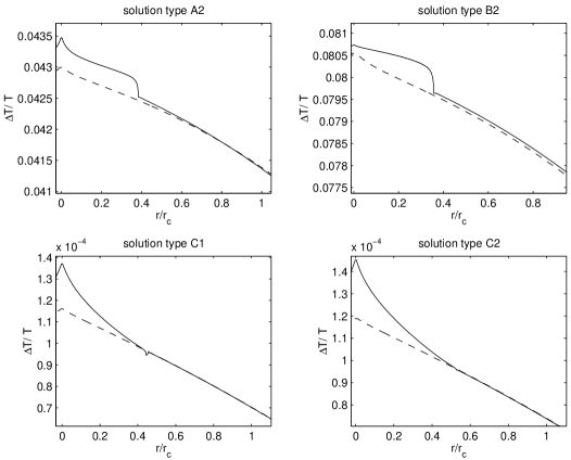
Figure 4.— Unconvolved SZ profiles, for the solution types A2 (upper left), B2 (upper right), C1 (lower left) and C2 (lower right), for cooling flow (solid line) and thecorresponding cases of gas in hydrostatic equilibrium (dashed line). ${{\Delta T_{RJ}}\over{T_{CMB}}}$ is plotted against ${{r}\over{r_{core}}}$. Individual plots have been magnified to highlight the differences between cooling flow and hydrostatic cases.

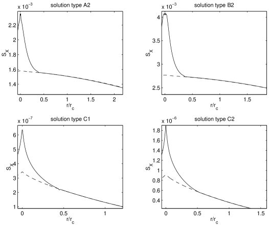
Figure 5.— Unconvolved X-ray profiles for the solution types A2 (upper left), B2 (upper right), C1 (lower left) and C2 (lower right), for cooling flow (solid line) and the corresponding cases of gas in hydrostatic equilibrium (dashed line). X-ray surface brightness in units of $erg~{}s^{-1}cm^{-2}ster^{-1}$ is plotted against ${{r}\over{r_{core}}}$. Individual plots have been magnified to highlight the differences between cooling flow and hydrostatic cases.

References

- (1)
- (2) Aghanim, N., De Luca, A., Bouchet, F. R., Gispert, R. & Puget, J. L., 1997, A & A, 325, 9
- (3) Allen, S. W., Fabian, A. C., Johnstone, R. M., Arnaud, K. A., & Nulsen, P. E. J., 1999 : astro-ph/9910188
- (4) Allen, S. W., 2000 : astro-ph/0002506
- (5) Barbosa, D., Bartlett, J. G., Blanchard, A. & Oukbir, J., 1996, astro-ph/9607036
- (6) Barbosa, D., Bartlett, J. G., Blanchard, A. & Oukbir, J., 1996, A & A, 314, 13
- (7) Bartlett, J. G. & Silk, J., 1994, ApJ, 423, 12
- (8) Bartlett, J. G., Blanchard, A. & Barbosa, D., astro-ph/9808308
- (9) Bartlett, J. G,. 2000 : astro-ph/0001267
- (10) Birkinshaw, M. & Hughes, J. P., 1994, ApJ, 420, 33
- (11) Birkinshaw, M. 1999, Phys Rep., 310, 97
- (12) Blanchard, A & Bartlett, J. G., 1998, A & A, 332, 49L
- (13) Cavaliere, A. & Fusco-Femiano, R., 1978, A & A, 70, 677
- (14) Evrard, A. E., 1990, ApJ, 363, 349
- (15) Fabian, A. C., Nulsen, P. E. J. & Canizares, C. R. 1984, Nature, 310, 733
- (16) Fabian, A. C. 1994, ARAA, 32, 277
- (17) Grego, L., Carlstrom, J. E., Joy, M. K., Reese, E. D., Holder, J. P., Patel, S., Cooray, A., & Holzapfel, W. L., 2000, : astro-ph/0003085
- (18) Herbig, T., Lawrence, C. R., Redhead, A. C. S., & Gulkis, S., 1995, ApJ, 449, L5
- (19) Holzapfel, W. L., et al. 1997, ApJ, 480, 449 Reese, E. D., 1999, preprint (astro-ph/9912010)
- (20) Hughes, J. P., & Birkinshaw, M., 1998, ApJ, 501, 1
- (21) Inagaki, Y., Suginohara, T. & Suto, Y., 1995, PASJ, 47, 411
- (22) Jaffe, W. 1980, ApJ, 241, 925
- (23) Jones, M. et al. 1993, Nature, 365, 320
- (24) Kellog, E., Baldwin, J. R. & Koch, D., 1975, ApJ, 199, 299
- (25) Komatsu, E., Kitayama, T., Suto, Y., Hattori, M., Kawabe, R., Matsuo, H., Schindler, S., & Yoshikawa, K., 1999, ApJ, 516, L1
- (26) Majumdar, S. & Subrahmanyan, R., 2000, MNRAS, 312, 724
- (27) Makino, N., Sasaki, S. & Suto, Y., 1998, ApJ, 497, 555
- (28) Markevitch, M., Forman, W. R., Sarazin, C. L. & Vikhlinin, A., 1998, ApJ, 504, 27
- (29) Mathews, W. G., & Bregman, J. N., 1978, ApJ, 224, 308
- (30) Navarro, J. F., Frenk, C. S., & White, S. D. M., 1997, ApJ, 40, 493
- (31) Oukbir, J. & Blanchard, A., 1992, A & A, 262, 21L
- (32) Oukbir, J. & Blanchard, A., 1997, A & A, 317, 1
- (33) Padmanabhan, T., 1993, Structure Formation in the Universe, Cambridge University Press, Cambridge
- (34) Peres, C. B., Fabian, A. C., Edge, A. C., Allen, A. W., Johnstone, R. M., & White, D. A., 1998, MNRAS, 298, 416
- (35) Pointecouteau, E., Giard, M., Benoit, A., Désert, F. X., Aghanim, N., Coron, N., Lamarre., J. A., & Delabrouille, J., 1999, ApJ, 519, L115
- (36) Press, W. H. & Schecter, P., 1974, ApJ, 187, 225
- (37) Reese, E. D., et al. 1999 : astro-ph/9912071
- (38) Rizza, E., Loken, C., Bliton, M., Roettiger, K., & Burns, J., 2000, ApJ, 119, 21
- (39) Roettiger, K., Stone, J. M. & Mushotzky, R. F., 1997, ApJ, 482, 588
- (40) Sarazin, C. L. 1986, Rev. Mod. Phys., 58, 1
- (41) Sarazin, C. L. & White, R. E. 1987, ApJ, 320, 32
- (42) Sarazin, C. L. & Graney, C. M. 1991, ApJ, 375, 532
- (43) Saunders, R. et al. 1999: astro-ph/9904168
- (44) Schlickeiser, R. 1991, A & A, 128, 23L
- (45) Schmutzler, T. & Tscharnuter, W. M. 1993, A & A, 273, 318
- (46) Silverberg, R. F. et al, 1997, ApJ, 485, 22
- (47) Soker, N. & Sarazin, C. L. 1988, ApJ, 327, 66
- (48) Subrahmanyan, R., Kesteven, M. J., Ekers, R. D., Sinclair, M. & Silk, J. 1998, MNRAS, 298, 1189
- (49) Sulkanen, M. E., Burns, J. O. & Norman, M. L. 1989, ApJ, 344, 604
- (50) Sunyaev, R. A. & Zel’dovich, Ya. B. 1972, Comm. Astrophys. Space Phys.,4, 173
- (51) Suto, Y., Sasaki, S. & Makino, Y., 1998, ApJ, 509, 544
- (52) Thomas, P., Fabian, A. C. & Nulsen, P.E.J. 1987, MNRAS, 228, 973.
- (53) Waxman, E. & Miralda-Escude’, J., 1995, ApJ, 451, 451
- (54) White, R. E., & Sarazin, C. L., 1987, ApJ, 318, 629
- (55) Wise, M. W. & Sarazin C. L., 1993, ApJ, 415, 58
- (56) Yoshikawa, K., Itoh, M. & Suto, Y., 1998, PASJ, 50, 203