Thermonuclear Explosions of Chandrasekhar-Mass White Dwarfs
Abstract
We present a new way of modeling turbulent thermonuclear deflagration fronts in Chandrasekhar-mass white dwarfs, consisting of carbon and oxygen, undergoing a type Ia supernova explosion. Our approach is a front capturing/tracking hybrid scheme, based on a level set method, which treats the front as a mathematical discontinuity and allows for full coupling between the front geometry and the flow field. First results of the method applied to the problem of type Ia supernovae are discussed. It will be shown that even in 2-D and even with a physically motivated sub-grid model numerically “converged” results are difficult to obtain.
keywords:
Hydrodynamics, turbulent combustion, type Ia supernovaeW. Hillebrandt et al. \titlerunningheadThermonuclear explosions
and
Dedicated to Joe Monaghan on the occasion of his 60th birthday
1 Introduction
Type Ia supernovae, i.e. stellar explosions which do not have hydrogen in their spectra, but intermediate-mass elements, such as silicon, calcium, cobalt, and iron, have recently received considerable attention because it appears that they can be used as “standard candles” to measure cosmic distances out to billions of light years away from us. Moreover, observations of type Ia supernovae seem to indicate that we are living in a universe that started to accelerate its expansion when it was about half its present age. These conclusions rest primarily on phenomenological models which, however, lack proper theoretical understanding, mainly because the explosion process, initiated by thermonuclear fusion of carbon and oxygen into heavier elements are difficult to simulate even on supercomputers, for reasons we shall discuss in this article.
The most popular progenitor model for the average type Ia supernovae is a massive white dwarf, consisting of carbon and oxygen, which approaches the Chandrasekhar mass, M M⊙, by a yet unknown mechanism, presumably accretion from a companion star, and is disrupted by a thermonuclear explosion (see, e.g., [52] for a review). Arguments in favour of this hypothesis include the ability of these models to fit the observed spectra and light curves.
However, not only is the evolution of massive white dwarfs to explosion very uncertain, leaving room for some diversity in the allowed set of initial conditions (such as the temperature profile at ignition), but also the physics of thermonuclear burning in degenerate matter is complex and not well understood. The generally accepted scenario is that explosive carbon burning is ignited either at the center of the star or off-center in a couple of ignition spots, depending on the details of the previous evolution. After ignition, the flame is thought to propagate through the star as a sub-sonic deflagration wave which may or may not change into a detonation at low densities (around 107g/cm3). Numerical models with parameterized velocity of the burning front have been very successful, the prototype being the W7 model of [38]. However, these models do not solve the problem because attempts to determine the effective flame velocity from direct numerical simulations failed and gave velocities far too low for successful explosions [27, 19, 1]. This has led to some speculations about ways to change the deflagration into a supersonic detonation [15, 16].
Numerical simulations of any kind of turbulent combustion have always been a challenge, mainly because of the large range of length scales involved. In type Ia supernovae, in particular, the length scales of relevant physical processes range from 10-3cm for the Kolmogorov-scale to several 107cm for typical convective motions. In the currently favored scenario the explosion starts as a deflagration near the center of the star. Rayleigh-Taylor unstable blobs of hot burnt material are thought to rise and to lead to shear-induced turbulence at their interface with the unburnt gas. This turbulence increases the effective surface area of the flamelets and, thereby, the rate of fuel consumption; the hope is that finally a fast deflagration might result, in agreement with phenomenological models of type Ia explosions [38].
Despite considerable progress in the field of modeling turbulent combustion for astrophysical flows (see, e.g., [34]), the correct numerical representation of the thermonuclear deflagration front is still a weakness of the simulations. Methods used up to now are based on for the reactive-diffusive flame model [17], which artificially stretches the burning region over several grid zones to ensure an isotropic flame propagation speed. However, the soft transition from fuel to ashes stabilizes the front against hydrodynamical instabilities on small length scales, which in turn results in an underestimation of the flame surface area and – consequently – of the total energy generation rate. Moreover, because nuclear fusion rates depend on temperature nearly exponentially, one cannot use the zone-averaged values of the temperature obtained this way to calculate the reaction kinetics.
The front tracking method described here cures some of these weaknesses. It is based on the so-called level set technique which was originally introduced by Osher and Sethian [39]. They used the zero level set of a -dimensional scalar function to represent -dimensional front geometries. Equations for the time evolution of such a level set which is passively advected by a flow field are given in [47]. The method has been extended to allow the tracking of fronts propagating normal to themselves, e.g. deflagrations and detonations [46]. In contrast to the artificial broadening of the flame in the reaction-diffusion-approach, this algorithm is able to treat the front as an exact hydrodynamical discontinuity.
In the following sections we present the main ideas and governing equations of this approach. We describe only the most simple implementation of the flame model and leave extensions including the reconstruction of the thermo-dynamical properties of mixed cells to subsequent papers. The main emphasis will be to demonstrate that the method can indeed be applied to the supernova problem. In addition, we will show that even if one attempts to model the physics of thermonuclear burning on unresolved scales well by physically motivated LES one still has to perform calculations with very high spatial resolution in order to be at least near to a converged solution.
The numerical results presented here were obtained by performing 2D simulations, but there is no problem extending them to 3D. Such simulations are under way.
2 General properties of exploding white dwarfs
To a very good approximation, the exploding white dwarf material can be described as a fully ionized plasma with varying degrees of electron degeneracy, satisfying the fluid approximation. The governing equations are the hydrodynamical equations for mass, species, momentum, and energy transport including gravitational acceleration, viscosity, heat and mass diffusion [24], and nuclear energy generation [2]. They must be supplemented by an equation of state for an ideal gas of nuclei, an arbitrarily relativistic and degenerate electron gas, radiation, and electron-positron pair production and annihilation [8]. The gravitational potential is calculated with the help of the Poisson equation. In numerical simulations that fully resolve the relevant length scales for dissipation, diffusion, and nuclear burning it is possible to obtain the energy generation rate from a nuclear reaction network (for a recent overview, see [49]) and the diffusion coefficients from an evaluation of the kinetic transport mechanisms [32]. If, on the other hand, these scales are unresolved – as is usually the case in simulations on scales of the stellar radius – subgrid-scale models are required to compute (or parameterize) the effective large-scale transport coefficients and burning rates, which are more or less unrelated to the respective microphysical quantities [19, 34].
Initial conditions can be obtained from hydrostatic spherically symmetric models of the accreting white dwarf or – for Chandrasekhar mass progenitors – from the Chandrasekhar equation for a fully degenerate, zero temperature white dwarf [21]. Given the initial conditions and symmetries specifying the boundary conditions, the dynamics of the explosion can in principle be determined by numerically integrating the equations of motion. [31] gives a detailed account of some current numerical techniques used for modeling supernovae.
2.1 Nuclear burning in degenerate C+O matter
Owing to the strong temperature dependence of the nuclear reaction rates, at K [13], nuclear burning during the explosion is confined to microscopically thin layers that propagate either conductively as subsonic deflagrations (“flames”) or by shock compression as supersonic detonations [7, 24]. Both modes are hydrodynamically unstable to spatial perturbations as can be shown by linear perturbation analysis. In the nonlinear regime, the burning fronts are either stabilized by forming a cellular structure or become fully turbulent – either way, the total burning rate increases as a result of flame surface growth [26, 50, 55]. Neither flames nor detonations can be resolved in explosion simulations on stellar scales and therefore have to be represented by numerical models.
When the fuel exceeds a critical temperature where burning proceeds nearly instantaneously compared with the fluid motions (see [48] for a suitable definition of ), a thin reaction zone forms at the interface between burned and unburned material. It propagates into the surrounding fuel by one of two mechanisms allowed by the Rankine-Hugoniot jump conditions: a deflagration (“flame”) or a detonation.
If the overpressure created by the heat of the burning products is sufficiently high, a hydrodynamical shock wave forms that ignites the fuel by compressional heating. Such a self-sustaining combustion front that propagates by shock-heating is called a detonation. If, on the other hand, the initial overpressure is too weak, the temperature gradient at the fuel-ashes interface steepens until an equilibrium between heat diffusion (carried out predominantly by electron-ion collisions) and energy generation is reached. The resulting combustion front consists of a diffusion zone that heats up the fuel to , followed by a thin reaction layer where the fuel is consumed and energy is generated. It is called a deflagration or simply a flame and moves subsonically with respect to the unburned material [24]. Flames, unlike detonations, may therefore be strongly affected by turbulent velocity fluctuations of the fuel. Only if the unburned material is at rest, a unique laminar flame speed can be found which depends on the detailed interaction of burning and diffusion within the flame region, e.g. [55]. Following [24], it can be estimated by assuming that in order for burning and diffusion to be in equilibrium, the respective time scales, and , where is the flame thickness and is the thermal diffusivity, must be similar: . Defining , one finds , where should be evaluated at [48]. This is only a crude estimate due to the strong -dependence of . Numerical solutions of the full equations of hydrodynamics including nuclear energy generation and heat diffusion are needed to obtain more accurate values for as a function of and fuel composition. Laminar thermonuclear carbon and oxygen flames at high to intermediate densities were investigated by [4, 14, 51], and, using a variety of different techniques and nuclear networks, by [48]. For the purpose of SN Ia explosion modeling, one needs to know the laminar flame speed cm s-1 for g cm-3, the flame thickness cm (defined here as the width of the thermal pre-heating layer ahead of the much thinner reaction front), and the density contrast between burned and unburned material (all values quoted here assume a composition of [48]). The thermal expansion parameter reflects the partial lifting of electron degeneracy in the burning products, and is much lower than the typical value found in chemical, ideal gas systems [50].
Observed on scales much larger than , the internal reaction-diffusion structure can be neglected and the flame can be approximated as a density jump that propagates locally with the normal speed . This “thin flame” approximation allows a linear stability analysis of the front with respect to spatial perturbations. The result shows that thin flames are linearly unstable on all wavelengths. It was discovered first by Landau (1944) [23] and Darrieus (1938) [10] and is hence called the “Landau-Darrieus” (LD) instability. Subject to the LD instability, perturbations grow until a web of cellular structures forms and stabilizes the front at finite perturbation amplitudes [54]. The LD instability therefore does not, in general, lead to the production of turbulence. In the context of SN Ia models, the nonlinear LD instability was studied by [3], using a statistical approach based on the Frankel equation, and by [33] employing 2D hydrodynamics and a one-step burning rate. Both groups concluded that the cellular stabilization mechanism precludes a strong acceleration of the burning front as a result of the LD instability. However, [3] mention the possible breakdown of stabilization at low stellar densities (i.e., high ) which is also indicated by the lowest density run of [33].
2.2 Hydrodynamic instabilities and turbulence
The best studied and probably most important hydrodynamical effect for modeling SN Ia explosions is the Rayleigh-Taylor (RT) instability resulting from the buoyancy of hot, burned fluid with respect to the dense, unburned material [29, 30, 27, 18, 19, 34], and after more than five decades of experimental and numerical work, the basic phenomenology of nonlinear RT mixing is fairly well understood [11, 25, 45, 42, 53]: Subject to the RT instability, small surface perturbations grow until they form bubbles (or “mushrooms”) that begin to float upward while spikes of dense fluid fall down. In the nonlinear regime, bubbles of various sizes interact and create a foamy RT mixing layer whose vertical extent grows with time according to a self-similar growth law, , where is a dimensionless constant () and is the background gravitational acceleration.
Secondary instabilities related to the velocity shear along the bubble surfaces [35] quickly lead to the production of turbulent velocity fluctuations that cascade from the size of the largest bubbles ( cm) down to the microscopic Kolmogorov scale, cm where they are dissipated [34, 19]. Since no computer is capable of resolving this range of scales, one has to resort to statistical or scaling approximations of those length scales that are not properly resolved. The most prominent scaling relation in turbulence research is Kolmogorov’s law for the cascade of velocity fluctuations, stating that in the case of isotropy and statistical stationarity, the mean velocity of turbulent eddies with size scales as [22]. Given the velocity of large eddies, e.g. from computer simulations, one can use this relation to extrapolate the eddy velocity distribution down to smaller scales under the assumption of isotropic, fully developed turbulence [34]. Knowledge of the eddy velocity as a function of length scale is important to classify the burning regime of the turbulent combustion front [37, 36, 20]. The ratio of the laminar flame speed and the turbulent velocity on the scale of the flame thickness, , plays an important role: if , the laminar flame structure is nearly unaffected by turbulent fluctuations. Turbulence does, however, wrinkle and deform the flame on scales where , i.e. above the Gibson scale defined by [40]. These wrinkles increase the flame surface area and therefore the total energy generation rate of the turbulent front [9]. In other words, the turbulent flame speed, , defined as the mean overall propagation velocity of the turbulent flame front, becomes larger than the laminar speed . If the turbulence is sufficiently strong, , the turbulent flame speed becomes independent of the laminar speed, and therefore of the microphysics of burning and diffusion, and scales only with the velocity of the largest turbulent eddy [9, 5]:
| (1) |
Because of the unperturbed laminar flame properties on very small scales, and the wrinkling of the flame on large scales, the burning regime where is called the corrugated flamelet regime [41, 5].
As the density of the white dwarf material declines and the laminar flamelets become slower and thicker, it is plausible that at some point turbulence significantly alters the thermal flame structure [20, 37]. This marks the end of the flamelet regime and the beginning of the distributed burning, or distributed reaction zone, regime, e.g. [41]. So far, modeling the distributed burning regime in exploding white dwarfs has not been attempted explicitely since neither nuclear burning and diffusion nor turbulent mixing can be properly described by simplified prescriptions. Phenomenologically, the laminar flame structure is believed to be disrupted by turbulence and to form a distribution of reaction zones with various lengths and thicknesses. In order to find the critical density for the transition between both regimes, we need to formulate a specific criterion for flamelet breakdown. A criterion for the transition between both regimes is discussed in [37, 36] and [20]:
| (2) |
Inserting the results of [48] for and as functions of density, and using a typical turbulence velocity cm s-1, the transition from flamelet to distributed burning can be shown to occur at a density of g cm-3 [36].
3 A numerical scheme for turbulent combustion
Our aim is now to convert some of the ideas presented in the previous Sections into a numerical scheme. The basic ingredients will be a finite-volume method to solve the fluid-dynamics equation, a front-tracking algorithm which allows us to propagate the thermonuclear flame (assumed to be in the flamelet regime), and a model to determine the turbulent velocity fluctuations on unresolved sub-grid scales.
3.1 The level set method
The central aspect of our front tracking method is the association of the front geometry (a time-dependent set of points ) with an isoline of a so-called level set function :
| (3) |
Since is not completely determined by this equation, we can additionally postulate that be negative in the unburnt and positive in the burnt regions, and that be a “smooth” function, which is convenient from a numerical point of view. This smoothness can be achieved, for example, by the additional constraint that in the whole computational domain, with the exception of possible extrema and kinks of . The ensemble of these conditions produces a which is a signed distance function, i.e. the absolute value of at any point equals the minimal front distance. The normal vector to the front is defined to point towards the unburnt material.
The task is now to find an equation for the temporal evolution of such that the zero level set of behaves exactly as the flame. Such an expression can be obtained by the consideration that the total velocity of the front consists of two independent contributions: it is advected by the fluid motions at a speed and it propagates normal to itself with a burning speed .
Since for deflagration waves a velocity jump usually occurs between the pre-front and post-front states, we must explicitly specify which state and refer to; traditionally, the values for the unburnt state are chosen. Therefore, one obtains for the total front motion
| (4) |
The total temporal derivative of at a point attached to the front must vanish, since is, by definition, always 0 at the front:
| (5) |
This leads to the desired differential equation describing the time evolution of :
| (6) |
This equation, however, cannot be applied on the whole computational domain, mainly because using this equation everywhere will in most cases destroy ’s distance function property. Therefore additional measures must be taken in the regions away from the front to ensure a “well-behaved” [44].
The situation is further complicated by the fact that the quantities and which are needed to determine are not readily available in the cells cut by the front. In a finite volume context, these cells contain a mixture of pre- and post-front states instead. Nevertheless one can assume that the conserved quantities (mass, momentum and total energy) of the mixed state satisfy the following conditions:
| (7) | |||||
| (8) | |||||
| (9) |
Here denotes the volume fraction of the cell occupied by the unburnt state. In order to reconstruct the states before and behind the flame, a nonlinear system consisting of the equations above, the Rankine-Hugoniot jump conditions and a burning rate law must be solved.
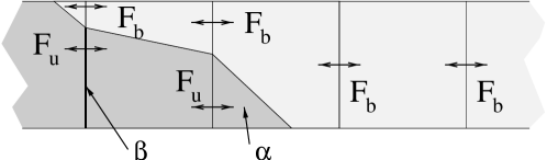
Having obtained the reconstructed pre- and post-front states in the mixed cells, it is not only possible to determine , but also to separately calculate the fluxes of burnt and unburnt material over the cell interfaces. Consequently, the total flux over an interface can be expressed as a linear combination of burnt and unburnt fluxes weighted by the unburnt interface area fraction (see Fig. 1):
| (10) |
3.2 Implementation
For our calculations, the front tracking algorithm was implemented as an additional module for the hydrodynamics code PROMETHEUS [12]. Here we describe a simple implementation of most of the ideas discussed in the previous section which we will call “passive implementation”. It assumes that the -function is advected by the fluid motions and by burning and is only used to determine the source terms for the reactive Euler equations. It must be noted that there exists no real discontinuity between fuel and ashes in this case; the transition is smeared out over about three grid cells by the hydro-dynamical scheme, and the level set only indicates where the thin flame front should be. However, the numerical flame is still considerably thinner than in the reaction-diffusion approach.
A complete implementation would contain in-cell-reconstruction and flux-splitting as proposed by [46] and outlined above. Therefore it should exactly describe the coupling between the flame and the hydrodynamic flow. This generalized version of the code has so-far only been applied to hydrogen combustion in air and, therefore, will be discussed elsewhere.
3.2.1 -Transport
Since the front motion consists of two distinct contributions, it is appropriate to use an operator splitting approach for the time evolution of . The advection term due to the fluid velocity reads in conservation form
| (11) |
[28]. This equation is identical to the advection equation of a passive scalar, like the concentration of an inert chemical species. Consequently, this contribution to the front propagation can be calculated by PROMETHEUS directly. The additional flame propagation due to burning is calculated at the end of each time step and a re-initialization of is done in order to keep it a signed distance function (see [44]).
3.2.2 Source terms
After the update of the level set function in each time step, the change of chemical composition and total energy due to burning is calculated in the cells cut by the front. In order to obtain these values, the volume fraction occupied by the unburnt material is determined in those cells by the following approach: from the value and the two steepest gradients of towards the front in - and -direction a first-order approximation of the level set function is calculated; then the area fraction of cell where can be found easily. Based on these results, the new concentrations of fuel, ashes and energy are obtained:
| (12) | ||||
| (13) | ||||
| (14) |
In principle this means that all fuel found behind the front is converted to ashes and the appropriate amount of energy is released. The maximum operator in eq. (12) ensures that no “reverse burning” (i.e. conversion from ashes to fuel) takes place in the cases where the average ash concentration is higher than the burnt volume fraction; such a situation can occur in a few rare cases because of unavoidable discretization errors of the numerical scheme.
3.3 Turbulent nuclear burning
The system of equations described so-far can be solved provided the normal velocity of the burning front is known everywhere and at all times. In our computations it is determined according to a flame-brush model of Niemeyer and Hillebrandt [34], which we will briefly outline for convenience.
As was mentioned before, nuclear burning in degenerate dense matter is believed to propagate on microscopic scales as a conductive flame, wrinkled and stretched by local turbulence, but with essentially the laminar velocity. Due to the very high Reynolds numbers macroscopic flows are highly turbulent and they interact with the flame, in principle down to the Kolmogorov scale. This means that all kinds of hydrodynamic instabilities feed energy into a turbulent cascade, including the buoyancy-driven Rayleigh-Taylor instability and the shear-driven Kelvin-Helmholtz instability. Consequently, the picture that emerges is more that of a “flame brush” spread over the entire turbulent regime rather than a wrinkled flame surface. For such a flame brush, the relevant minimum length scale is the so-called Gibson scale, defined as the lower bound for the curvature radius of flame wrinkles caused by turbulent stress. Thus, if the thermal diffusion scale is much smaller than the Gibson scale (which is the case for the physical conditions of interest here) small segments of the flame surface are unaffected by large scale turbulence and behave as unperturbed laminar flames (“flamelets”). On the other hand side, since the Gibson scale is, at high densities, several orders of magnitude smaller than the integral scale set by the Rayleigh-Taylor eddies and many orders of magnitude larger than the thermal diffusion scale, both transport and burning times are determined by the eddy turnover times, and the effective velocity of the burning front is independent of the laminar burning velocity.
A numerical realization of this general concept is presented in [34]. The basic assumption was that wherever one finds turbulence this turbulence is fully developed and homogeneous, i.e. the turbulent velocity fluctuations on a length scale are given by the Kolmogorov law , where is the integral scale, assumed to be equal to the Rayleigh-Taylor scale. Following the ideas outlined above, one can also assume that the thickness of the turbulent flame brush on the scale is of the order of itself. With these two assumptions and the definition of the Gibson scale one finds for
| (15) |
and , where defines , is the laminar burning speed and is the turbulent flame velocity on the scale .
In a second step this model of turbulent combustion is coupled to our finite volume hydro scheme. Since in every finite volume scheme scales smaller than the grid size cannot be resolved, we express in terms of the grid size , the (unresolved) turbulent kinetic energy , and the laminar burning velocity:
| (16) |
Here is determined from a sub-grid model [6, 34] and, finally, the effective turbulent velocity of the flame brush on scale is given by
| (17) |
with and , where is the local gravitational acceleration.
4 Application to the supernova problem
We have carried out numerical simulations in cylindrical rather than in spherical coordinates, mainly because it is much simpler to implement the level set on a Cartesian (r,z) grid. Moreover, the CFL condition is somewhat relaxed in comparison to spherical coordinates. The grid we used in most of our simulations maps the white dwarf onto 256256 mesh points, equally spaced for the innermost 226226 zones by =1.5106cm, but increasing by 10% from zone to zone in the outer parts. The white dwarf, constructed in hydrostatic equilibrium for a realistic equation of state, has a central density of 2.9109g/cm3, a radius of 1.5108cm, and a mass of 2.81033g, identical to the one used by [34]. The initial mass fractions of C and O are chosen to be equal, and the total binding energy turns out to be 5.41050erg. At low densities (g/cm3), the burning velocity of the front is set equal to zero because the flame enters the distributed regime and our physical model is no longer valid. However, since in reality some matter may still burn the energy release obtained in the simulations is probably somewhat too low.
 |
 |
 |
 |
Here we present only the results for two models, one in which nuclear burning was ignited off-center in a blob and a second one in which initially five blobs were burned as an initial condition, and refer to [43] for simulations with other initial conditions.
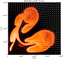
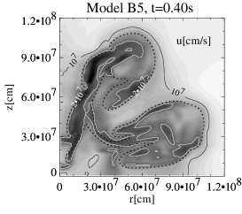
First, in Fig.2 a snapshot of the "five-blob" model B5 is shown at t = 0.4s. The leftt panel gives the position of the burning front, the temperatures (in gray-shading), and the expansion velocities. The rightpanel shows the distribution of turbulent velocity fluctuations. We find that, in accord with one’s intuition, most of the turbulence is generated in a very thin layer near the front. Since in the limit of high turbulence intensity the nuclear flames propagate with the turbulent velocity it is obvious that this propagation velocity exceeds the laminar flame speed. However, for most of the initial conditions we have investigated this increase was not sufficient to unbind the star. In fact, model B5 of [43] was the only one of the set that did explode.
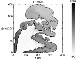
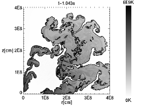
Moreover, we show the results obtained with 3 times higher resolution for comparison. Fig.3 gives a snapshot taken at 1.05s after ignition for the low-resolution run (left figure) and the high-resolution run, respectively. Although the increase in spatial resolution is only a factor of 3, the right panel shows clearly more structure. This is an important effect because in the flamelet regime the rate of fuel consumption, in first order, increases proportional to surface area of the burning front. The net effect is that the low-resolution model stays bound at the end of the computations, whereas the better resolved model explodes with an explosion energy of about 21050erg. Fig.3 also demonstrates that the level-set prescription allows to resolve the structure of the burning front down almost to the grid scale, thus avoiding artificial smearing of the front which is an inherent problem of front-capturing schemes. We want to stress that this gain of accuracy is not obtained at the expense of smaller CFL time steps because in our hybrid scheme the hydrodynamics is still done with cell-averaged quantities.
5 Conclusions
In this article, we have discussed the physics of thermonuclear combustion in degenerate dense matter of C+O white dwarfs. It was argued that not all relevant length-scales of this problem can be numerically resolved and, therefore, we have presented a numerical model to describe deflagration fronts with a reaction zone much thinner then the cells of the computational grid. The new approach was applied to the simulate thermonuclear supernova explosions. Our code works in 2 and 3 dimensions, but has only been used so far in 2D.
An implicit assumption of our numerical model is that on the resolved scales the flows are turbulent allowing us to describe the physics on the unresolved scales by a sub-grid model, in the spirit of large-eddy simulations. The results presented here indicate that for supernova simulations this assumption is still not satisfied if (in 2D and cylindrical coordinates) we use a 256 256 grid. In fact, we could demonstrate that for a particular set of initial conditions increasing the numerical resolution by a factor of 3 only changes a model that remains bound after most of the nuclear fuel was burnt into a, although weak, explosion. The reason is simply that more structure on small length scales increases the rate of fuel consumption and we suspect that even our better resolved simulation does not yet give the final answer, pushing even 2D supernova simulation to the limits of what can be done on present supercomputers.
The numerical scheme outlined in this paper can, of course, also be applied to chemical combustion in the flamelet regime and first successful attempts to model hydrogen combustion in air have already been made [46, 44]. Its advantage is always that it resolves the flame-front down to the grid-scale without making the time-steps intolerably small.
This work was supported in part by the Deutsche Forschungsgemeinschaft under Grant Hi 534/3-1, the DAAD, and by DOE under contract No. B341495 at the University of Chicago. The computations were performed at the Rechenzentrum Garching on a Cray J90.
References
- [1] W. D. Arnett and E. Livne. ApJ, 427:31, 1994.
- [2] W. David Arnett. Supernovae and Nucleosynthesis. Princeton University Press, Princeton, 1996.
- [3] S. I. Blinnikov and P. V. Sasorov. Phys. Rev. E, 53:4827, 1996.
- [4] J. R. Buchler, S. A. Colgate, and T. J. Mazurek. Journal de Physique, 41:, 1980.
- [5] P. Clavin. Annual Rev. Fluid Mech., 26:321, 1994.
- [6] M. J. Clement. ApJ, 406:651, 1993.
- [7] R. Courant and K. O.. Friedrichs. Supersonic Flow and Shock Waves. Springer, New York, 1948.
- [8] J. P. Cox and R. T. Giuli. Principles of Stellar Structure, Vol. II. Gordon and Breach, New York, 1968.
- [9] G. Damköhler. Z. Elektrochem., 46:601, 1940.
- [10] G. Darrieus. La Technique Moderne, 1944.
- [11] E. Fermi. In E. Segre, editor, Collected Works of Enrico Fermi, pages 816–821. 1951.
- [12] B. A. Fryxell, E. Müller, and W. D. Arnett. MPA Preprint, 449, 1989.
- [13] C. J. Hansen and S. D. Kawaler. Stellar Interiors. Springer, New York, 1994.
- [14] L. N. Ivanova, V. S. Imshennik, and V. M. Chechetkin. Pis ma Astronomicheskii Zhurnal, 8:17, 1982.
- [15] A. M. Khokhlov. A&A, 245:114, 1991.
- [16] A. M. Khokhlov. A&A, 245:L25, May 1991.
- [17] A. M. Khokhlov. ApJL, 419:L77, 1993.
- [18] A. M. Khokhlov. ApJL, 424:L115, 1994.
- [19] A. M. Khokhlov. ApJ, 449:695, 1995.
- [20] A. M. Khokhlov, E. S. Oran, and J. C. Wheeler. ApJ, 478:678, 1997.
- [21] Rudolf Kippenhahn and Alfred Weigert. Stellar Structure and Evolution. Springer, Berlin, 1989.
- [22] A. N. Kolmogorov. Dokl. Akad. Nauk SSSR, 30:299, 1941.
- [23] L. D. Landau. Acta Physicochim. URSS, 19:77, 1944.
- [24] L. D. Landau and E. M. Lifshitz. Fluid Mechanics. Butterworth-Heinemann, xxx, 1995.
- [25] D. Layzer. ApJ, 122:1, 1955.
- [26] B. Lewis and G. von Elbe. Combustion, Flames, and Explosions of Gases. Academic Press, New York, 2nd edition, 1961.
- [27] E. Livne. ApJL, 406:L17, 1993.
- [28] W. Mulder, S. Osher, and J. A. Sethian. JCP, 100:209, 1992.
- [29] E. Müller and W. D. Arnett. ApJL, 261:L109, 1982.
- [30] E. Müller and W. D. Arnett. ApJ, 307:619, 1986.
- [31] E. Müller. Simulation of astrophysical fluid flow. In O. Steiner and A. Gautschy, editors, Computational Methods for Astrophysical Fluid Flow, pages 343, Berlin, New York, 1998. Springer.
- [32] R. Nandkumar and C. J. Pethick. MNRAS, 209:511, 1984.
- [33] J. C. Niemeyer and W. Hillebrandt. ApJ, 452:779, 1995.
- [34] J. C. Niemeyer and W. Hillebrandt. ApJ, 452:769, 1995.
- [35] J. C. Niemeyer and W. Hillebrandt. Microscopic and macroscopic modeling of thermonuclear burning fronts. In P. Ruiz-Lapuente, R. Canal, and J. Isern, editors, Thermonuclear Supernovae, pages 441–456, Dordrecht, 1997. Kluwer.
- [36] J. C. Niemeyer and A. R. Kerstein. Burning regimes of nuclear flames in sn ia explosions. New Astronomy, 2:239, 1997.
- [37] J. C. Niemeyer and S. E. Woosley. ApJ, 475:740, 1997.
- [38] K. Nomoto, F. K. Thielemann, and K. Yokoi. ApJ, 286:644, 1984.
- [39] S. Osher and J. A. Sethian. JCP, 79:12, 1988.
- [40] N. Peters. In Symp. (Int.) Combust., 21st, pages 1232, Pittsburgh, 1988. Combustion Institute.
- [41] S. B. Pope. Annual Rev. Fluid Mech., 19:237, 1990.
- [42] K. I. Read. Physica D, 12:45, 1984.
- [43] M. Reinecke, W. Hillebrandt, and J. C. Niemeyer. A&A, 347:739, 1999.
- [44] M. Reinecke, W. Hillebrandt, J. C. Niemeyer, R. Klein, and A. Gröbl. A&A, 347:724, 1999.
- [45] D. H. Sharp. Physica D, 12:3, 1984.
- [46] V. Smiljanovski, V. Moser, and R. Klein. Combust. Theory Modelling, 1:183, 1997.
- [47] M. Sussman, P. Smereka, and S. Osher. JCP, 114:146, 1994.
- [48] F. X. Timmes and S. E. Woosley. ApJ, 396:649, 1992.
- [49] F. X. Timmes. ApJ Suppl., 124:241, 1999.
- [50] F. A. Williams. Combustion Theory. Benjamin/Cummings, Menlo Park, 2nd edition, 1985.
- [51] S. E. Woosley and T. A. Weaver. The physics of supernovae. In Dimitri Mihalas and Karl-Heinz A. Winkler, editors, Radiation Hydrodynamics in Stars and Compact Objects, Lecture Notes in Physics, volume 255, pages 91, Berlin, 1986. Springer.
- [52] S. E. Woosley. Type Ia supernovae: Carbon deflagration and detonation. In A. G. Petschek, editor, Supernovae, pages 182, Berlin, 1990. Springer.
- [53] D. L. Youngs. Physica D, 12:32, 1984.
- [54] Y. B.. Zeldovich. J. Appl. Mech. and Tech. Phys., 7:68, 1966.
- [55] Y. B. Zeldovich, G. I. Barenblatt, V. B. Librovich, and G. M. Makhviladze. The Mathematical Theory of Combustion and Explosions. Plenum, New York, 1985.