HIGH-REDSHIFT GALAXIES IN COLD DARK MATTER MODELS

Abstract

We use hydrodynamic cosmological simulations to predict the star formation properties of high-redshift galaxies ($z=2-6$) in five variants of the inflationary cold dark matter scenario, paying particular attention to $z=3$, the redshift of the largest “Lyman-break galaxy” (LBG) samples. Because we link the star formation timescale to the local gas density, the rate at which a galaxy forms stars is governed mainly by the rate at which it accretes cooled gas from the surrounding medium. At $z=3$, star formation in most of the simulated galaxies is steady on $\sim 200$ Myr timescales, and the instantaneous star formation rate (SFR) is correlated with total stellar mass. However, there is enough scatter in this correlation that a sample selected above a given SFR threshold may contain galaxies with a fairly wide range of masses. The redshift history and global density of star formation in the simulations depend mainly on the amplitude of mass fluctuations in the underlying cosmological model. The three models whose mass fluctuation amplitudes agree with recent analyses of the Ly$\alpha$ forest also reproduce the observed luminosity function of LBGs reasonably well, though the dynamic range of the comparison is small and the theoretical and observational uncertainties are large. The models with higher and lower amplitudes appear to predict too much and too little star formation, respectively, though they are not clearly ruled out. The intermediate amplitude models predict SFR$\;\sim 30-40M_{\odot}\;{\rm yr}^{-1}$ for galaxies with a surface density $\sim 1\;{\rm arcmin}^{-2}$ per unit redshift at $z=3$. They predict much higher surface densities at lower SFR, and significant numbers of galaxies with SFR$\;>10M_{\odot}\;{\rm yr}^{-1}$ at $z\geq 5$.

1 Introduction

The discovery and characterization of “Lyman-break” galaxies (LBGs) has opened a new window on the high-redshift universe, revealing a population of star-forming galaxies at $z>3$ whose comoving space density exceeds that of $L_{*}$ galaxies today (Steidel et al., 1996; Lowenthal et al., 1997). These galaxies can be identified by their unusual colors in deep imaging surveys because the intrinsic continuum break at $\lambda\sim 912$Å and the intergalactic absorption by the Ly$\alpha$ forest at $\lambda<1216$Å redshift into optical bands. Spectroscopic follow-up shows that photometry of Lyman-break objects yields robust approximate redshifts. From an optical imaging survey, one can therefore construct a sample of high-$z$ galaxies limited primarily by rest-frame ultraviolet (UV) luminosity, which, in the absence of dust extinction, is itself determined mainly by the instantaneous formation rate of massive stars. Application of this approach to the Hubble Deep Field (HDF; Williams et al., 1996) and other deep imaging surveys has yielded first attempts at one of the long-standing goals of observational cosmology, determination of the star formation history of the universe (e.g., Madau et al., 1996; Madau, 1997; Connolly et al., 1997; Steidel et al., 1999).

In this paper, we examine the ability of models based on inflation and cold dark matter (CDM) to account for the observed population of LBGs, using cosmological simulations that incorporate gravity, gas dynamics, and star formation. We consider five variants of the CDM scenario: three $\Omega_{m}=1$ models, a spatially flat low density model with a cosmological constant, and an open universe low density model with $\Omega_{\Lambda}=0$. The spatial clustering of the high-redshift galaxies in these simulations was discussed by Katz, Hernquist, & Weinberg (1999); here we focus on the masses and star formation properties of these galaxies.

Numerical simulations play two overlapping but distinct roles in cosmological studies. First, they provide quantitative predictions that can be compared to observations in order to test the underlying cosmological models. Second, they provide greater understanding of the observational phenomena themselves, by showing how observable structures might arise and evolve in a given cosmological scenario. In this paper we will emphasize the second of these roles, mainly because the numerical limitations of the simulations and our limited knowledge of the physics of star formation contribute uncertainties that are comparable to the differences between cosmological models. The examination of different cosmologies is still a useful exercise, however, because it shows how cosmological parameters and properties of primordial mass fluctuations affect the properties of the high-redshift galaxy population when other physical and numerical parameters are held fixed.

Hydrodynamic simulations complement the main alternative approach to the theoretical study of high-redshift galaxies, based on semi-analytic models of galaxy formation (e.g., Baugh et al., 1998; Kauffman et al., 1999; Somerville, Primack, & Faber, 2000). Semi-analytic models have the advantages of simplicity, flexibility, and speed. The price is a substantial number of approximations and tunable parameters; the values of some parameters are fixed by matching selected observations, leaving other observables as predictions of the model. Semi-analytic models incorporate simplified descriptions of gravitational collapse, mergers, and cooling of gas within dark halos. The strength of numerical simulations is their more realistic treatment of these processes. The only free parameters (apart from the physical parameters of the cosmological model being studied) are those related to the treatment of star formation and feedback. Given these parameters, simulations provide straightforward, untunable predictions. However, the simulation approach must contend with the numerical uncertainties caused by finite volume and finite resolution, and computational expense makes it a slow way to explore parameter space. Over the next few years, interactions between the numerical and semi-analytic approaches should strengthen both. Here we mainly present the numerical results on their own terms, with a brief comparison to interpretations based on semi-analytic models in §5.

We describe our numerical methods, treatment of star formation, and choice of cosmological model in §2. In §3 we present results for the LCDM model (CDM with a cosmological constant) at $z=3$, the redshift best probed by recent Lyman-break galaxy surveys. In §4 we broaden our scope, examining predictions of five different CDM models for the population of star-forming galaxies from $z=6$ to $z=2$. We discuss our results and prospects for future progress in §5.

2 Simulations

2.1 Numerical Parameters and Star Formation

All of our simulations use TreeSPH (Hernquist & Katz, 1989; Katz, Weinberg & Hernquist, 1996, hereafter KWH), a code that combines smoothed particle hydrodynamics (SPH; see Lucy, 1977; Gingold & Monaghan, 1977; Monaghan, 1992) with a hierarchical tree algorithm (Barnes & Hut, 1986) for computing gravitational forces. The method and illustrative cosmological applications are described in detail by KWH, so here we just specify the simulation parameters and recap the points that are most important to the present investigation.

Each of our simulations uses $64^{3}$ dark matter and $64^{3}$ SPH particles to model a triply periodic volume $11.111h^{-1}\;{\rm Mpc}$ comoving Mpc on a side, where $h\equiv H_{0}/(100\;{\rm km}\;{\rm s}^{-1}\;{\rm Mpc}^{-1})$. The simulations are evolved to $z=2$. For the three critical density ($\Omega_{m}=1$) cosmological models, the dark matter particle mass is $2.76\times 10^{9}M_{\odot}$ and the SPH particle mass is $1.45\times 10^{8}M_{\odot}$. For the two low density ($\Omega_{m}=0.4$) models, the dark matter particle mass is $8.27\times 10^{8}M_{\odot}$ and the SPH particle mass is $6.71\times 10^{7}M_{\odot}$. Gravitational forces are softened using a cubic spline kernel with a softening length $\epsilon=5h^{-1}\;{\rm kpc}$, equivalent to $\epsilon\approx 3.5h^{-1}\;{\rm kpc}$ for a Plummer softening law. The gravitational softening length is held fixed in comoving units, i.e., $\epsilon=1.25\;h^{-1}$ physical kpc at $z=3$. Particles have individual time steps that satisfy the conditions $\Delta t<0.4{\rm min}(\epsilon/|{\bf v}|,\sqrt{\epsilon/|{\bf a}|})$, where ${\bf v}$ is the peculiar velocity and ${\bf a}$ is the acceleration. SPH particle time steps are also required to satisfy the Courant condition (see KWH). The maximum time step for any particle is $\Delta t_{d}=H_{0}^{-1}/6000$.

Radiative cooling is computed assuming primordial composition gas with helium abundance $Y=0.24$ by mass. All of the simulations incorporate a photoionizing UV background with the spectral shape and redshift history computed by Haardt & Madau (1996), but with intensity reduced by a factor of two in order to approximately match the mean opacity of the Ly$\alpha$ forest given our assumed baryon density (Croft et al., 1997). In practice, the photoionizing background has negligible effect on the Lyman-break galaxy population, at least in the mass range that our simulations can resolve (Weinberg, Hernquist & Katz, 1997a).

The gas that resides in collapsed dark matter halos exhibits a two-phase structure: hot gas at roughly the halo virial temperature with a density profile similar to that of the dark matter (but exhibiting a core at small radii), and radiatively cooled gas with $T\sim 10^{4}\;{\rm K}$ at much higher overdensity. In simulations that do not incorporate star formation, the clumps of radiatively cooled gas have masses and sizes comparable to the luminous regions of observed galaxies. Our star formation algorithm is essentially a prescription for turning this dense, cold gas into collisionless stars, returning energy from supernova feedback to the surrounding medium. We provide a brief synopsis of this algorithm here and refer the reader to KWH for details.

An SPH gas particle is “eligible” to form stars if it is Jeans unstable, resides in a region of converging flow, has an overdensity $\rho_{g}/\overline{\rho_{g}}>55.7$ (corresponding to the virial boundary of a singular isothermal sphere in the spherical collapse model), and has a hydrogen number density exceeding $0.1\;{\rm cm}^{-3}$ (physical units). In practice, it is the physical density threshold that matters — gas with this density almost always satisfies the other criteria, except at very high redshift, where the overdensity threshold ensures that star formation does not occur in uncollapsed regions simply because the cosmic mean density is high. Once a gas particle is eligible to form stars, its star formation rate is given by

$${d\rho_{\star}\over dt}=-{d\rho_{g}\over dt}={c_{\star}\epsilon_{\star}\rho_{g}\over t_{g}},$$ (1)

or

$${d\ln\rho_{g}\over dt}=-{c_{\star}\epsilon_{\star}\over t_{g}},$$ (2)

where $c_{\star}$ is a dimensionless star formation rate parameter, $\epsilon_{\star}$ is the fraction of the particle’s gas mass that will be converted to stellar mass in a single simulation timestep, and the gas flow timescale $t_{g}$ is the maximum of the local gas dynamical time, $t_{\rm dyn}=(4\pi G\rho_{g})^{-1/2}$, and the local cooling time. Each SPH particle has both a gas mass and a stellar mass (initially zero); the total gas$+$stellar mass contributes to gravitational forces, but only the gas mass is used in computing the SPH properties and forces. The probability $p$ that an eligible SPH particle undergoes a star formation event in an integration timestep of duration $\Delta t$ is

$$p=1-\exp\left({-c_{*}\Delta t\over t_{g}}\right),$$ (3)

and if the particle does undergo such an event then $\epsilon_{\star}=1/3$ of its remaining gas mass is converted into stars during that step. In the limit (nearly always satisfied in the simulations) that $c_{*}\Delta t/t_{g}\ll 1$, this algorithm yields the average star formation rate given by equation (1). Once a particle’s gas mass falls below 5% of its original mass, it is converted into a collisionless, pure star particle, affected only by gravity, and its residual gas mass is redistributed to its SPH neighbors.

When an SPH particle undergoes star formation, recycled gas and supernova feedback energy are distributed to the particle and its neighbors, assuming a Miller-Scalo (1979) initial mass function truncated at $0.1M_{\odot}$ and $100M_{\odot}$ and $10^{51}$ ergs per supernova. This feedback energy is usually radiated away because it is released into a dense, gas rich medium with a short cooling time. Feedback therefore has only a modest impact in our simulations, and this is the physically appropriate result if the proto-galactic interstellar medium is fairly smooth and as dense as our simulations imply. It is possible that strong inhomogeneities in the interstellar medium (on scales well below our resolution limits) allow feedback to have a stronger effect in real proto-galaxies, and explicit modeling of this possibility is an important direction for future investigation. The scenario that we investigate here is a physically plausible limiting case.

In all of our simulations we set the star formation rate parameter $c_{\star}$ to 0.1 and $\epsilon_{\star}$ to 1/3. As shown in KWH, the stellar masses of the simulated galaxies are insensitive to the value of $c_{\star}$. In the KWH tests, an order of magnitude increase to $c_{\star}=1.0$ changes the total stellar mass in the box at $z=2$ by only 15%, and the effect of a higher $c_{\star}$ is actually to decrease the stellar mass because star formation occurs in lower density gas where supernova feedback can have a stronger effect. Indeed, one obtains nearly the same galaxy population in simulations that do not include star formation at all, except that in this case the “galaxies” are the clumps of cold, dense gas instead of the clumps of cold, dense gas and stars (see KWH, figure 5). In our simulations, the rate at which a galaxy forms stars is governed mainly by the rate at which gas condenses from the hot halo into the cold clump; the regulation implied by equation (1) ensures that the gas condensation rate and the star formation rate cannot get too far out of step. The link between star formation rate and gas density is physically motivated, since denser gas is more gravitationally unstable and more easily able to radiate its energy. In the case where the cooling timescale is short and $t_{g}=t_{\rm dyn}$, equation (1) implies $\dot{\rho}_{*}\propto\rho_{g}^{3/2}$, similar to the Schmidt-law $\dot{\rho}_{*}\propto\Sigma_{g}^{3/2}$ observed to hold over a large dynamic range in a wide variety of local galaxies (Schmidt, 1959; Kennicutt, 1998).

2.2 Cosmological Models

We consider five different cosmological models, all of which assume Gaussian primordial fluctuations and a universe dominated by cold, collisionless dark matter. In all cases we adopt a baryon density parameter $\Omega_{b}=0.0125h^{-2}$ based on Walker et al. (1991), though a higher $\Omega_{b}$ is suggested by recent analyses of the Ly$\alpha$ forest opacity (Rauch et al., 1997; Weinberg et al., 1997b) and the deuterium abundance in high-redshift Lyman limit systems (Burles & Tytler 1997, 1998). The model we refer to as “standard” CDM (SCDM) assumes $\Omega_{m}=1$, $h=0.5$, and an rms linear theory fluctuation in $8h^{-1}\;{\rm Mpc}$ spheres of $\sigma_{8}=0.7$. For this model we use the parameterization of the CDM power spectrum given by Bardeen et al. (1986). The $\sigma_{8}=0.7$ normalization is roughly consistent with the observed abundance of rich galaxy clusters (White, Efstathiou, & Frenk, 1993), but the SCDM model does not reproduce the amplitude of cosmic microwave background anisotropies observed by the COBE-DMR experiment (Smoot et al., 1992; Bennett et al., 1996). Our second model, COBE-normalized CDM (CCDM), is the same as SCDM except that the normalization $\sigma_{8}=1.2$ is chosen to match the 4-year COBE data (Gorski et al. 1996; see Bunn & White 1997 for a discussion of the CDM normalization). With this value of $\sigma_{8}$ and $\Omega_{m}=1$, the CCDM model produces galaxy clusters that are too massive to be consistent with observations.

One way to reconcile the COBE-DMR anisotropies and the observed cluster abundance within the context of $\Omega_{m}=1$ CDM models is to assume that inflation generates a primeval power spectrum that is “tilted” instead of scale-invariant, $P(k)\propto k^{n}$ with $n<1$. For our tilted CDM (TCDM) model, we adopt $n=0.80$ and the transfer function given by equation (D28) of Hu & Sugiyama (1996), which treats baryon damping effects more accurately than the original Bardeen et al. (1986) formulation. We normalize this analytic fit to the power spectrum to the amplitude $\sigma_{8}=0.54$ implied by COBE normalization, which we compute using the CMBFAST code of Seljak & Zaldarriaga (1996; Zaldarriaga, Seljak, & Bertschinger 1998), assuming the standard tensor mode contribution to microwave background anisotropies predicted by power law inflation models.

Another way to resolve the COBE/cluster conflict is to lower the value of $\Omega_{m}$, reducing cluster masses for a given $\sigma_{8}$. We consider two different low-$\Omega_{m}$ CDM models, one (LCDM) with a spatially flat universe and a cosmological constant $\Omega_{\Lambda}=1-\Omega_{m}$ and one (OCDM) with an open universe and $\Omega_{\Lambda}=0$. For LCDM we adopt $\Omega_{m}=0.4$, $h=0.65$, and a primeval spectral index $n=0.93$. With the tensor mode contribution, CMBFAST implies a normalization $\sigma_{8}=0.8$, which provides a good match to the cluster abundances for $\Omega_{m}=0.4$ (White, Efstathiou, & Frenk, 1993). We again use the Hu & Sugiyama (1996) formulation of the transfer function. For OCDM, we adopt $\Omega_{m}=0.4$, $h=0.65$, $n=1.0$, and a 2-year COBE-DMR normalization $\sigma_{8}=0.75$ (Ratra et al., 1997). Cluster masses in this model are lower than those in TCDM or LCDM, but they are consistent with current observations given their uncertainties (Cole et al., 1997). For OCDM we use the transfer function of Efstathiou, Bond, & White (1992) with $\Gamma=0.234$; the Hu & Sugiyama (1996) formulation is more accurate, but we were unaware of it at the time we ran the OCDM simulation. In practice, the differences between different analytic or numerical formulations of transfer functions are of the same magnitude as the changes caused by slight shifts in the adopted values of $h$, $\Omega_{b}$, or $\Omega_{m}$.

Parameters of the five cosmological models are listed in Table 1. Figure 1 shows the linear theory power spectra of the five models, over the range of scales represented in the initial conditions of our simulations. Instead of $P(k)$ itself, we plot $\Delta^{2}(k)\equiv 4\pi k^{3}P(k)$, which (with our Fourier transform convention) is the contribution to the variance of linear mass fluctuations per unit interval of ln$k$ (see Peacock & Dodds, 1994). The differences in fluctuation amplitude among the three $\Omega_{m}=1$ models are easy to see, as is the difference in $P(k)$ shape between the CCDM/SCDM models and the tilted (TCDM) and low density (OCDM/LCDM) models. Although LCDM has a slightly higher normalization than OCDM at $z=0$ ($\sigma_{8}=0.80$ vs. $\sigma_{8}=0.75$), OCDM has higher amplitude fluctuations at $z=3$ because of the smaller ratio of linear growth factors between $z=3$ and $z=0$ in an open universe.

Figure 1: Amplitude of linear mass fluctuations in the different cosmological models at $z=3$. The quantity $\Delta^{2}(k)\equiv 4\pi k^{3}P(k)$ is the contribution to the variance of fluctuations per unit interval of $\ln k$. The wavenumber $k$ is in comoving $h\;{\rm Mpc}^{-1}$. The range shown is from the fundamental mode of the simulation cube, $k_{f}=2\pi/(11.111h^{-1}\;{\rm Mpc})$, to the Nyquist frequency of the initial particle grid, $k_{N}=32k_{f}$.

3 Lyman-Break Galaxies in the LCDM Model

We will focus in this Section on the galaxy population of the LCDM model at $z=3$, then turn to other models and other redshifts in §4. Figure 2 shows particle distributions at $z=3$ from the full $11.111h^{-1}\;{\rm Mpc}$ simulation cube (top panels) and a $0.09h^{-1}\;{\rm Mpc}$ subcube containing the richest concentration of galaxies (bottom panels). The top panels show numerous concentrations of dense, shock heated gas, with typical temperatures $T\sim 10^{6}\;{\rm K}$ corresponding to the virial temperatures of the corresponding dark matter halos. However, the zoomed view at the lower left reveals the two phase structure that characterizes collapsed regions of the simulation. Extremely overdense clumps of $10^{4}\;{\rm K}$ gas, typically a few kpc in size, reside in a background of gas with $T\gtrsim 10^{6}\;{\rm K}$. These dense concentrations of cold gas are, of course, the sites of star formation, as shown in the lower right panel. Because the knots of cold gas and stars stand out so clearly from the background, there is no ambiguity in identifying the galaxies in such a simulation; one only needs an algorithm that picks out these clumps. We use the SKID algorithm (Spline-Kernel Interpolated DENMAX; see KWH and Gelb & Bertschinger 1994), as implemented by Stadel, Katz, & Quinn, which identifies clumps of gravitationally bound particles associated with a common density maximum.

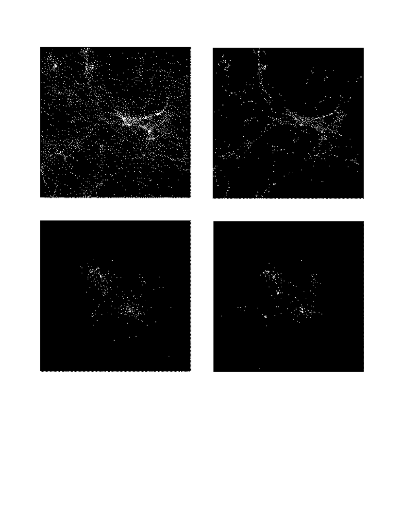
Figure 2: Gas and galaxies in the LCDM simulation at $z=3$. Upper panels show the gas distribution in the full $11.111h^{-1}\;{\rm Mpc}$ simulation cube (comoving size), color-coded by $\log T$ (left) and by $\log\rho_{g}$ (right). The lower left panel shows the gas temperature in a cubical sub-volume $0.09h^{-1}\;{\rm Mpc}$ (comoving) on a side. The lower right panel shows the dark matter (blue), gas (red) and star (yellow) particles in the same sub-volume. The temperature scale in the left hand panels runs from several thousand K (blue) to $10^{4}\;{\rm K}$ (magenta), $10^{5}\;{\rm K}$ (orange/yellow), and $\geq 10^{6}\;{\rm K}$ (white). Color GIF file provided separately on astro-ph.

In collapsing dark matter halos that contain a small number of particles, the resolution of the SPH calculation becomes too low for the simulation to follow the cooling of the gas and subsequent star formation. Gardner et al. (1997, 2000) find that simulated halos with at least 60 dark matter particles nearly always contain a cold gas concentration, while halos with fewer particles often do not. We can therefore resolve the existence of galaxies in halos with mass $M>60m_{\rm dark}$, a quantity that we list in Table 1 as an indication of our dark matter mass resolution. At $z=3$, the halo circular velocity corresponding to this limiting mass (plus the associated baryon mass) is $v_{c}\sim 140\;{\rm km}\;{\rm s}^{-1}$ in the $\Omega_{m}=1$ models and $v_{c}\sim 95\;{\rm km}\;{\rm s}^{-1}$ in the low density models (see Gardner et al. 1997, equation 3). Comparison of LCDM simulations with $64^{3}$ and $128^{3}$ SPH particles in the same $11.111h^{-1}\;{\rm Mpc}$ volume (Gardner et al., in preparation; Aguirre et al., in preparation) suggests that the requirement for accurate estimation of a galaxy’s star formation rate via equation (1) is somewhat more stringent, corresponding to 60 or more particles in the condensed baryon phase (cold gas plus stars). We list $60m_{\rm SPH}$ as an approximate baryon mass resolution limit for star formation calculations in Table 1.

Figure 3: Dependence of star formation rate (SFR) on time-averaging, for simulated galaxies in the LCDM model at $z=3$. The $x$-axis is the galaxy star formation rate averaged over $\Delta t=200$ Myr. Open circles show the instantaneous star formation rate, estimated by applying the prescription of §2 (see eq. 1) to the simulated gas distribution. Asterisks show the star formation rate averaged over $\Delta t=20$ Myr. Points along the axis have SFR $<0.1M_{\odot}/$yr. The age of the universe at this redshift is 1.97 Gyr.

For the galaxies at $z=3$, the asterisks in Figure 3 compare the star formation rate averaged over the previous 20 Myr to the star formation rate averaged over the previous 200 Myr. The two rates are usually within a factor of two of each other and are often much closer, indicating that star formation in our simulated galaxies is fairly steady over intervals of 200 Myr. Circles in Figure 3 show the “instantaneous” star formation rate calculated by applying the prescription of §2 to the gas particle distribution. This is the rate that would be used to calculate star formation in the simulation’s next system timestep (of duration $\Delta t=2.5$ Myr). The tight correlation between this estimate of the star formation rate and the rates averaged over longer intervals demonstrates that the instantaneous estimate is not sensitive to numerical “noise” in particle densities and positions, at least for systems with star formation rate $>1M_{\odot}/$yr. We will henceforth use the instantaneous estimate as our standard measure of the star formation rate (hereafter denoted SFR), with Figure 3 as evidence that our results are insensitive to this choice.

Figure 4: Correlation between instantaneous star formation rate and stellar mass, for simulated galaxies in the LCDM model at $z=3$. The solid line shows the relation SFR=$M_{*}/t$ that would apply for galaxies forming stars at a constant rate over the age of the universe $t=1.97$ Gyr. Squares represent galaxies with baryonic mass $M<60m_{\rm SPH}$, for which the SFR is likely to be underestimated because of limited numerical resolution.

Figure 4 plots galaxies’ instantaneous star formation rates against their stellar masses. The correlation between SFR and $M_{*}$ is reasonably strong, but there is enough scatter that a sample selected by a threshold in SFR (above a horizontal line in Figure 4) excludes some fairly massive galaxies and includes others that are substantially further down the stellar mass function. Nearly all galaxies are forming stars at a rate faster than the rate ${\langle{\rm SFR}\rangle}=M_{*}/t$ that would build them up steadily over the age of the universe; this result is not surprising, since the galaxies do not start to form stars at $t=0$. The ratio SFR$/{\langle{\rm SFR}\rangle}$ is substantially higher for low mass galaxies than for high mass galaxies. Since this ratio is correlated with the overall shape of a galaxy’s spectral energy distribution, Figure 4 implies that less massive galaxies should be bluer than more massive galaxies. This trend could be caused partly by our limited numerical resolution, since the simulated galaxies do not form stars at the correct efficiency until they are sufficiently massive. However, the trend appears to be present even in the fairly well resolved systems.

Figure 5: Stellar mass fraction as a function of total baryonic mass, for simulated galaxies in the LCDM model at $z=3$. $M_{*}$ is the stellar mass, and $M_{b}$ is the total mass of stars and cold, dense gas. Our estimated minimum mass for correct calculation of the star formation rate is $M_{b}=60m_{\rm SPH}=4\times 10^{9}M_{\odot}$. However, the trend of stellar mass fraction with total mass may be exaggerated by numerical resolution effects even above this threshold, since galaxies near the threshold may have had lower masses, and underestimated star formation rates, at earlier times.

Figure 5 plots the ratio of stellar mass to baryon mass (stars plus cold gas) as a function of baryon mass. The low mass galaxies are gas rich, while the most massive systems are predominantly stellar. This trend is physically plausible, but it is almost certainly exaggerated by our underestimate of star formation rates in poorly resolved systems. It should therefore be treated as a tentative prediction, awaiting confirmation with higher resolution simulations.

Figure 6: Circular velocity $v_{c}=(GM/r)^{1/2}$ computed based on the total mass within $r=40h^{-1}\;{\rm kpc}$ (physical) around simulated galaxies in the LCDM model at $z=3$, as a function of galaxy baryon mass (left) and instantaneous star formation rate (right). The solid line in the left hand panel shows the contribution to the circular velocity from condensed baryons alone, $v_{c}=(GM_{b}/r)^{1/2}$, again for $r=40h^{-1}\;{\rm kpc}$. In the right hand panel, squares represent galaxies with $M_{b}<60m_{\rm SPH}=4\times 10^{9}M_{\odot}$.

All of the simulated galaxies reside in dark matter halos, and the more massive halos frequently contain several galaxies (see Gardner et al. 2000, figure 5). As a characteristic of these halos, we calculate the circular velocity $v_{c}=(GM/r)^{1/2}$ from the total mass (dark plus baryonic) within a physical radius $r=40h^{-1}\;{\rm kpc}$ around each simulated galaxy. Figure 6 plots these circular velocities against the baryon masses (left) and star formation rates (right) of the LCDM galaxies at $z=3$. There is a well defined lower ridge line in the $v_{c}$ vs. $M_{b}$ plot, but there are also galaxies with low $M_{b}$ and high $v_{c}$, which are usually “satellite” galaxies in halos with several distinct baryonic subunits. The galaxies with high SFR tend to reside in relatively massive halos, but halos above a given $v_{c}$ threshold host galaxies with a wide range of SFR, and the correlation between SFR and halo $v_{c}$ becomes increasingly weak below SFR$\;=10M_{\odot}\;{\rm yr}^{-1}$. Changing the radius for $v_{c}$ definition from $r=40h^{-1}\;{\rm kpc}$ to $r=20h^{-1}\;{\rm kpc}$ or $r=80h^{-1}\;{\rm kpc}$ makes little difference to the appearance of Figure 6. For the galaxies with high SFR, the circular velocities in Figure 6 are large compared to the typical nebular emission line widths $\sigma\approx 70\;{\rm km}\;{\rm s}^{-1}$ measured in LBGs (Pettini et al., 1998), but it is unclear that emission line widths have much to do with the dark matter potential well depth even in local starburst galaxies (Lehnert & Heckman, 1996).

Figure 7: Galaxies in the LCDM model at $z=6$, 5, 4, 3, and 2. Each open circle represents a galaxy, with the area of the circle proportional to the galaxy’s instantaneous star formation rate. The label above each panel indicates the redshift, the number of galaxies, and the contribution to the density parameter from material in galaxies (cold gas + stars). Positions are marked in arc-minutes; the box size is 11.111 comoving $h^{-1}\;{\rm Mpc}$ at all redshifts.

Figure 7 illustrates the build-up of the galaxy population in the LCDM model from $z=6$ to $z=2$. Each panel shows a projection of the box at the indicated redshift, with each galaxy represented by a circle whose area is proportional to the instantaneous star formation rate. By $z=6$ there are already ten galaxies in the box with SFR$\;>1M_{\odot}\;{\rm yr}^{-1}$ and two with SFR$\;>10M_{\odot}\;{\rm yr}^{-1}$. As time goes on, the star formation rates of the most massive galaxies tends to increase, though this trend saturates after $z=4$. The total number of star-forming galaxies in the box increases steadily, with more than 200 galaxies in the box at $z=2$. Most strikingly, the locations of newly forming galaxies are strongly correlated with the locations of pre-existing galaxies, so that the backbone of structure traced by the galaxy population remains similar from $z=6$ to $z=2$, although it becomes better defined as more galaxies form. We show in KHW that the galaxy correlation function $\xi(r)$ remains nearly constant in comoving coordinates from $z=4$ to $z=2$ and displays little dependence on the cosmological model, although the amplitude of $\xi(r)$ does increase at a given redshift if one selects only the most massive systems. Comparisons of other models in forms similar to Figure 7 appear in KHW (figure 1).

4 High-redshift Star Formation in CDM Cosmologies

We now turn to the main quantitative results of the paper, predictions of the star formation rates of high-redshift galaxies in our simulations of the five CDM models listed in Table 1. Each simulation represents a theoretical model that combines cosmological assumptions with assumptions about galactic scale star formation. While the predictions are not sensitive to the value of $c_{*}$, the one free parameter in our star formation algorithm, they do depend on the general features of the algorithm itself: the star formation rate is an increasing function of the local density of cold gas, and supernova feedback energy is deposited mainly in the dense interstellar medium of forming galaxies and is therefore radiated away rather efficiently. We return to this point in §5.

Figure 8: The cumulative distribution function of simulated galaxies in terms of instantaneous star formation rate (SFR). Each panel represents a different cosmological model, as indicated. Horizontal lines show the approximate comoving space density of spectroscopically confirmed, Lyman-break galaxies at $z=3$ in the samples of Steidel et al. (1996; lower lines) and Lowenthal et al. (1997; upper lines, with an arrow indicating the possible effects of incompleteness in the spectroscopy). If these magnitude-limited samples select the objects with the highest star formation rates, then the intersections of the $z=3$ (dotted) curves with these horizontal lines indicate the predicted star formation rates for objects at the limits of these samples.

Figure 8 shows the cumulative distribution of the simulated galaxies as a function of instantaneous SFR, at redshifts $z=6$, 5, 4, 3, and 2. The vertical axis represents the comoving space density of all simulated galaxies with star formation rate exceeding the indicated SFR, in $h^{3}\;{\rm Mpc}^{-3}$. The amplitudes and redshift evolution of these distributions depend strongly on the amplitude of mass fluctuations in the cosmological model (see Figure 1). The CCDM simulation, with the highest fluctuation amplitude, already has 15 galaxies with SFR$\;>60M_{\odot}\;{\rm yr}^{-1}$ by $z=6$. The number of rapidly star-forming galaxies declines slowly from $z=5$ to $z=3$ and drops substantially between $z=3$ and $z=2$, though even at this redshift the CCDM model has the highest overall star formation rate of any of the models. The TCDM model, with the lowest fluctuation amplitude, has no star formation in galaxies resolved by our simulation until $z=4$. It exhibits a rapid rise in the number of star-forming galaxies between $z=4$ and $z=3$, and a steepening of the distribution function from $z=3$ to $z=2$. The flatness of the $z=3$ distribution function may be in part a numerical artifact, since the lower mass systems in this low amplitude model are barely resolved, and their star formation rates may be correspondingly underestimated. The other three models, with intermediate fluctuation amplitude, show intermediate behavior. For example, the LCDM model displays a steady rise in the star formation rate from $z=6$ to $z=4$, then little change from $z=4$ to $z=2$.

To facilitate comparison between Figure 8 and existing or future observational data, we list in Table 2 the conversions from SFR to apparent magnitude and from comoving $h^{3}\;{\rm Mpc}^{-3}$ to number per arcmin² per unit redshift. Specifically, $C_{V}$ is the volume conversion factor and $m_{10}$ is the apparent magnitude on the AB system at observed wavelength $\lambda_{\rm obs}=1500\times(1+z)$Å that corresponds to a star formation rate SFR$\;=10M_{\odot}\;{\rm yr}^{-1}$. The value of $m_{10}$ is similar in our high- and low-density models because the effect of low-$\Omega_{m}$ is approximately cancelled by the increase in $H_{0}$. We adopt the conversion from SFR to UV continuum luminosity quoted by Pettini et al. (1998), $L_{1500}=10^{29}({\rm SFR}/10M_{\odot}\;{\rm yr}^{-1})\;{\rm erg}\;{\rm s}^{-1}\;{\rm Hz}^{-1}$, which in turn is based on Bruzual & Charlot (1993) population synthesis models assuming continuous star formation and a Salpeter initial mass function extending from $0.1M_{\odot}$ to $100M_{\odot}$. For example, the LCDM model predicts $10^{-2.66}$ galaxies per $h^{-3}\;{\rm Mpc}^{3}$ with SFR above $20M_{\odot}\;{\rm yr}^{-1}$ at $z=5$, corresponding to $C_{V}\times n=664\times 10^{-2.66}=1.46$ galaxies per arcmin² per unit redshift with apparent AB magnitude less than $25.45-2.5\times\log(20/10)=24.70$ at $\lambda_{\rm obs}=9000$Å. The conversions in Table 2 can be calculated using the formulas in Hogg (1999) together with the definition $m_{AB}=-2.5\log f_{\nu}-48.60$. Note, however, that these magnitudes assume no dust extinction, while the UV continuum slopes of observed Lyman-break galaxies imply typical UV extinctions of $0.5-2.5$ magnitudes (Adelberger & Steidel, 2000).

The horizontal lines in Figure 8 mark the comoving space densities of spectroscopically confirmed objects in the LBG samples of Steidel et al. (1996) and Lowenthal et al. (1997), which have a mean redshift $z\approx 3$. Assuming that these surveys pick out the galaxies with the highest star formation rates, the intersections of the dotted ($z=3$) simulation curves with these horizontal lines yield the predicted star formation rates for galaxies near the sample magnitude limits. The Steidel et al. (1996) magnitude limit of ${\cal R}\approx 25.5$ corresponds to a star formation rate of approximately $4M_{\odot}\;{\rm yr}^{-1}$ with the assumptions described above (see Table 2), but $1-2.5$ magnitudes of dust extinction would increase the implied SFR by factors of $2.5-10$. The CCDM simulation predicts a star formation rate of $\sim 90M_{\odot}\;{\rm yr}^{-1}$ for objects with this space density, which is clearly too high unless the true dust extinction is much larger than Adelberger & Steidel (2000) estimate. The other simulations predict star formation rates of $\sim 30-50M_{\odot}\;{\rm yr}^{-1}$, which is consistent with the Steidel et al. (1996) results if the typical extinction is $\sim 2-2.5$ magnitudes. The Lowenthal et al. (1997) survey of the HDF probes one magnitude deeper than the Steidel et al. (1996) sample, and thus a factor of 2.5 lower in SFR. The comoving space density of the Lowenthal et al. (1997) galaxies is higher by a factor of 3.5, and since Lowenthal et al. (1997) only observed $\sim 2/3$ of their Lyman-break candidates (with a 44% success rate), the true space density at this magnitude limit could be higher by a factor of $1.5-3$, as indicated by the arrow in Figure 8. The predicted star formation rates in the CCDM simulation again appear too high, while the predictions of the SCDM, OCDM, and LCDM models appear roughly compatible with the Lowenthal et al. (1997) results if the dust extinction correction is fairly large and the true space density is $2-3$ times the lower limit. The TCDM model predicts very low star formation rates at the Lowenthal et al. (1997) space density. The numerical prediction is clearly ruled out by the data, though this failure of the TCDM model should still be viewed with some caution until it is confirmed at higher numerical resolution. We also note that the small size of the simulation volumes leads to significant uncertainties in the predicted star formation rates at these low comoving densities: the Steidel et al. (1996) space density corresponds to 3.5, 1.5, and 1.2 galaxies in the $(11.111h^{-1}\;{\rm Mpc})^{3}$ simulation volume for the critical density, open, and flat-$\Lambda$ models, respectively.

Figure 9: Top: Differential distributions of instantaneous star formation rates at $z=3$ in the five cosmological models. For visual clarity, only the LCDM result is shown as a histogram, but all distributions are computed as histograms in 1-magnitude (0.4 dex) bins. Only galaxies with baryonic mass $M>60m_{\rm SPH}$ are included. Bottom: Same as top, but star formation rates have been translated to corresponding $R_{\rm AB}$ magnitudes as described in the text, and densities have been converted to directly observable units of number per arcmin² per unit redshift. Points show the luminosity function of Lyman-break galaxies at $z\sim 3$ estimated by Adelberger & Steidel (2000, figure 11c) with (squares) and without (circles) correction for dust extinction.

Figure 9 presents a more detailed comparison between numerical predictions and observational data at $z=3$. The upper panel shows the differential distribution of star formation rates. The LCDM result is shown as a solid histogram, but to preserve visual clarity we show distributions for other models as connected lines. Here we omit galaxies with baryonic mass $M_{b}<60m_{\rm SPH}$ because limited numerical resolution would cause us to underestimate their star formation rates. The distributions therefore decline at low SFR because of the absence of low mass galaxies.

In the lower panel we convert the predictions to observable units using the conversions in Table 2. Points with $1\sigma$ statistical error bars show the luminosity function of Lyman-break galaxies at $z\approx 3$ with (squares) and without (circles) correction for dust extinction, from Adelberger & Steidel (2000; based on data from Steidel et al. 1999). As Adelberger & Steidel (2000) emphasize, the extinction-corrected points are quite uncertain: the corrections assume that the correlation between UV continuum slope and extinction observed in local starburst galaxies (Meurer, Heckman, & Calzetti, 1999) also holds at $z=3$, and the points at faint magnitudes rely on an extrapolation of the luminosity function. However, these extinction corrections are probably the best that can be made with current data, and they yield plausible consistency between the population of UV-selected Lyman-break galaxies and constraints on dust emission from sub-mm counts and the infrared background (Adelberger & Steidel, 2000).

Given the theoretical and observational uncertainties (which include numerical limitations, IMFs, the value of $\Omega_{b}$, extinction corrections, incompleteness, and $H_{0}$), we do not wish to draw strong conclusions from Figure 9. The CCDM model appears to predict excessively luminous galaxies, as expected from the discrepancies already noted, and this discrepancy would be more severe if the simulations had used the Burles & Tytler (1997, 1998) estimate of $\Omega_{b}$ instead of the Walker et al. (1991) estimate. (Gardner et al. [in preparation] find that the SFR scales approximately as $\Omega_{b}^{1.5}$.) The galaxy population in the TCDM model is probably too faint, unless the true extinction corrections are surprisingly small or the numerical resolution effects are more severe than we think. However, a higher $\Omega_{b}$ would improve the performance of this model. The other three models appear roughly compatible with the data. The limited dynamic range of the resolved galaxy populations in the simulations prevents a detailed comparison to the shape of the observed luminosity function. In future work, we will combine simulations of the LCDM model with different resolutions and box sizes to represent the galaxy population over a wider mass range.

Figure 10: The average comoving density of star formation in the five cosmological models, from $z=6$ to $z=2$. Observational estimates with (filled circles) and without (open circles) corrections for dust extinction are taken from Steidel et al. (1999), based on their own data ($z>3$) and the data of Lilly et al. (1996; $z<1$) and Connolly et al. (1997; $1<z<2$); they are computed for $\Omega_{m}=1$, $\Omega_{\Lambda}=0$. Open squares show the corresponding extinction-corrected estimates for $\Omega_{m}=0.4$, $\Omega_{\Lambda}=0.6$.

Figure 10 shows the globally averaged density of star formation as a function of redshift, a representation of the cosmic star formation history made famous by Madau et al. (1996). The simulation results accord with the impressions from Figure 8. In particular, comparison of Figure 10 to Figure 1 shows that the cosmic star formation history depends strongly on the amplitude of mass fluctuations. The high-amplitude, CCDM model predicts a high-amplitude SFR curve that peaks at high redshifts. The globally averaged SFR in this model declines slowly at $z<4$. In the other models, the SFR appears to be reaching a plateau at $z\sim 2$, when the simulations stop. The low-amplitude, TCDM model predicts the lowest SFR, especially at high redshift. Data points in Figure 10 are taken from the analysis of Steidel et al. (1999), based on their own data and the data of Lilly et al. (1996) and Connolly et al. (1997). At each redshift, Steidel et al. (1999) estimate the global SFR by integrating the UV continuum luminosity function for galaxies with $L>0.1L_{*}$, so the points do not include the contribution of the faintest galaxies (which are often below the survey magnitude limits). The open circles show estimates with no extinction correction, while the filled circles incorporate extinction corrections of 0.44 magnitudes at $z<2$ and 0.67 magnitudes at $z>2$. Open squares show the extinction-corrected estimates converted to the cosmological parameters of our LCDM model; points for the OCDM model parameters would lie between the open squares and filled circles.

Unfortunately, the global SFR is a difficult quantity to predict robustly from numerical simulations with a limited dynamic range, since they miss the contribution from galaxies below the resolution limit and underestimate the contribution from rare, massive galaxies, which are unlikely to form in a small simulation volume. Figure 2a of Weinberg et al. (1999) illustrates these resolution and box size effects using several simulations of an LCDM model (one with a higher baryon density). Because of these missing contributions, one should regard the curves in Figure 10 as lower limits to the true predictions of these models. The theoretical and observational uncertainties make it difficult to draw strong conclusions from Figure 10. The CCDM model appears to predict too much star formation. The SCDM and OCDM predictions agree fairly well with the extinction-corrected estimates of Steidel et al. (1999), but contributions from lower mass galaxies or an increase in $\Omega_{b}$ would make this agreement worse. The LCDM predictions are somewhat low, but they might plausibly be boosted towards reasonable agreement with higher resolution and/or higher $\Omega_{b}$. The TCDM predictions are far below the observational estimates. Of course, most of the action in the observational data takes place at $z<2$, after these simulations stop. Figure 2b of Weinberg et al. (1999) shows preliminary results from simulations of a similar set of models (from Davé et al. 1999), extended to $z=0$. The global SFR declines in all of the models at $z<1$, though not as sharply as the data points in Figure 10.

In Table 3 we list a more robust prediction of the simulations, the contribution to the globally averaged SFR from galaxies above our estimated resolution limit, those with $M_{b}>60m_{\rm SPH}$. We also list the number density $n_{\rm res}$ of such galaxies at each redshift. To the extent that galaxy absolute-magnitude correlates with baryonic mass, the corresponding observational quantity could be computed from a galaxy survey by choosing a limiting magnitude at which the galaxy number density is $n_{\rm res}$ and summing the contribution to the global SFR from galaxies above this magnitude limit.

5 Discussion

Our main result is that inflationary CDM models, combined with straightforward assumptions about galactic scale star formation, predict a substantial population of star-forming galaxies at $z\geq 2$. The stellar masses and star formation rates of these high-redshift systems are sensitive to the amplitude of the underlying mass power spectrum (compare, e.g., Figure 1 and Figure 10.) The results of the LCDM, OCDM, and SCDM simulations appear roughly consistent with the observed properties of Lyman-break galaxies, given the theoretical and observational uncertainties. The low-amplitude, TCDM model predicts an anemic LBG population that is probably inconsistent with current observations, though this conclusion may be sensitive to our finite numerical resolution and our adopted value of $\Omega_{b}$. The high-amplitude, CCDM model appears to predict too much high-redshift star formation, by a significant factor.

The Ly$\alpha$ forest offers a more direct probe of the amplitude of mass fluctuations at high redshift (Croft et al., 1998). Recent observational analyses (Croft et al. 1999; McDonald et al. 2000; Croft et al., in preparation) imply that the matter power spectrum at $z\approx 2-3$ is similar to that in our LCDM, OCDM, and SCDM models but incompatible with the CCDM or TCDM models. It is reassuring that the models supported by the Ly$\alpha$ forest data appear to be the most compatible with the star formation properties of observed LBGs, though an increase in $\Omega_{b}$ to the values supported by recent D/H studies (Burles & Tytler 1997, 1998) and other Ly$\alpha$ forest analyses (Rauch et al., 1997; Weinberg et al., 1997b) might spoil this agreement to some extent. We will examine the influence of $\Omega_{b}$ on the high-redshift galaxy population elsewhere (Gardner et al., in preparation); our initial results imply that galaxy star formation rates in the SCDM model scale roughly as $\Omega_{b}^{1.5}$. In KHW, we showed that the clustering of high-redshift galaxies in these simulations is consistent with observed LBG clustering (Adelberger et al., 1998; Giavalisco et al., 1998), and that the clustering is insensitive to the cosmological model because galaxies form at the same “biased” locations of the dark matter distribution in all five simulations.

In Gardner et al. (2000), we examine the predictions of these simulations for damped Ly$\alpha$ absorption, which is the other main observational probe of the high-redshift galaxy population. The galaxies resolved in these simulations account for only a fraction of the observed damped Ly$\alpha$ absorption at $z\approx 3$, ranging from $\sim 3\%$ in TCDM to $\sim 30\%$ in LCDM, SCDM, and CCDM to $\sim 50\%$ in OCDM. Since the simulations already go to higher space densities than existing spectroscopic samples of LBGs, our results imply that these LBG samples are not yet deep enough to include the galaxies responsible for most damped Ly$\alpha$ absorption. Haehnelt, Steinmetz, & Rauch (2000) reach a similar conclusion using analytic arguments. By extrapolating the simulation results with the aid of the Press-Schechter (1974) mass function, Gardner et al. (2000) conclude that absorption in lower mass systems is sufficient to account for observed damped Ly$\alpha$ absorption in any of these cosmological models, with the possible exception of TCDM. However, the uncertainties in the extrapolation are large, and definitive examination of the compatibility between LBG and damped Ly$\alpha$ constraints will require higher resolution simulations.

Semi-analytic methods, sometimes combined with N-body simulations of the dark matter distribution, are the main alternative to hydrodynamic simulations for theoretical investigation of high-redshift galaxy formation. Using these methods, several groups have found that CDM models like the ones studied here can reproduce the numbers, luminosities, colors, and clustering properties of observed LBGs (e.g., Baugh et al., 1998; Governato et al., 1998; Kauffman et al., 1999; Somerville, Primack, & Faber, 2000). The semi-analytic papers have led to three rather different suggestions about the nature of Lyman-break galaxies. In the first view, observed LBGs are the most massive galactic systems present at high redshift, forming stars at a fairly steady rate (Baugh et al., 1998). In the second view, interactions play a crucial role in triggering bursts of star formation, and many LBGs are low mass systems boosted temporarily, and briefly, to prominence (Kolatt et al., 1999; Somerville, Primack, & Faber, 2000). A third, intermediate case is one in which LBGs are massive galaxies experiencing bursts of star formation stimulated by minor or major mergers (Somerville, Primack, & Faber, 2000). This variety of views is mirrored to some extent in the observational literature on LBGs (compare, for example, Steidel et al. 1996 to Lowenthal et al. 1997 or Trager et al. 1997).

Our simulations suggest a picture that is intermediate between the extremes of this debate, but closest to the first point of view. Star formation in the simulated galaxies is steady on timescales of 200 Myr (Figure 3), and the instantaneous star formation rate is fairly well correlated with stellar mass (Figure 4). However, there is enough scatter in galaxy star formation rates that a sample of galaxies selected above a SFR threshold includes objects with a substantial range of stellar masses (Figure 4), and these may reside in halos with a wide range of circular velocities (Figure 6). The simulations automatically include interactions and mergers, but they do not resolve the existence of the low mass systems envisioned to play an important role in the extreme version of the collision-induced starburst model.

The properties of the simulated LBG population depend on the cosmological initial conditions and on the basic physics of gravity and gas dynamics, but they also depend on our adopted prescription for galactic scale star formation. The crucial features of this prescription are (1) that the local star formation timescale decreases with increasing gas density, as implied by studies of local galaxies (Kennicutt, 1998), and (2) that supernova feedback energy is deposited mainly in the dense interstellar medium, where it is usually radiated away before it has a large dynamical impact. Since we do not require any external triggers for star formation, an isolated galaxy that steadily accretes cold gas will convert that gas into stars, albeit over many orbital times. Interactions and mergers can enhance star formation by driving gas to higher density, but galaxies do not build up large reservoirs of dense gas that wait to be ignited. Limited resolution may reduce the influence of interactions and mergers in these simulations, since they do not resolve low mass satellites and do not resolve the nuclear star formation that is prominent in high resolution simulations of starbursts induced by minor (Mihos & Hernquist 1994a; 1996) or major (Mihos & Hernquist, 1994b; Hernquist & Mihos, 1995) mergers. A more efficient feedback mechanism could also lead to more episodic star formation histories, by producing cycles of starbursts followed by suppressed accretion and cooling. Since we have not investigated scenarios in which interactions or feedback play a larger role, we cannot draw conclusions about their viability. However, our results suggest that the straightforward treatment of star formation described in §2.1 is sufficient to explain at least the basic properties of the observed LBG population within the CDM cosmological framework.

The clearest prediction of the simulations is that the Lyman-break galaxies studied by Steidel et al. (1996, 1999) and Lowenthal et al. (1997) represent the tip of an iceberg. The cumulative distribution curves in Figure 8 should be taken as lower limits to the predicted galaxy number densities, especially at high redshifts, since limited resolution causes these simulations to underestimate the star formation rates in low mass systems, or to miss the systems entirely. Nonetheless, the curves for, e.g., the LCDM model show that there should be large numbers of $z=3$ galaxies below the magnitude limits of current LBG samples, and significant numbers of galaxies with SFR$\;\geq 10M_{\odot}\;{\rm yr}^{-1}$ even at $z\geq 5$. Recent searches have already yielded a number of spectroscopically confirmed galaxies at $z=5-7$ (Spinrad et al., 1998; Weymann et al., 1998; Chen, Lanzetta, & Pascarelle, 1999; Hu, Cowie, & McMahon, 1999), and analyses of deep HST/NICMOS images show candidate objects to redshifts $z\geq 10$ (Yahata et al., 2000; Dickinson, 2000). Systematic characterization of this faint galaxy population will be challenging, so it will be some time before simulations and data can be compared quantitatively in the very high redshift regime. But the existence of a significant population of star-forming galaxies at $z>5$ is a natural prediction of the CDM scenario.

Figures 4 and 5 also imply some correlations between observable properties of $z=3$ galaxies. While less massive galaxies tend to have lower star formation rates, they usually have higher ratios of instantaneous SFR to time-averaged SFR, and they should therefore have bluer spectral energy distributions unless they are more heavily reddened by dust. Less massive galaxies also tend to be more gas rich. Unfortunately, both of these predicted trends could be exaggerated by numerical resolution effects, so we do not regard them as very robust.

This paper presents a first attempt to characterize the star formation properties of high-redshift galaxies using hydrodynamic simulations, but there is much room for progress with future simulations. The emerging consensus on cosmological parameters, if it survives the tightening of observational constraints, makes the task easier by focusing effort on a preferred background model. Within such a framework, simulations with different box sizes and resolutions can be combined to model the galaxy population over a wider dynamic range of mass and redshift, improving the comparison to the observed luminosity function (as in Figure 9) and global star formation history (as in Figure 10). Weinberg et al. (1999) take a first step along this path, using multiple simulations of the LCDM model (with higher $\Omega_{b}$) to predict cumulative SFR distributions from $z=0.5$ to $z=10$. Since the present simulations resolve galaxies far below the limits of current LBG spectroscopic samples, simulations of larger volumes at lower resolution will improve the comparison between predicted and observed LBG clustering. Higher resolution simulations, on the other hand, can probe the connection between LBGs and damped Ly$\alpha$ systems and test the robustness of some of the trends found in §3. They can also provide predictions of the structural properties of high-redshift galaxies, such as size and morphology, though these may be best investigated with simulations that zoom in to follow the formation of individual objects (e.g., Haehnelt, Steinmetz, & Rauch, 1998; Contardo, Steinmetz, & Fritze-von Alvensleben, 1998). In the long run, we also hope to examine different formulations of star formation and feedback, to determine what descriptions of these physical processes match the observed properties of galaxies and the intergalactic medium over the full range of accessible redshifts.

Where are the Lyman-break galaxies today? Because our present simulations stop at $z=2$, we will save a detailed examination of this question for a future paper on the assembly history of galaxies, using simulations (like those of Davé et al. 1999) that continue to $z=0$. A first look at these simulations suggests that there is no simple, one-sentence answer. Between $z=3$ and $z=0$, galaxies accrete fresh material and merge with each other, and many new galaxies form that had no $z=3$ progenitors at all (at least above the numerical resolution limits). The particles that lie in galaxies at $z=3$ are distributed at $z=0$ among galaxies with a wide range of environments and masses, though the most massive $z=0$ galaxies always contain some of these particles and the least massive often do not. Any link between LBGs and present-day ellipticals, or bulges, or halos, or clusters, can at best capture a general trend, one that is likely to be violated nearly as often as it is obeyed. Fortunately, cosmological simulations are an ideal tool for characterizing the full range of possible histories, providing the theoretical thread that can tie snapshots of the galaxy population at different redshifts into a coherent picture of galaxy formation and evolution.

Table 1: Cosmological Model Parameters

Model	$\Omega_{m}$	$\Omega_{\Lambda}$	$h$	$\Omega_{b}$	$\sigma_{8}$	$n$	$60m_{\rm dark}$	$60m_{\rm SPH}$
CCDM	1.0	0.0	0.50	0.05	1.2	1.0	$1.7\times 10^{11}M_{\odot}$	$8.7\times 10^{9}M_{\odot}$
SCDM	1.0	0.0	0.50	0.05	0.7	1.0	$1.7\times 10^{11}M_{\odot}$	$8.7\times 10^{9}M_{\odot}$
OCDM	0.4	0.0	0.65	0.03	0.75	1.0	$5.0\times 10^{10}M_{\odot}$	$4.0\times 10^{9}M_{\odot}$
LCDM	0.4	0.6	0.65	0.03	0.8	0.93	$5.0\times 10^{10}M_{\odot}$	$4.0\times 10^{9}M_{\odot}$
TCDM	1.0	0.0	0.50	0.05	0.54	0.80	$1.7\times 10^{11}M_{\odot}$	$8.7\times 10^{9}M_{\odot}$

			$z=6$		$z=5$		$z=4$		$z=3$		$z=2$
$\Omega_{m}$	$\Omega_{\Lambda}$	$h$	$m_{10}$	$C_{V}$	$m_{10}$	$C_{V}$	$m_{10}$	$C_{V}$	$m_{10}$	$C_{V}$	$m_{10}$	$C_{V}$
1.0	0.0	0.50	25.58	191	25.30	217	24.96	249	24.50	285	23.82	314
0.4	0.0	0.65	25.90	621	25.55	654	25.12	680	24.55	684	23.73	631
0.4	0.6	0.65	25.74	590	25.45	664	25.08	746	24.59	824	23.86	847

Table 2: SFR and volume conversions: $m_{10}$ is the AB magnitude at observed wavelength $\lambda_{\rm obs}=1500\times(1+z)$Å for an object with unobscured SFR$\;=10M_{\odot}\;{\rm yr}^{-1}$, and multiplication by $C_{V}$ converts space densities from $h^{3}\;{\rm Mpc}^{-3}$ to number per arcmin² per unit redshift.

	$z=6$		$z=5$		$z=4$		$z=3$		$z=2$
Model	$n_{\rm res}$	SFR	$n_{\rm res}$	SFR	$n_{\rm res}$	SFR	$n_{\rm res}$	SFR	$n_{\rm res}$	SFR
CCDM	0.067	2.733	0.099	3.386	0.138	3.380	0.168	2.909	0.195	1.748
SCDM	0.008	0.341	0.017	0.515	0.031	0.708	0.063	1.204	0.122	1.411
TCDM	0.000	0.000	0.000	0.000	0.001	0.010	0.006	0.168	0.017	0.268
OCDM	0.017	0.326	0.035	0.554	0.061	0.732	0.095	0.739	0.137	0.658
LCDM	0.002	0.023	0.007	0.091	0.017	0.204	0.044	0.380	0.098	0.490

Table 3: Comoving star formation density of resolved galaxies. At each redshift, $n_{\rm res}$ is the comoving number density of simulated galaxies with baryonic mass $M_{b}>60m_{\rm SPH}$, in $h^{3}\;{\rm Mpc}^{-3}$, and SFR is the contribution of these galaxies to the comoving star formation density, in $M_{\odot}\;{\rm yr}^{-1}h^{3}\;{\rm Mpc}^{-3}$.

References

- Adelberger & Steidel (2000) Adelberger, K. L., & Steidel, C. C. 2000, ApJ, in press, astro-ph/0001126
- Adelberger et al. (1998) Adelberger, K. L., Steidel, C. C., Giavalisco, M., Dickinson, M., Pettini, M., & Kellogg, M. 1998, ApJ, 505, 18
- Bardeen et al. (1986) Bardeen, J., Bond, J.R., Kaiser, N. & Szalay, A.S. 1986, ApJ, 304, 15
- Barnes & Hut (1986) Barnes, J.E. & Hut, P. 1986, Nature, 324, 446
- Baugh et al. (1998) Baugh, C. M., Cole, S., Frenk, C. S., & Lacey, C. G. 1998, ApJ, 498, 504
- Bennett et al. (1996) Bennett, C., L., Banday, A. J., Górski, K. M., Hinshaw, G., Jackson, P., Keegstra, P., Kogut, A., Smoot, G. F., Wilkinson, D. T. & Wright, E. L. 1996, ApJ, 646, L1
- Bruzual & Charlot (1993) Bruzual, A. G., & Charlot, S. 1993, ApJ, 405, 538
- Bunn & White (1997) Bunn, E. F., & White, M. 1997, ApJ, 480, 6
- Burles & Tytler (1997) Burles, S., & Tytler, D. 1997, AJ, 114, 1330
- Burles & Tytler (1998) Burles, S., & Tytler, D. 1998, ApJ, 499, 699
- Chen, Lanzetta, & Pascarelle (1999) Chen, H.-W., Lanzetta, K. M., & Pascarelle, S. 1999, Nature, 398, 586
- Cole et al. (1997) Cole, S., Weinberg, D. H., Frenk, C. S., & Ratra, B. 1997, MNRAS, 289, 37
- Connolly et al. (1997) Connolly, A. J., Szalay, A. S., Dickinson, M., SubbaRao, M. U., & Brunner, R. J. 1997, ApJ, 486, L11
- Contardo, Steinmetz, & Fritze-von Alvensleben (1998) Contardo, G., Steinmetz, M., & Fritze-von Alvensleben, U. 1998, ApJ, 507, 497
- Croft et al. (1997) Croft, R.A.C., Weinberg, D.H., Katz, N., Hernquist, L., 1997, ApJ, 488, 532
- Croft et al. (1998) Croft, R. A. C., Weinberg, D. H., Katz, N., & Hernquist, L. 1998, ApJ, 495, 44
- Croft et al. (1999) Croft, R. A. C., Weinberg, D. H., Pettini, M., Katz, N., & Hernquist, L. 1999, ApJ, 520, 1
- Davé et al. (1999) Davé, R., Hernquist, L., Katz, N., & Weinberg, D. H. 1999, ApJ, 511, 521
- Dickinson (2000) Dickinson, M. 2000, Phil Trans Roy Soc A, in press, astro-ph/0004028
- Efstathiou, Bond, & White (1992) Efstathiou, G., Bond, J. R., & White, S. D. M. 1992, MNRAS, 258, 1p
- Gardner et al. (1997) Gardner, J.P., Katz, N., Hernquist & Weinberg, D.H. 1997, ApJ, 484, 31
- Gardner et al. (2000) Gardner, J. P., Katz, N., Hernquist, L., & Weinberg, D. H. 2000, ApJ, submitted, astro-ph/9911343
- Gelb & Bertschinger (1994) Gelb, J. M., & Bertschinger, E. 1994, ApJ, 436, 467
- Giavalisco et al. (1998) Giavalisco, M., Steidel, C.C., Adelberger, K.L., Dickinson, M.E., Pettini, M. & Kellogg, M. 1998, ApJ, 503, 543
- Gingold & Monaghan (1977) Gingold, R.A. & Monaghan, J.J. 1977, MNRAS, 181, 375
- Gorski et al. (1996) Gorski, K. M., Banday, A. J., Bennett, C. L., Hinshaw, G., Kogut, A., Smoot, G. F., & Wright, E. L. 1996, ApJ, 464, L11
- Governato et al. (1998) Governato, F., Baugh, C.M., Frenk, C.S., Cole, S., Lacey, C.G., Quinn, T.R. & Stadel, J. 1998, Nature, 392, 359
- Haardt & Madau (1996) Haardt, F. & Madau, P. 1996, ApJ, 461, 20
- Haehnelt, Steinmetz, & Rauch (1998) Haehnelt, M. G., Steinmetz, M., & Rauch, M. 1998, ApJ, 495, 647
- Haehnelt, Steinmetz, & Rauch (2000) Haehnelt, M. G., Steinmetz, M., & Rauch, M. 2000, ApJ, submitted, astro-ph/9911447
- Hernquist & Katz (1989) Hernquist, L. & Katz, N. 1989, ApJS, 70, 419
- Hernquist & Mihos (1995) Hernquist, L. & Mihos, J. C. 1995, ApJ, 448, 41
- Hogg (1999) Hogg, D.W. 1999, astro-ph/9905116
- Hu, Cowie, & McMahon (1999) Hu, E. M., Cowie, L. L., & McMahon, R. G. 1999, ApJ, 522, L9
- Hu & Sugiyama (1996) Hu, W., & Sugiyama, N. 1996, ApJ, 471, 542
- Katz, Weinberg & Hernquist (1996) Katz, N., Weinberg D.H. & Hernquist, L. 1996, ApJS, 105, 19 (KWH)
- Katz, Hernquist, & Weinberg (1999) Katz, N., Hernquist, L., & Weinberg, D. H. 1999, ApJ, 523, 463
- Kauffman et al. (1999) Kauffmann, G., Colberg, J. M., Diaferio, A., & White, S. D. M. 1999, MNRAS, 307, 529
- Kennicutt (1998) Kennicutt, R. C. 1998, ApJ, 498, 541
- Kolatt et al. (1999) Kolatt, T. S., Bullock, J. S., Somerville, R. S., Sigad, Y., Jonsson, P., Kravtsov, A. V., Klypin, A. A., Primack, J. R., Faber, S. M., & Dekel, A. 1999, ApJ, 523, L109
- Lehnert & Heckman (1996) Lehnert, M. D. & Heckman, T. M. 1996, ApJ, 472, 546
- Lilly et al. (1996) Lilly, S. J., LeFevre, O., Hammer, F., & Crampton, D. 1996, ApJ, 460, L1
- Lowenthal et al. (1997) Lowenthal, J.D., Koo, D.C., Guzmán, R., Gallego, J., Phillips, A.C., Faber, S.M., Vogt, N.P., Illingworth, G.D. & Gronwall, C. 1997, ApJ, 481, 673
- Lucy (1977) Lucy, L. 1977, AJ, 82, 1013
- Madau (1997) Madau, P. 1997, in The Hubble Deep Field, eds. M. Livio, S. M. Fall, & P. Madau (Cambridge: Cambridge University Press), astro-ph/9709147
- Madau et al. (1996) Madau, P., Ferguson, H. C., Dickinson, M. E., Giavalisco, M., Steidel, C. C., & Fruchter, A. 1996, MNRAS, 283, 1388
- McDonald et al. (2000) McDonald, P., Miralda-Escudé, J., Rauch, M., Sargent, W. L. W., Barlow, T. A., Cen, R., & Ostriker, J. P. 2000, ApJ, submitted, astro-ph/9911196
- Meurer, Heckman, & Calzetti (1999) Meurer, G. R., Heckman, T. M., & Calzetti, D. 1999, ApJ, 521, 64
- Mihos & Hernquist (1994a) Mihos, J. C. & Hernquist, L. 1994a, ApJ, 425, L13
- Mihos & Hernquist (1994b) Mihos, J. C. & Hernquist, L. 1994b, ApJ, 431, L9
- Mihos & Hernquist (1996) Mihos, J. C. & Hernquist, L. 1996, ApJ, 464, 641
- Miller & Scalo (1979) Miller, G. E., & Scalo, J. M. 1979, ApJS, 41, 513
- Monaghan (1992) Monaghan, J.J. 1992, ARA&A, 30, 543
- Peacock & Dodds (1994) Peacock, J. A., & Dodds, S. J. 1994, MNRAS, 267, 1020
- Pettini et al. (1998) Pettini, M., Kellogg, M., Steidel, C. C., Dickinson, M., Adelberger, K. L., & Giavalisco, M. 1998, ApJ, 508, 539
- Press & Schechter (1974) Press, W. H., & Schechter, P. 1974, ApJ, 187, 425
- Ratra et al. (1997) Ratra, B., Sugiyama, N., Banday, A. J. & Górski, K. M. 1997, ApJ, 481, 22
- Rauch et al. (1997) Rauch, M., Miralda-Escudé, J., Sargent, W.L.M., Barlow, T.A., Weinberg, D.H., Hernquist, L., Katz, N., Cen, R. & Ostriker, J.P. 1997, ApJ, 489, 7
- Schmidt (1959) Schmidt, M. 1959, ApJ, 129, 243
- Seljak & Zaldarriaga (1996) Seljak, U., & Zaldarriaga, M. 1996, ApJ, 469, 437
- Smoot et al. (1992) Smoot, G. F., et al. 1992, ApJ, 396, L1
- Somerville, Primack, & Faber (2000) Somerville, R. S., Primack, J. R., & Faber, S. M. 2000, MNRAS, submitted, astro-ph/9806228
- Spinrad et al. (1998) Spinrad, H., Stern, D., Bunker, A., Dey, A., Lanzetta, K., Yahil, A., Pascarelle, S., & Fernandez-Soto, A. 1998, AJ, 116, 2617
- Steidel et al. (1999) Steidel, C., Adelberger, K., Giavalisco, M., Dickinson, M., & Pettini, M. 1999, ApJ, 519, 1
- Steidel et al. (1996) Steidel, C.C, Giavalisco, M., Pettini, M., Dickinson, M.E. & Adelberger, K.L. 1996, ApJ, 462, L17
- Trager et al. (1997) Trager, S., Faber, S., Dressler, A., Oemler, A. 1997, ApJ, 485, 92
- Walker et al. (1991) Walker, T.P., Steigman, G., Schramm, D.N., Olive, K.A. & Kang, H.S, 1991, ApJ, 376, 51
- Weinberg et al. (1999) Weinberg, D. H., Davé, R., Gardner, J. P., Hernquist, L., & Katz, N. 1999, in Photometric Redshifts and High Redshift Galaxies, eds. R. Weymann, L. Storrie-Lombard, M. Sawicki, & R. Brunner, ASP Conference Series, San Francisco, 341, astro-ph/9908133
- Weinberg, Hernquist & Katz (1997a) Weinberg, D.H., Hernquist, L. & Katz, N. 1997a, ApJ, 477, 8
- Weinberg et al. (1997b) Weinberg, D.H., Miralda-Escudé, J., Hernquist, L., & Katz, N. 1997b, ApJ, 490, 564
- Weymann et al. (1998) Weymann, R. J., Stern, D., Bunker, A., Spinrad, H., Chaffee, F. H., Thompson, R. I., & Storrie-Lombardi, L. J. 1998, ApJ, 505, L95
- White, Efstathiou, & Frenk (1993) White, S. D. M., Efstathiou, G. P., & Frenk, C. S. 1993, MNRAS, 262, 1023
- Williams et al. (1996) Williams, R. E., et al. 1996, AJ, 112, 1335
- Yahata et al. (2000) Yahata, N., Lanzetta, K. M., Chen, H.-W., Ferandez-Soto, A., Pascarelle, S. M., Yahil, A., & Puetter, R. C. 2000, ApJ, in press, astro-ph/0003310
- Zaldarriaga, Seljak, & Bertschinger (1998) Zaldarriaga, M., Seljak, U., & Bertschinger, E. 1998, ApJ, 494, 491