From Stars to Super-planets: the Low-Mass IMF in the Young Cluster IC348

Abstract

We investigate the low-mass population of the young cluster IC348 down to the deuterium–burning limit, a fiducial boundary between brown dwarf and planetary mass objects, using a new and innovative method for the spectral classification of late-type objects. Using photometric indices, constructed from HST/NICMOS narrow-band imaging, that measure the strength of the $1.9\micron$ water band, we determine the spectral type and reddening for every M-type star in the field, thereby separating cluster members from the interloper population. Due to the efficiency of our spectral classification technique, our study is complete from $\sim 0.7M_{\odot}$ to $0.015~{}M_{\odot}$. The mass function derived for the cluster in this interval, $dN/d\log M\propto M^{0.5}$, is similar to that obtained for the Pleiades, but appears significantly more abundant in brown dwarfs than the mass function for companions to nearby sun-like stars. This provides compelling observational evidence for different formation and evolutionary histories for substellar objects formed in isolation vs. as companions. Because our determination of the IMF is complete to very low masses, we can place interesting constraints on the role of physical processes such as fragmentation in the star and planet formation process and the fraction of dark matter in the Galactic halo that resides in substellar objects.

1 Introduction

The low-mass end of the stellar initial mass function (IMF) is of interest for our understanding of both baryonic dark matter in the Galaxy and, perhaps more importantly, the formation processes governing stars, brown dwarfs, and planets. In the stellar mass regime, the complex interplay between a wide array of physical processes is believed to determine the eventual outcome of the star formation process, the masses of stars. These diverse processes include those that govern molecular cloud structure and evolution, subsequent gravitational collapse, disk accretion, stellar winds, multiplicity, and stellar mergers. What is the distribution of object masses that results from the interaction between these processes? Do the same processes that form stars also produce less massive objects extending into the brown dwarf and planetary regimes? While such questions can be answered directly by constructing inventories of stellar and substellar objects, there is also the hope that the same set of data can shed light on the nature of the interaction between the physical processes and, thereby, bring us closer to a predictive theory of star and brown dwarf formation.

While the stellar IMF has long been studied (e.g., Salpeter (1955)), the very low-mass and substellar IMF is much less well known since the very existence of substellar objects has only recently been demonstrated, and reliable inventories of substellar objects are only now becoming available. The Pleiades has proven to be one of the most popular sites for low-mass IMF studies both due to its proximity ($d\sim 125$ pc) and because it is at an age ($\sim 100$ Myr) at which our understanding of stellar evolution is fairly robust. The large area subtended by the Pleiades poses several challenges: studies of the low mass IMF must survey large areas and distinguish low mass cluster members from the growing Galactic interloper population at faint magnitudes. For example, recent deep imaging surveys of the Pleiades carried out over several square degrees have used broad band color selection criteria to probe the cluster IMF to masses below the hydrogen burning limit (e.g., to $\sim 0.04M_{\odot}$; Bouvier et al. 1999), where the fraction of objects that are cluster members is much less than 1%.

In a complementary development, new large area surveys (e.g., 2MASS, DENIS, and SDSS) are now probing the low mass IMF of the field population in the solar neighborhood, extending into the substellar regime. In an account of the progress to date, Reid et al. (1999) model the spectral type distribution of the low mass population drawn from 2MASS and DENIS samples obtained over several hundred square degrees in order to constrain the low mass IMF. Since substellar objects cool as they age, the observed spectral type distribution depends on both the mass and age distributions of the local field population. As a result, the lack of strong constraints on the age distribution poses a challenge for the determination of the field IMF at low masses. For example, assuming a flat age distribution over $0-10$ Gyr, Reid et al. find an IMF that is fairly flat, $dN/d\log M\propto M^{\alpha}$ where $\alpha\sim$ -1 to 0, where the uncertainty in the slope does not include the uncertainty in the age distribution of the population.

In comparison with the solar neighborhood and older open clusters such as the Pleiades, young stellar clusters ($\lesssim 10$ Myr) are a complementary and advantageous environment in which to carry out low-mass IMF studies. As in the situation for the Pleiades, stars in young clusters share a common distance and metallicity and, at low masses, are much brighter due to their youth. As a well recognized consequence, it is possible to readily detect and study even objects much below the hydrogen-burning limit. In addition, young clusters also offer some significant advantages over the older open clusters. For example, since young clusters are less dynamically evolved than older open clusters, the effects of mass segregation and the evaporation of low mass cluster members are less severe. Since young clusters are less dynamically evolved, they also subtend a more compact region on the sky. As a result, the fractional foreground and background contamination is much reduced and reasonable stellar population statistics can be obtained by surveying small regions of the sky. These advantages are (of course) accompanied by challenges associated with the study of young environments. These include the need to correct for both differential reddening toward individual stars and infrared excess, the excess continuum emission that is believed to arise from circumstellar disks. Pre-main sequence evolutionary tracks pose the greatest challenge to the interpretation of the observations because the tracks have little observational verification, especially at low masses and young ages. The temperature calibration for low-mass pre-main-sequence stars is an additional uncertainty.

While thus far the luminosity advantage of young clusters has been used with great success to detect some very low mass cluster members (e.g., $\lesssim 0.02M_{\odot}$ objects in IC348 [Luhman 1999] and the $\sigma$ Ori cluster [Zapatero Osorio et al. 2000]), attempts to study the low mass IMF in young clusters have stalled at much higher masses, in the vicinity of the hydrogen burning limit (e.g., the Orion Nebula Cluster—Hillenbrand 1997), due to the need for complete sampling to low masses and potentially large extinctions. Since reddening and IR excesses can greatly complicate the determination of stellar masses from broad band photometry alone (e.g., Meyer et al. 1997), stellar spectral classification to faint magnitudes, an often time-consuming task, is typically required.

Stellar spectral classification in young clusters has been carried out using a variety of spectroscopic methods. These include the use of narrow atomic and molecular features in the $K$-band (e.g., Ali et al. (1995); Greene & Meyer (1995); Luhman et al. 1998, hereinafter LRLL), the $H$-band (e.g., Meyer (1996)), and the $I$-band (e.g., Hillenbrand (1997)), each of which have their advantages. While spectral classification at the longer wavelengths is better able to penetrate higher extinctions, spectral classification at the shorter wavelengths is less affected by infrared excess. With the use of high spectral resolution and the availability of multiple stellar spectral features, it is possible to diagnose and correct for infrared excess. This technique has been used with great success at optical wavelengths in the study of T Tauri star photospheres (e.g., Hartigan et al. (1989)). Alternatively, the difficulty of correcting for infrared excess can be avoided to a large extent by studying somewhat older (5-20 Myr old) clusters, in which infrared excesses are largely absent but significant dynamical evolution has not yet occurred.

In this paper, we develop an alternative, efficient method of spectral classification: filter photometric measures of water absorption band strength as an indicator of stellar spectral type. Water bands dominate the infrared spectra of M stars and are highly temperature sensitive, increasing in strength with decreasing effective temperature down to the coolest M dwarfs known ($\sim 2000$K; e.g., Jones et al. (1994)). The strength of the water bands and their rapid variation with effective temperature, in principle, allows the precise measurement of spectral type from moderate signal-to-noise photometry. At the same time, water bands are relatively insensitive to gravity (e.g., Jones et al. (1995)), particularly above 3000K, becoming more sensitive at lower temperatures where dust formation is an added complication (e.g., the Ames-Dusty models; Allard et al. (2000); Allard 1998b ). Synthetic atmospheres (e.g., NextGen: Hauschildt et al. (1999); Allard et al. (1997)) also indicate a modest dependence of water band strength on metallicity (e.g., Jones et al. (1995)).

Because strong absorption by water in the Earth’s atmosphere can complicate the ground-based measurement of the depth of water bands, we used HST NICMOS filter photometry to carry out the measurements. The breadth of the water absorption bands requires that any measure of band strength adequately account for the effects of reddening. Consequently, we used a 3 filter system to construct a reddening independent index that measures the band strength. Of the filters available with NICMOS, only the narrow band F166N, F190N, and F215N filters which sample the depth of the 1.9 $\mu$m water band proved suitable. On the one hand, the narrow filter widths had the advantages of excluding possible stellar or nebular line emission and limiting the differential reddening across the bandpass. On the other hand, similar filters with broader band passes would have made it feasible to study much fainter sources, e.g., in richer clusters at much larger distances. Despite the latter difficulty, there were suitable nearby clusters such as IC348 to which this technique could be profitably applied.

IC348 is a compact, young cluster located near an edge of the Perseus molecular cloud. It has a significant history of optical study (see, e.g., Herbig (1998) for a review), and because of its proximity ($d\sim 300$pc), youth ($<10$ Myr), and rich, compact nature, both the star formation history and the mass function that characterizes the cluster have been the subject of several recent studies.

Ground-based $J$, $H$, $K$ imaging of the cluster complete to $K$=14 (Lada & Lada (1995)) revealed signficant spatial structure, in which the richest stellar grouping is the “a” subcluster ($r=3.5^{\prime}$; hereinafter IC348a) with approximately half of the cluster members. The near-IR colors indicate that IC348 is an advantageous environment in which to study the stellar properties of a young cluster since only a moderate fraction of cluster members possess near-IR excesses ($\sim$20% for the cluster overall; $\sim$ 12% for IC348a) and most cluster members suffer moderate extinction ($A_{V}\sim 5$ with a spread to $A_{V}$ $>$ 20). Lada & Lada (1995) showed that the $K$-band luminosity function of IC348 is consistent with a history of continuous star formation over the last $5-7$ Myr and a time-independent Miller-Scalo IMF in the mass range $0.1-20M_{\odot}$. The inferred mean age of a few Myr is generally consistent with the lack of a significant population of excess sources since disks are believed to disperse on a comparable timescale (Meyer et al. (2000)).

Herbig (1998) subsequently confirmed a significant age spread to the cluster ($0.7-12$ Myr) based on BVRI imaging of a $\sim 7\arcmin\times 12\arcmin$ region, which included much of IC348a, and $R$-band spectroscopy of a subset of sources in the field. In the mass range in which the study is complete ($M_{*}>0.3M_{\odot}$), the mass function slope was found to be consistent with that of Scalo (1986). A more detailed study of a $5\arcmin\times 5\arcmin$ region centered on IC348a was carried out by LRLL using IR and optical spectroscopy complete to $K=12.5$. They also found an age spread to the subcluster ($5-10$ Myr), a mean age of $\sim 3$ Myr, and evidence for a substellar population. The mass function of the subcluster was found to be consistent with Miller & Scalo (1979) in the mass range $0.25-3M_{\odot}$ (i.e., flatter in slope than deduced by Herbig) and flatter than Miller-Scalo at masses below $0.25M_{\odot}$; however, completeness corrections were significant below $\sim 0.1M_{\odot}$. Luhman (1999) has further probed the substellar population of IC348 using optical spectral classification of additional sources ($I\lesssim 19.5$) both in and beyond the $5^{\prime}\times 5^{\prime}$ core.

In this paper, we extend previous studies of IC348 by probing 4 magnitudes below the $K$ spectral completeness limit of LRLL , enabling a more detailed look at the population in the low-mass stellar and substellar regimes. We find that, with our spectral classification technique, our measurement of the IMF in IC348 is complete to the deuterium burning limit ($\sim 0.015M_{\odot}$), a fiducial boundary between brown dwarf and planetary mass objects (e.g., Saumon et al. 2000; Zapatero Osorio et al. 2000). To avoid potential misunderstanding, we note that this boundary is only very approximate. A precise division between the brown dwarf and planetary regimes is unavailable and perhaps unattainable in the near future given the current disagreement over fundamental issues regarding the definition of the term “planet”. These include whether the distinction between brown dwarfs and planets should be made in terms of mass or formation history (e.g., gravitational collapse vs. accumulation) and whether planetary mass objects that are not companions can even be considered to be “planets”. Here, we hope to side-step such a discussion at the outset and, instead, explore how the IMF of isolated objects over the range from $\sim 1M_{\odot}$ to $\sim 0.015M_{\odot}$, once measured, can advance the discussion, i.e., provide clues to the formation and evolutionary histories of stellar and substellar objects. The HST observations are presented in section 2. The resulting astrometry and near-infrared luminosity functions are discussed in sections 3 and 4. In section 5, we discuss the calibration of the water index and the determination of stellar spectral types. The reddening corrections are discussed in section 6, and the resulting observational HR diagram in section 7. In section 8, we identify the interloper population and compare the cluster population with the predictions of pre-main sequence evolutionary tracks. Given these results, in section 9, we identify possible cluster binaries and derive a mass function for the cluster. Finally, in section 10, we present our conclusions.

2 Observations, Data Reduction, and Calibration

2.1 Photometry

We obtained HST NIC3 narrow band photometry for 50 $(51^{\prime\prime}\times 51^{\prime\prime})$ fields in the IC348a subcluster, nominally centered at $\alpha=3^{\rm h}44^{\rm m}31\fs 9$, $\delta=32^{\circ}09\arcmin 54\farcs 2$ (J2000). The NICMOS instrument and its on-orbit performance have been described by Thompson et al. (1998) and Calzetti & Noll (1998). Figure 1 shows the relative positions of the fields with respect to the $5\arcmin\times 5\arcmin$ core of the subcluster. The NIC3 field positions were chosen to avoid bright stars much above the saturation limit ($K\lesssim 9$) and to maximize area coverage. As a result, the fields are largely non-overlapping, covering most of the $5\arcmin\times 5\arcmin$ core and a total area of $34.76$ sq. arcmin. Each field was imaged in the narrow band F166N, F190N, and F215N filters, centered at 1.66 $\mu$m, 1.90 $\mu$m, 2.15 $\mu$m respectively, at two dither positions separated by $5.1\arcsec$. The exposure time at each dither position was 128 seconds, obtained through four reads of the NIC3 array in the SPARS64 MULTIACCUM sequence, for a total exposure time in each field of 256 seconds.

To calibrate the non-standard NIC3 colors, we observed a set of 23 standard stars chosen to cover spectral types K2 through M9 that have the kinematics and/or colors typical of solar neighborhood disk stars (e.g., Leggett (1992); see Table 1) and, therefore, are likely to have metallicities similar to that of the cluster stars. Although most of the standard stars were main-sequence dwarfs, we also observed a few pre-main sequence stars in order to explore the effect of lower gravity. We chose for this purpose pre-main sequence stars known to have low infrared excesses (weak lined T Tauri stars; WTTS) so that the observed flux would be dominated by the stellar photosphere. The standard stars were observed in each of the F166N, F190N, and F215N filters and with the G141 and G206 grisms. The stars were observed with each spectral element at two or three dither positions separated by $5.1\arcsec$ in MULTIACCUM mode.

Since NICMOS does not have a shutter, the bright standard stars could potentially saturate the array as the NIC3 filter wheel rotates through the broad or intermediate band filters located between the narrow band filters and grisms used in the program. To avoid the resulting persistence image that would compromise the photometric accuracy, dummy exposures, taken at a position offset from where the science exposure would be made, were inserted between the science exposures in order to position the filter wheel at the desired spectral element before actually taking the science exposure.

Much of the data for IC348 (45 of the 50 fields) and all of the data for the standard stars were obtained during the first (January 12 – February 1, 1998) and second (June 4 – 28, 1998) NIC3 campaigns in which the HST secondary was moved to bring NIC3 into focus. A log of our observations is provided in Table 2. The data were processed through the usual NICMOS calnic pipeline (version 3.2) with the addition of one step. After the cosmic ray identification, column bias offsets were removed from the final readout in order to eliminate the “banding” (constant, incremental offsets of $\sim 30$ counts about 40 columns wide) present in the raw data.

No residual reflection nebulosity is noticeable in the reduced (dither-subtracted) images. Consequently, removal of nebular emission was not a concern for the stellar photometry. To perform the stellar photometry, we first identified sources in each of the images using the IRAF routine daofind. Due to the strongly varying noise characteristics of the NIC3 array, daofind erroneously identified numerous noise peaks as point sources, and so the detections were inspected frame by frame to eliminate spurious detections. A detection was considered to be real if the source was detected in both the F215N and F190N frames. With these identification criteria, we were likely to obtain robust detections of heavily extincted objects (in F215N) as well as spectral types for all identified sources, F190N typically having the lowest flux level at late spectral types.

Since the frames are sparsely populated, we used the aperture photometry routine phot to measure the flux of each identified source. To optimize the signal-to-noise of the photometry on faint objects ($K\gtrsim 16$), we adopted a 4-pixel radius photometric aperture that included the core of the PSF and $\sim 91\%$ of the total point source flux (the exact value varied by about $1\%$ from filter to filter) with an uncertainty in the aperture correction of $<1\%$ in all filters. The aperture correction was derived from observations of calibration standards and/or bright, unsaturated objects in the IC348 fields. Despite the difference in focus conditions between the data taken in and out of the NIC3 campaigns, the aperture corrections were statistically identical. As a result, the same aperture and procedures were used for both data sets. The conversion from ADU/s to both Janskys and magnitudes was made using the photometric constants kindly provided by M. Rieke (1999, personal communication). These constants are tabulated in Table 3.

2.2 Spectroscopy

In order to confirm the calibration of the filter photometric water index against stellar spectral type, we also obtained NIC3 G141 and G206 grism spectra for 17 of our 23 standard stars. The spectral images were processed identically to the photometric images, including the removal of the bias jumps. The spectra were extracted using NICMOSlook (version 2.6.5; Pirzkal & Freudling 1998a ), the interactive version of the standard pipeline tool (CalnicC; Pirzkal & Freudling 1998b ) for the extraction of NIC3 grism spectra. The details of the extraction process and subsequent analysis are presented in Tiede et al. (2000). The 1.9 $\mu$m H₂O band strengths obtained from a preliminary analysis of the spectra were found to be consistent with the filter photometric results reported in section 5.

2.3 Intrapixel Sensitivity and Photometric Accuracy

Because infrared arrays may have sensitivity variations at the sub-pixel scale, the detected flux from an object, when measured with an undersampled PSF, may depend sensitively on the precise position of the object within in a pixel. As shown by Lauer (1999), such intrapixel sensitivity effects can be significant when working with undersampled NIC3 data ($0.2\arcsec$ pixels). To help us quantify the impact of this effect on our data set, Lauer kindly calculated for us the expected intrapixel dependence of the detected flux from a point source as a function of intrapixel position, using TinyTim PSFs appropriate for the filters in our study and the NIC3 intrapixel response function deduced in Lauer (1999). As expected, the intrapixel sensitivity effect is more severe at shorter wavelengths where the undersampling is more extreme. In the F215N filter, the effect is negligible: the variation in the detected flux as a function of intrapixel position is within $\pm 0.3$% of the flux that would be detected with a well sampled PSF. For the F190N and F166N filters, the same quantity varies within $\pm 3.5$% and $\pm 8.5$%, respectively.

Although intrapixel sensitivity can be severe at the shorter wavelengths, the effect on photometric colors is mitigated if the intrapixel response is similar for the three filters (the assumption made here) and the sub-pixel positional offsets between the observations in each filter are small. For example, with no positional offset between the 3 filters, the error in the reddening independent water index, $Q_{\rm H2O}$, discussed in section 5, is $<$1% which impacts negligibly on our conclusions. Since pointing with HST is expected to be accurate to better than a few milliarcseconds for the $\sim 17$ minute duration of the observations on a given cluster field (M. Lallo 1999, personal communication), pointing drifts are unlikely to introduce significant positional offsets. The HST jitter data for our observations confirm the expected pointing accuracy. Over the $\sim 5$ minute duration of the exposure in a single filter, the RMS pointing error is on average $\sim 4$ milliarcseconds (0.02 NIC3 pixels).

Systematic positional offsets between filters could also arise from differing geometric transformations between the filters. To test this, we examined the centroid position of the bright cluster sources and standard stars for individual dither positions in each filter. No systematic differences in centroid positions between filters were found. The 1–$\sigma$ scatter about the mean was 0.05 pixels which represents the combination of our centroiding accuracy and any true positional variations. To quantify the impact of the latter possibility on our results, random positional variations of 0.05 pixels in each filter translate into a maximal error in $Q_{\rm H2O}$ of less than $\pm$4%.

3 Astrometry

Because three of the recent studies of IC348 (Herbig (1998), LRLL , and Luhman 1999) have examined regions surrounding and including IC348a, we can directly compare the previous results with ours via the overlaps in the stellar samples. Figure 2 shows the spatial distribution of the samples from the previous and present studies. The present study covers a more compact region than the previous studies, but is complete to much greater depth.

Table From Stars to Super-planets: the Low-Mass IMF in the Young Cluster IC348 presents the source designations for all of the stars in our sample, the corresponding designations from previous studies, and the J2000 celestial coordinates of each star. Our designations are comprised of the 3-digit field number followed by the 2-digit number of the star in that field. For example, 021-05 is from field 021 and is star number 5 in that field. The celestial coordinates in Table From Stars to Super-planets: the Low-Mass IMF in the Young Cluster IC348 are based on the NICMOS header values associated with the central pixel in each field. The total error in the relative accuracy of the coordinates due to photometric centroiding, geometric field distortion, and repeat pointing errors, are estimated to be $\lesssim 0\farcs 2$ per star. This error is a function of the stellar position in the NIC3 field of view: stars located toward the corners of a frame have larger errors primarily due to field distortion which we have not attempted to correct. While absolute astrometry is not required for the present study, we can obtain an estimate of the absolute astrometric error by comparing our coordinates to those obtained in previous investigations. Comparison with the celestial coordinates reported in LRLL typically resulted in disagreements of less than $1\arcsec$.

4 Completeness and Luminosity Functions

4.1 Completeness and Photometric Accuracy

At the bright end, our sample is limited by saturation. Inspection of the error flags output by CALNICA implied that our saturation limits are $10.96\pm 0.49$ magnitudes in F166N, $10.89\pm 0.44$ in F190N; and $10.62\pm 0.35$ in F215N. The flux range over which saturation occured reflects the sensitivity variation across the array and the variation in the intrapixel position of individual stars.

Given the noise characteristics of, and significant quantum efficiency variations across, the NIC3 array, we used simulated data to evaluate the efficiency of our detection algorithm at the faint end and the accuracy of our photometric measurements. We first added to a representative frame for each filter a known number of point sources, positioned randomly within the frame, with known magnitudes and zero color, then performed detection and stellar photometry on the frames in a method identical to those used for the real data. Since crowding was not an issue in the real frames, care was taken to ensure that none of the artificial stars where lost to superposition. While we did not explore the full color range of the actual data set, the adopted simulation was sufficient to obtain a robust estimate of our detection efficiency in the individual filters.

Artificial PSFs were generated using the program TinyTim version 4.4 (Krist & Hook (1997)). Each artificial PSF was created with a factor of 10 oversampling, i.e, in a 240 $\times$ 240 grid with each element of the grid representing $0.02\arcsec$ on the sky, to facilitate sub-pixel interpolation in positioning the artificial stars. The extent of the artificial PSF ($2.4\arcsec$) was chosen to equal the radius at which the flux level for even the brightest stars in the data set is less than the noise fluctuations in the background.

Inspection of the empirical luminosity functions, the theoretical photometric errors, and signal-to-noise values indicated that our sample was likely complete to $\sim 17.5$ mag (0.1 mJy in F215N). To derive the completeness limit quantitatively for each band, we created two sets of artificial stars to be added and recovered from a representative frame in each band. The first set of 50 stars was linearly distributed over the magnitude range in which photometric errors become significant (15.0 to 19.5). The second set of 50 stars was linearly distributed between 17.0 and 18.5 magnitude in order to “zero-in” on the $100\%$ completeness limit. After the addition of the artificial stars with the appropriate noise, each of the images was photometrically processed in a manner identical to the real data frames.

The completeness as a function of F215N magnitude is displayed in Fig. 3. The results are essentially identical for F190N. The Figure shows the number of stars input into (solid line) and the number detected in (dotted line) each 0.5 magnitude bin. Our photometry is $100\%$ complete through the bin centered at 17.25 magnitudes, beyond which the detection efficiency drops rapidly. It is 80% at 17.75, 11% at 18.25, and finally no detections beyond 18.5. When the results are tabulated in 0.1 magnitude bins, we find that we are $100\%$ complete to 17.6 magnitudes. Since the last $100\%$ complete bin only contains 5 stars and because the rest of analysis is done in 0.5 magnitude increments, we adopt 17.5 magnitudes as a conservative estimate of our $100\%$ completeness limit.

In addition to calculating the completeness limit, the artificial stars also allowed us to gauge the accuracy of our photometry and photometric error estimates. Since we knew the magnitudes of the artificial stars that we added to the frame, we could calculate the “True Error” of each photometric measurement (True Error $\equiv$ measured magnitude $-$ input magnitude). The top panels of Fig. 4 show the absolute value of the resulting true errors as a function of input magnitude. For each photometric measurement, we calculated the photometric uncertainty due to photon statistics. The bottom panels of Fig. 4 show this estimated error versus input magnitude. Although the scatter in the absolute value of the true errors is much larger than the scatter in the estimated errors, the estimated errors provide a good approximation to the true errors in an average sense. This remains true down to the completeness limit. In all three bands, the estimated errors fall along the curves fit to the true errors with significant deviation only below $\sim 17.5$ magnitudes.

4.2 Empirical and Combined Luminosity Functions

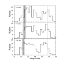
Figure 5: Luminosity functions for each of the narrow band filters. No correction for reddening or completeness has been made. The vertical dotted lines indicate the mean saturation and photometric completeness limits in each filter. Saturation occurs over a range in magnitude (grey bar) due to pixelization and variations in flat field reponse across the detector.

The luminosity functions (LFs) for each of the narrow band filters are shown in Fig. 5. No corrections for reddening or completeness have been made. The range in magnitude over which saturation occurs is indicated by the grey band in each panel. The vertical dotted lines indicate the mean saturation limit and the completeness limit of $17.5$ magnitudes. The F215N luminosity function is relatively flat between the saturation and completeness limits, with a dip between 14 and 15.5 magnitudes. The structure in the F166N and F190N luminosity functions is similar.

In order to compare our LF with previously determined LFs for IC348, we converted our measured F215N magnitudes to standard $K$ magnitudes. The F215N filter measures a relatively feature-free region of the standard CTIO/CIT $K$ filter. Therefore, the F215N magnitude should correlate well with $K$, requiring a zero-point offset and possibly, due to increasing water band strengths in the coolest M stars, a color term. To determine the offset, we compared our F215N magnitudes with published $K$ magnitudes for the 61 stars in our sample that are in common with Lada & Lada (1995; see tabulation in LRLL ) and/or Luhman (1999) and are below the saturation limit ($K>11$). The fit had a slope statistically identical to unity ($1.003\pm 0.012$), so we derived the mean offset between the two magnitude systems, $\langle(K-F215N)\rangle=-0.115\pm 0.011$, where the error is the error in the mean. The 1–$\sigma$ residual to the fit was $0.085$. This residual is comparable to the typical combined photometric accuracy of the Luhman and our data. We investigated a possible color term in the transformation, but found that if any is present it is smaller than this scatter about the mean.

The accuracy and completeness of the bright end of our luminosity function ($K\lesssim 11$) is compromised by both saturation and our deliberate avoidance of bright cluster stars. To correct for this deficiency, we combined our derived $K$ photometry at $K\geq 11$ with $K$ photometry of the $5\arcmin\times 5\arcmin$ core from LRLL for $K<11$. This combination is reasonable since, as shown in Fig. 1, the region of our survey largely overlaps the $5\arcmin\times 5\arcmin$ core. To correct for the different areas covered by two surveys, we multiplied the counts in each bin of the LRLL luminosity function by the ratio of the survey areas, $34.76/25.00=1.39$.

The combined $K$ luminosity function for our 34.76 sq. arcmin region, complete to $K\simeq 17.5$, is shown in Fig. 6 as the solid line histogram. To estimate the background contribution to the $K$ luminosity function, we used the prediction of the star count model of Cohen (1994). The predicted background $K$ counts, reddened by the mean reddening of the background population ($A_{K}=0.71$; see section 6), is shown as the dotted line histogram in Fig. 6. In section 8, we compare in greater detail the results for our data set with the predictions of the model. Here we simply note a few points. The contamination of the cluster by background stars is insignificant to $K\approx 13$ and the number of cluster stars is larger than the number of background stars until the $K=14.25$ bin. While the background rises steadily, we appear to have detected a few cluster stars to our completeness limit.

5 Spectral Classification

To derive spectral types for the stars in the sample, we combined the measured narrow band fluxes into a reddening independent index,

$$Q_{\rm H2O}\equiv-2.5\log{\left(\frac{\rm F166}{\rm F190}\right)}+1.37\times 2.5\log{\left(\frac{\rm F190}{\rm F215}\right)},$$

that measures the strength of the $1.9~{}\mu$m H₂O absorption band. In this expression, F166, F190, and F215 are the fluxes in the F166N, F190N, and F215N filters, respectively. The value 1.37 is the ratio of the reddening color excesses:

$$\frac{E({\rm F166/F190})}{E({\rm F190/F215})}=1.37,$$

which is derived from the infrared extinction law $A_{\lambda}/A_{V}=0.412(\lambda/\mu{\rm m})^{-1.75}$ (Tokunaga (1999)).

To explore the utility of the water index as an indicator of spectral type, we examined the relation between $Q_{\rm H2O}$ and spectral type for both the standard stars and a subset of IC348 stars that have optically determined spectral types from LRLL and Luhman (1999). For the standard stars, we adopted spectral types from the literature that are derived consistently from the classification scheme of Kirkpatrick et al. (1995). As shown in the top panel of Figure 7, $Q_{\rm H2O}$ is strongly correlated and varies rapidly with spectral type among the standard stars, confirming the expected sensitivity of the water band strength to stellar effective temperature. As is evident, there is real scatter among the standard stars that cannot be explained by errors in $Q_{\rm H2O}$ and spectral type. The scatter may reflect the inherent diversity in the standard star sample, a property that is evident from their $JHK$ colors. The spread in broad band color for a given spectral type is usually interpreted as the result of varying metallicity (e.g., Fig. 1 from Leggett et al. (1996)).

To compare these results with those for a population that has a more homogeneous metallicity distribution and the same mean metallicity and gravity to the IC348 sample, we also examined the $Q_{\rm H2O}$ vs. spectral type relation for the subset of IC348 stars that have optical spectral types determined by LRLL and Luhman (1999) (middle panel of Fig. 7). Although LRLL found no systematic difference between their IR and optical spectral types, there is significant dispersion between the two systems (their IR spectral types differ from the optical spectral types by as much as 3 subclasses). We find that the water band strengths are better correlated with the optical spectral types, with a smaller dispersion, than the IR spectral types, suggesting that their optical spectral types are more precise.

With the use of optical spectral types, we were also able to compare directly the results for the dwarf standards and the IC348 population, since both sets of objects are classified on the same system. The two samples exhibit a similar relation between spectral type and $Q_{\rm H2O}$ despite the difference in gravity between the two samples, with some evidence for a shallower slope for the pre-main sequence stars compared to the dwarfs. However, with the present data alone, we cannot claim such a difference with much certainty because the sample sizes are not large enough, the IC348 stars are not distributed evenly enough in spectral type, and there could be small systematic differences in the spectral typing of the IC348 and standard stars. The possibility of a difference between the two relations could be explored with more extensive optical spectral typing of the IC348 population.

The horizontal and vertical error bars in the lower left corner of the middle panel of Fig. 7 represent the typical errors in $Q_{\rm H2O}$ and spectral type for the cluster stars. Some of the scatter may arise from infrared excesses (which would uniquely affect the young star sample, compared to the standard star sample), although this effect is expected to be limited given the relatively small fraction of cluster sources that have IR excesses. For example, based on their $JHK$ photometry, Lada & Lada (1995) determined that $<$12% of sources brighter than $K=14$ in IC348a have substantial IR excesses. The LRLL study spectroscopically inferred $K$ continuum excesses in a similar fraction (15%) of sources in the subcluster.

To examine the possible impact of IR excess on our derived $Q_{\rm H2O}$ values, we considered excesses of the form $\Delta F_{\nu}(\lambda)\propto\lambda^{-\beta}$ and explored the effect of the excess on the $Q_{\rm H2O}$ values for two of our standards, the M3 dwarf Gl388, and the M6 dwarf Gl406. Since classical T Tauri stars have excesses at $K$ of $r_{K}\sim 0.6$ (Meyer et al. (1997); where $r_{K}$ is the ratio of the excess emission to the stellar flux), the IC348 sources, being more evolved, are likely to have much weaker excesses, typically $r_{K}<0.2$. With a spectral index of $\beta=1/3,$ appropriate for both disks undergoing active accretion and those experiencing passive reprocessing of stellar radiation, an IR excess produces an increase in $Q_{\rm H2O}$. Since the spectral slope is shallow and the maximum excess is small, only modest excursions are possible. For example, the $Q_{\rm H2O}$ index for Gl388 varies from its observed value, -0.28, at 0% excess to -0.24 at 20% excess in F215N. Over the same range of 0 to 20% excess in F215N, the $Q_{\rm H2O}$ index for Gl406 ranges from -0.52 to -0.43. This range of variation is sufficiently large that IR excess could account for most of the scatter of IC348 stars away from the mean trend to larger values of $Q_{\rm H2O}$. Explaining the scatter to smaller values of $Q_{\rm H2O}$ as the result of IR excesses requires more extreme values of $\beta$. For Gl388, values of $\beta<-3$ are needed to decrease $Q_{\rm H2O}$ from its value at 0% excess. Such extreme spectral indices are unlikely as they would produce unusual broad band colors. For these reasons, it appears unlikely that IR excess is responsible for the majority of scatter about the mean relation between $Q_{\rm H2O}$ and spectral type. Other processes are implied, possibly including those that produce true differences in stellar water band strengths among stars with equivalent $I$-band spectral types.

Since we were not able to distinguish a systematic difference between the mean trends for the standard star sample and the IC348 sample, we used the combined samples to calibrate the relation between $Q_{\rm H2O}$ and spectral type (lower panel of Fig. 7). In order to use the error information in both $Q_{\rm H2O}$ and spectral type, we performed a linear fit in both senses (i.e., spectral type vs. $Q_{\rm H2O}$ and $Q_{\rm H2O}$ vs. spectral type; dotted lines in Fig. 7) and used the bisector of the two fits as the calibration relation (solid line in Fig. 7). Due to the non-uniform distribution of stars along the fit, the slope of the fit is sensitive to the inclusion or exclusion of stars near the sigma-clipping limit and at the extremes of either $Q_{\rm H2O}$ or spectral type. Doing a fit in both senses, and including the error information in both quantities, allowed us to better identify and exclude outliers. In the lower panel of Fig. 7, solid symbols indicate the stars that were included in the fit while open symbols indicate excluded stars.

The equation of the bisector, the relation we subsequently used to estimate spectral class for the entire cluster sample, is:

$${\rm M~{}subtype}=-1.09(\pm 0.39)-13.01(\pm 0.50)\times Q_{\rm H2O}.$$ (5-1)

For a typical value of $Q_{\rm H2O}$, the formal spectral type uncertainty in the fit is $\pm 0.46$, while the scatter about the fit is $0.81$, just a little under one subtype. It is noteworthy that the discrete nature of spectral type versus the continuous nature of $Q_{\rm H2O}$ is responsible for a mean scatter of $0.77$ in $Q_{\rm H2O}$ in each subtype bin, which is a significant contribution to the total scatter.

Finally, we note that stars earlier than M2 have less certain spectral types due to the combination of the inherent scatter in the $Q_{\rm H2O}$ vs. spectral type relation and the decreasing sensitivity of the $1.9~{}\mu$m H₂O absorption band to spectral type as the K spectral types are approached. As a result, stars with spectral types of K and earlier can be misclassified by our method as later-type objects. For example, a comparison of the spectral types obtained by LRLL and Luhman (1999) with those obtained by our method shows that stars earlier than $\sim$K5 are classified by us as late K or M0 stars and late-K stars are classified as late-K and M0-M1 stars.

6 Extinction

Although the stellar spectral typing could be carried out without determining the reddening to each object, extinction corrections are required in order to investigate the masses and ages of cluster objects. We estimated the extinction toward each star by dereddening the observed F166/F190 and F190/F215 colors to a fiducial zero-reddening line in the color-color plane. Since extinction estimates for the dwarf standard stars were not available in the literature, we adopted the usual assumption that they suffer zero extinction. Figure 8 diagrams the process. First, we fit a line to the positions of the standard stars in the color-color plane (top panel), which is defined to be a locus of zero reddening. The WTTS were excluded from the fit. Gl569A was regarded as an outlier and also excluded from the fit. The resulting linear relation is:

$$-2.5\log{\left(\frac{\rm F166}{\rm F190}\right)}=-0.277(\pm 0.009)-0.358(\pm 0.083)\times-2.5\log{\left(\frac{\rm F190}{\rm F215}\right)}$$

with a mean deviation about the fit of 1–$\sigma=0.036$. The extinction toward each star in the cluster fields was determined from the shift in each color required to deredden the star to the zero-reddening line. The resulting extinction estimates and errors are given in column 11 of Table From Stars to Super-planets: the Low-Mass IMF in the Young Cluster IC348 . Note that the reddening vector (shown for $A_{V}=10$ in the bottom panel of Fig. 8), is nearly perpendicular to the standard star locus in the color-color plane. Consequently, reddening and spectral type are readily separable with moderate signal-to-noise photometry even given modest uncertainties in the slope of the reddening vector.

The subset of our standards used for the reddening calibration span the spectral class range K2V to M9V. This range is indicated by the dotted lines in the lower panel of Fig. 8. The few stars in the field with spectral types outside this range have extinction estimates based on the extrapolation of the fiducial line. As we show in Section 8, most of the early type stars are likely background objects. Finally, while the formal uncertainty in the fit of the fiducial line to the standards is small, 0.04 magnitudes, the scatter about the line for the latest standards is significantly larger than the scatter for the earlier standards (top panel of Fig. 8). Part of this scatter is due to the larger photometric errors; the late type standards are also the dimmest. However, four of the five late type standards fall above the fiducial line. In order from upper left to lower right these standards are LHS3003(M7V), Gl569B(M8.5V), VB10(M8V), LHS2924(M9V), and VB8(M7V). With the exception of VB8, these stars are aligned in the expected order in both colors but seem to be systematically shifted about 0.1 magnitudes to the red in $-2.5\log{({\rm F166/F190})}$. While we cannot exclude the possibility that the relationship is non-linear for dwarfs later than M6, some of the scatter about the fit may be due to inherent variation in the photometric properties of the standard stars.

We can compare our extinction estimates to those of LRLL for the M dwarfs common to both samples. In Figure 9, the horizontal error bars indicate the formal (1–$\sigma$) uncertainty in our $A_{K}$ estimate (typically $<0.1$ mag). LRLL used various extinction estimators, citing their internal errors rather than values for individual stars. Their errors in $A_{K}$ range from 0.07 to 0.19 mag for the stars shown with a nearly equal systematic uncertainty in the zero point. For the M-dwarfs common to both samples, the mean difference in $A_{K}$, in the sense $\langle{\rm Ours-LRLL}\rangle=-0.01\pm 0.03$ with a scatter about the mean of 0.24 magnitudes. Considering the uncertainties, the agreement is good.

The resulting $A_{K}$ distribution (Fig. 10; solid-line histogram), has a pronounced tail to large values of $A_{K}$ and a peak at $A_{K}=0.1$. The extinction distribution for the subset of objects identified as the background population (as determined in section 8; dashed-line histogram) is also shown. Note that our extinction estimates include a few negative values (Figs. 8 and 9). While these values might suggest that our fiducial line needs to be lowered to bluer colors, that would imply a bias toward larger extinctions given the distribution of standard stars in the color-color plane. Therefore, we retain our original fit and, for all subsequent analysis, stars with negative extinction estimates are assigned an extinction of 0.0 with an error equal to the greater of the absolute value of the original extinction estimate or the formal uncertainty in the estimate.

With this revision, the mean extinction is $\langle A_{K}\rangle=0.44$ with an error in the mean of 0.04 and a median of $(A_{K})_{\frac{1}{2}}=0.31$. Our adjustment of the negative values impacts negligibly on the statistics. (If the negative extinction values were retained, the mean would be $\langle A_{K}\rangle=0.43$ with the error and median unchanged.) When our sample is restricted to those stars in common with LRLL , we find approximately the same mean reddening ($\langle A_{K}\rangle=0.30$) that they quote for their sample ($\langle A_{K}\rangle=0.34$). The larger mean reddening in the present study indicates that, on average, we have sampled a more extincted population of the cluster than has been investigated previously. Using the position of the main sequence at the distance of the cluster (see section 8) to divide the sample into cluster and background objects, we find that the cluster objects have $\langle A_{K}\rangle=0.31\pm 0.04$ with a scatter about the mean of 0.36. The background stars, which include most of the stars in the extended high extinction tail, have $\langle A_{K}\rangle=0.71\pm 0.07$, with a scatter about the mean of 0.49.

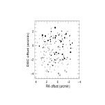
Figure 11: The spatial distribution of extinction and sample membership for all of the stars in our sample. The point size is scaled to the estimated extinction to each object (larger points corresponding to larger reddening), which ranges from $A_{K}=0.00$ to 2.33. The gray points represent objects in common with previous studies (LRLL ; Herbig (1998); Luhman (1999); see Table From Stars to Super-planets: the Low-Mass IMF in the Young Cluster IC348 ). The black points represent objects without previous reddening estimates.

The more heavily reddened stars in our sample are spatially intermixed with stars experiencing lower extinction. Figure 11 shows the same area plotted in Fig. 1. The gray symbols denote stars in our sample that were observed by other investigators (LRLL ; Herbig (1998); Luhman 1999), whereas the black symbols denote stars that were not observed by these investigators. The point size is scaled to our estimate of the extinction to the object (larger points corresponding to larger reddening), which ranges from $A_{K}=0.0$ to $A_{K}=2.33$. The higher average extinction among the black points is apparent. The extinction distribution is characterized by an overall gradient from NE (larger values) to SW (smaller) with significant small scale variation. Given the broad extinction distributions for both cluster and background objects, and the patchy distribution of extinction on the sky, it is evident that cluster membership cannot be determined on the basis of extinction alone. Membership based on extinction would erroneously assign low extinction background members to the cluster and highly extincted cluster members to the background.

7 Observational HR Diagram

With the spectral types determined in section 5 and the extinction extimates from section 6, we can construct an observational HR diagram of the cluster fields. In Figure 12, the vertical axes are apparent $K$ magnitude (left panel) and dereddened $K$ magnitude, $K_{0}$ (right panel). For comparison, the solid curve in the right panel is the fiducial main sequence at the distance of the cluster (see section 8.2). Examination of both panels reveals a well defined cluster sequence at $K\leq 14$. This locus is marginally tighter after being dereddened which supports the accuracy of our reddening estimates.

Spectral type errors are not shown, both to limit confusion and because some stars have systematic as well as random error. For example, although the typical random error is $\pm 1$ spectral subtype, stars earlier than M2 have systematically later $Q_{\rm H2O}$ spectral types than optical spectral types (section 5). Given the possible inaccuracy of our spectral typing scheme at spectral types earlier than M2, we adopted the optical spectral types of Luhman (1999) or LRLL for these objects where available. The original $Q_{\rm H2O}$ spectral types of these stars are shown as open circles in Figure 12. When optical spectral types of these stars are adopted instead (see subsequent figures), the photometric width of the distribution at M2 and earlier is reduced. In general, the random error in spectral type increases with increasing magnitude (see column 13 of Table From Stars to Super-planets: the Low-Mass IMF in the Young Cluster IC348 ). All stars with $K<15.5$ have spectral type errors $\leq 1$ subtype. Since our spectral type errors grow rapidly below $K=16$, with stars fainter than $K=16.5$ having spectral type errors $\gtrsim 2.5$ subtypes, we identify $K=16.5$ as our effective magnitude limit for accurate spectral typing.

While some objects have spectral types as late as “M13”, this should be interpreted simply as an indication of strong water absorption rather than an advocacy of M spectral types beyond M9. The existence of objects with stronger water absorption than that of M9 dwarfs is in general agreement with the predictions of atmospheric models (e.g., the Ames-Dusty and Ames-MT-Dusty models of Allard et al. (2000)). These suggest that even in the presence of dust, the $1.9~{}\mu$m H₂O absorption band continues to increase in strength down to $\sim 2000$ K at pre-main sequence gravities. In the Ames-Dusty models, $Q_{\rm H2O}$ increases in strength by 45% between 2450K (equivalent to M8 in the dwarf temperature scale; see section 8.2) and 2000K. The $Q_{\rm H2O}$ vs. spectral type relation in eq. 5-1 implies that $Q_{\rm H2O}$ is 54% stronger at M13 than at M8, in general agreement with the predictions.

The dearth of stars at $K\approx 15.5$ in the $K$ luminosity function is also evident in the left panel of Fig. 12. Part of the deficit is due to the higher average reddening of the background stars. Stars with $K>15.5$ have an average extinction greater than stars with $K<15.5$ and when they are dereddened, they fill in the deficit somewhat. Our photometric completeness limit of $K=17.5$ is shown in the left panel as a horizontal dotted line. To quantify our detection limit as a function of extinction, we also show the completeness limit dereddened by $A_{K}=0.31$, the mean extinction among the cluster stars (lower horizontal dotted line in the right panel of Fig. 12) and by $A_{K}=2.33$, the greatest extinction detected in the cluster fields (upper horizontal dotted line). Both limits, $K=17.19$ and $K=15.17$, are considerably dimmer than the typical cluster M star.

These results imply that we have fully sampled the cluster population over a significant range in extinction. The extinction range that we probe is, of course, a function of spectral type. As examples, of the two cluster stars in the tail of the reddening distribution shown in Fig. 10, one is an M2 star with $K=12.16$ ($A_{K}=1.97$) and the other is an M9 star with $K=16.73$ ($A_{K}=1.52$). We would have been able to detect and spectral type the first star through another $\sim 4.4$ mag of extinction (to $A_{K}\approx 6.4$). The second star, observed through almost 5 times the average cluster extinction, is close to our spectral typing limit.

8 Comparison with Evolutionary Tracks

8.1 Evolutionary Models

Evolutionary models for low mass objects have developed greatly in recent years, with several different models now available over a large range in mass. D’Antona & Mazzitelli (1997) have recently updated their pre-main sequence calculations, retaining the use of the Full Spectrum Turbulence model of Canuto & Mazzitelli (1991) and making improvements in opacities and the equation of state. For the purpose of this paper, we use their 1998 models (hereinafter DM98) which cover the mass range $0.017-0.3M_{\odot}$ and include further improvements, e.g., in the treatment of deuterium burning, that affect the very low mass tracks.

Other groups (e.g., Baraffe et al. (1998); Burrows et al. 1997) have also presented new evolutionary models that include improvements in the treatment of the stellar interior and use non-gray atmospheres as an outer boundary condition. The corrections associated with the latter are particularly significant at low masses since the presence of molecules in low temperature atmospheres results in spectra that are significantly non-blackbody. Models by Baraffe et al. (1998; hereinafter B98) explore the mass range $\sim 0.025-1.0M_{\odot}$ using the Allard et al. (1997) NextGen synthetic atmospheres. Although there are known inconsistencies in the NextGen models (e.g., they overpredict the strength of the IR water bands; TiO opacities are suspected to be incomplete; grain formation is not included), the B98 models nevertheless reproduce well the main sequence properties of low metallicity populations, e.g., the optical color-magnitude diagram of globular clusters and halo field subdwarfs. There is also good agreement with the optical and IR properties of nearby disk populations, although some discrepancies remain at low masses ($<0.15M_{\odot}$).

Non-gray models have been developed independently by Burrows et al. (1997) who focus on the properties of objects at lower mass ($0.3-70M_{J}$, where $M_{J}$ is the mass of Jupiter). The Burrows et al. evolutionary tracks differ qualitatively from those of B98 in the upper mass range, but are more qualititatively similar at masses $\lesssim 60M_{J}.$ The qualitative difference between these models, which appear to have similar input physics, may indicate the current level of uncertainty in the evolutionary tracks at low masses. Quantitatively, an effective temperature of 3340 K and luminosity of $0.076L_{\odot}$ corresponds to a mass and age of $0.090M_{\odot}$ and 1.8 Myr with the Burrows et al. tracks and $0.3M_{\odot}$ and 8 Myr with the B98 tracks. The tracks agree better in mass in the lower mass range: at 2890 K and $0.022L_{\odot}$, Burrows et al. predict $0.05M_{\odot}$ at 1.2 Myr, and the B98 tracks predict $0.06M_{\odot}$ at 3.2 Myr.

8.2 Interloper Population

As reviewed by Herbig (1998), the distance to IC348 has been previously estimated on the basis of both nearby stars in the Per OB2 association and stars in the IC348 cluster itself. For the purpose of comparing our results with evolutionary tracks, we adopt a distance to IC348 of $d=300$ pc, $(m-M)_{0}=7.4$. This value is in good agreement with current estimates of the distances to the Per OB2 cluster (318$\pm 27$ pc; de Zeeuw et al. 1999) and to IC348 itself (261$\pm 25$ pc; Scholz et al. 1999) inferred from Hipparcos data. The adopted distance is also in agreement with the value adopted by both Herbig (1998) and LRLL and thereby allows ready comparison of our results with those obtained in previous studies.

To delineate the background population, the position of the main sequence at the cluster distance is indicated by the solid curve in the right panel of Fig. 12, where we have used the 12 Gyr isochrone from the B98 evolutionary tracks and a temperature scale that places the isochrone in good agreement with the main sequence locus of nearby field stars (e.g., Kirkpatrick & McCarthy (1994)). The temperature scale used,

$${\rm M~{}subtype}=(4000-T_{\rm eff})/180,$$

is generally consistent with the Leggett et al. (1996) dwarf temperature scale.

The magnitude and spectral type distributions of the background population, located to the lower left of the main sequence, are in very good agreement with the total interloper population predicted by models of the point source infrared sky (Wainscoat et al. (1992); Cohen 1994) at the Galactic latitude and longitude of IC348. Table 4 compares the observed and model counts as a function of $K$ magnitude and spectral type. To $K_{0}=17$, significant departures between the model and observed counts are apparent only for spectral types earlier than M3 at $K_{0}>16$. Given the large spread in the reddening distribution of the background population (to $A_{K}>2$; Fig. 10), this discrepancy in the counts probably arises from photometric incompleteness below $K=17.5$. This result (the good agreement between the model prediction for the total interloper population and the observed background population), implies a negligible foreground contamination (at most $1-2$ stars) of the cluster population at late spectral types. The large reddening of many of the faint late-type stars also statistically argues against a foreground origin for these objects. Note, however, that the errors on some of the fainter objects identified as older cluster members (e.g., objects in the range $K_{0}=15.5-16.5$, M6$-$M8) allow for the possibility that they are background objects even if they are not predicted to be so by the Galactic structure model.

8.3 Temperature Scale and Bolometric Correction

A generic difficulty in comparing measured stellar fluxes and spectral types with evolutionary tracks is the need to adopt relations between spectral type, effective temperature, and bolometric correction. In principle, such relations could be avoided by using synthetic spectra from model atmospheres to go directly from observed spectra and colors to temperature and gravity, and hence to mass and age using the theoretical evolutionary tracks. For example, we might hope to compare directly the water band strengths of the Allard & Hauschildt atmospheres used in the B98 models with the water band strengths that we measured. However, since there remain significant quantitative differences between the predicted and observed water band strengths of M stars (e.g., the models consistently overpredict water band strengths; see also Tiede et al. (2000)), this approach cannot be used in the present case. In other words, although current synthetic atmospheres may be sufficiently accurate for the purpose of evolutionary calculations and the prediction of broad band colors, they are insufficiently accurate as templates for spectral typing. Hence, we adopted the less direct method of first calibrating our water index versus spectra type (section 5), and then selecting an appropriate spectral type to temperature conversion.

Ideally, we would want to use a relation between spectral type and effective temperature that is appropriate to the gravity and metallicity of the IC348 population. Unfortunately, an empirical calibration of spectral type and effective temperature appropriate for pre-main-sequence conditions has yet to be made. In the meantime, since pre-main-sequence gravities are similar to dwarf gravities, temperature scales close to the dwarf scale (e.g., Leggett et al. (1996)) are often used in the study of young populations (e.g., LRLL; Wilking et al. (1999)). Because the temperature scale may differ from that of dwarfs at PMS gravities, other choices have also been investigated, including temperature scales intermediate between those of dwarfs and giants (e.g., White et al. (1999); Luhman 1999).

The validity of the various evolutionary tracks can be evaluated by a number of criteria including whether stellar masses predicted by evolutionary tracks agree with dynamical estimates, and whether populations believed to be coeval appear so when compared with evolutionary tracks (e.g., Stauffer et al. 1995). Dynamical mass constraints are becoming available in the $1M_{\odot}$ range (see, e.g., Mathieu et al. (2000)) but are thus far unavailable at the masses of interest in the present study. In contrast, coeval population constraints are more readily available at these lower masses. For example, in the GG Tau hierarchical quadruple system (White et al. (1999)), the four components of the system, arguably coeval, span a wide range in spectral type (K7 to M7; open squares in Fig. 13, upper left), thereby outlining, in rough form, an isochrone spanning a large mass range. When plotted at a common distance, the IC348 cluster locus identified in the present study overlaps the locus defined by the GG Tau components over the same range of spectral types (Fig. 13). This both reinforces the validity of the GG Tau system as a coeval population constraint and argues that the mean age of the IC348 cluster is approximately independent of mass. Similar results have been found previously at spectral types earlier than M6 (Luhman 1999).

The uncertainty in the pre-main-sequence temperature scale complicates our understanding of the validity of the tracks. As discussed by Luhman (1999), combinations of evolutionary tracks and temperature scales that are consistent with a coeval nature for the GG Tau system and the IC348 cluster locus include (1) DM98 tracks and a dwarf temperature scale (2) B98 tracks and an otherwise arbitrary temperature scale intermediate between that of dwarfs and giants. Our results are compared in Figure 13 with these combinations of temperature scales and tracks. For comparison, the two alternative combinations of temperature scales and tracks are shown. In comparing the B98 models with the observations, we have used the model $K$ magnitudes and a linear fit to either the dwarf temperature scale

$${\rm M\ subtype}=(3914-T_{\rm eff})/183.3$$ (8-1)

or the Luhman (1999) intermediate temperature scale

$${\rm M\ subtype}=(3850-T_{\rm eff})/141.0$$ (8-2)

In approximating the dwarf temperature scale, particular weight was given to the dwarf temperature determinations by Tsuji et al. (1996) who used the IR flux measurement technique. As they show, this technique is relatively insensitive to the details of synthetic atmospheres (e.g., dust formation). The fit thus obtained is in good agreement with the temperature determinations of Leggett et al. (1996) which are based on a comparison of synthetic atmospheres with measured IR colors and spectra. In comparing the DM98 models with the observations, we have used, in addition to these temperature scales, a bolometric correction

$${\rm BC_{K}}=M_{\rm bol}-M_{K}=4.19-T_{\rm eff}/2240$$

that extrapolates the values obtained by Leggett et al. (1996) and Tinney et al. (1993) to low temperatures.

The combination of the B98 models and the Luhman intermediate temperature scale (eq. 8-2; Fig. 13 upper left) implies that the mean age of the cluster is approximately independent of mass over the range $0.7-0.04M_{\odot}$. The comparison implies a mean age $\sim$3 Myr with a age spread from $<1$ to $\sim 20$ Myr. The faint cluster population between spectral types M5 and M8 appears to constitute an old cluster population ($\sim 5$ to $>20$ Myr) with masses $0.13-0.05M_{\odot}$. If the dwarf temperature scale (eq. 8-1; Fig. 13 upper right) is used instead, the cluster is, on average, significantly younger at late spectral types.

The combination of the DM98 models and the dwarf temperature scale (eq. 8-1; Fig. 13 lower right) implies that the mean cluster age is approximately independent of mass at spectral types earlier than M7 but younger at late types. The comparison implies a mean age $\sim 1$ Myr with a age spread from $<1$ to $\sim 10$ Myr. With these models, the faint cluster population between spectral types M5 and M8 is spread over a larger range in mass $0.16-0.025M_{\odot}$. If the Luhman intermediate temperature scale (eq. 8-2; Fig. 13 lower left) is used instead, the cluster is older at late types with a larger spread in age. With all combinations of models and temperature scales, the brighter cluster population beyond M8 is systematically younger, $<1$ Myr old. If this is an artifact, it may indicate the likely inadequacy of the assumed linear relation between effective temperature and spectral type over the entire range of spectral types in the sample. Deficiencies in the evolutionary tracks are another possibility.

It is interesting to examine the motivation for the intermediate temperature scale adopted by White et al. (1999) and Luhman (1999). These authors have argued that since the M giant temperature scale is warmer than the dwarf scale, PMS stars, which are intermediate in gravity, may be characterized by a temperature scale intermediate between that of giants and dwarfs. Luhman (1999) has further shown that the spectra of pre-main sequence stars in IC348 are better fit by an average of dwarf and giant spectra of the same spectral type.

There are several caveats to this argument. Firstly, the giant temperature scale considered by Luhman (1999) is derived from the direct measurement of stellar angular diameters (e.g., Perrin et al. (1998); Richichi et al. (1998); van Belle et al. 1999 ), whereas the dwarf temperature scale is typically determined with the use of model spectra (e.g., Leggett et al. (1996); Jones et al. (1994); Jones et al. (1996)). The different methods by which the two temperature scales are derived may introduce systematic differences that do not reflect a true temperature difference.

Secondly, we can turn to synthetic atmospheres for insight into the gravity-dependent behavior of the temperature scale. In the current generation of the Allard & Hauschildt atmospheres (e.g., Ames-Dusty, Ames-MT-Dusty), the 1.9$\mu$m water band strength is relatively insensitive to gravity above 3000K ($\sim$M5 in the dwarf scale). At effective temperatures below 3000K, dust formation is significant, introducing added complexity to the gravity dependence of the atmosphere in the 1.9$\mu$m region. In this temperature range, the water index first increases in strength ($Q_{\rm H2O}$ decreases) at fixed temperature from $\log g\sim 3.5$ to $\log g\sim 5.0-5.5$ (due to increased water abundance) then decreases in strength with higher gravity (due to increased dust formation and consequent backwarming and dissociation of water). The net result is a cooler temperature scale for pre-main-sequence gravities below 3000K. For example, at $\sim 2700$ K pre-main-sequence objects ($\log g=3.5-4.0$) are $\sim 200$K cooler than dwarfs ($\log g=5.0-5.5$) with an equivalent water strength.

On the basis of these models, there is little physical motivation for an intermediate temperature scale beyond M4 for the interpretation of water band strengths. Of course, these considerations apply to the interpretation of 1.9$\mu$m water band strengths rather than the 6500-9000Å region studied by Luhman (1999). A detailed examination of current synthetic atmospheres for the latter spectral region may provide better motivation for a hotter temperature scale at lower gravities.

Note that the gravity dependence of $Q_{\rm H2O}$ in the synthetic atmospheres is modest over the range of gravities relevant to low mass pre-main sequence stars in the age range of the cluster (1–10 Myr). For example, in the B98 model, an $0.06M_{\odot}$ object follows a vertical evolutionary track at $T_{\rm eff}\sim 2860$K with $\log g=3.6-4.2$ in the age interval 1–10 Myr which corresponds to a fractional change in $Q_{\rm H2O}$ of $\lesssim 15$% or $\lesssim 1$ subtype, given the relation between $Q_{\rm H2O}$ and spectral type discussed in section 5.

In summary, while we can find little physical motivation for an intermediate temperature scale with which to interpret our results, we interpret the better fit to the IC348 cluster locus that we obtain with the combination of this temperature scale and the B98 models as an indication of the direction in which the evolutionary model calculations might themselves evolve in order to better reproduce observations of young clusters. With these caveats in mind, we discuss, in the next section, the cluster mass function implied by 2 combinations of tracks and temperature scales. However, it is already clear that there will be reasonable uncertainty associated with such results.

9 Discussion

9.1 Binarity

The area and depth that we have covered at relatively high angular resolution, combined with our ability to discriminate cluster members from background objects, allows us to place some useful constraints on the binary star population of the cluster. At the pixel scale of NIC3, pairs of stars with separations $\gtrsim 0.8\arcsec$ are easily identified over the entire magnitude range of our sample; for fainter primaries, companions could be similarly detected at smaller separations. A significant obstacle to the detection of faint companions at separations $\lesssim 0.8\arcsec$ is the complex, extended structure in the NICMOS PSF which also makes it difficult to quantify our detection completeness. More refined techniques, such as PSF subtraction or deconvolution, when applied to the data, are likely to reveal close binary systems that we have missed.

Table 5 tabulates all of the stars in our sample that were found to have a nearest neighbor within $8\arcsec$. The stars have been designated primary and secondary based on their $K_{0}$ magnitudes. The spectral types for the G dwarfs are from LRLL and the other spectral types are our spectral types as determined in Section 5. Figure 14 shows the positions of the close pairs in the observational HR diagram. To identify the pairs, the components are connected by lines. Although we were sensitive to separations $\gtrsim 0.8\arcsec$, only pairs with separations $>1.5\arcsec$ were detected. Based on their locations in the observational HR diagram, seven of the close pairs are chance projections of a background star close to a cluster member (Fig. 14; dotted lines). Both components of one pair are background objects. Of the 8 candidate cluster binaries 3 (093-04/093-05; 043-02/043-03; 024-05/024-06) were previously detected by Duchene et al. (1999) in their study of binarity among a sample of 67 IC348 objects. We also confirm their speculation that 083-03 and 023-03 are background objects with small projected separations to cluster members.

As shown in Fig. 14 (solid lines), several of the candidate binary pairs have spectral types and $K_{0}$ magnitudes consistent with a common age for the two components. For the candidate binaries E, F, C, D, and H, the lines connecting the two components have slopes consistent with the isochrones. The candidate binary B has a nearly vertical slope. However, given our estimate of the uncertainty in the spectral types of the binary components, the slope is also highly uncertain, and a common age for the binary components cannot be ruled out. While the component spectral types for the binary candidate G have similar uncertainties, the large separation in magnitude between the two components, if each are single stars, makes it unlikely that they share a common age. If, on the other hand, the brighter component is an approximate equal mass binary, the reduced brightness of each of the two stars is more consistent with the evolutionary models, and the triple system may be coeval. If more definitive studies reveal that the binary candidates B and G are not coeval, this may indicate that they are not physically related. Alternatively, a large age difference between the components may indicate that the binaries formed through capture.

If we define the binary fraction as the ratio of the number of companions detected to the number of targets observed (193 stars), the cluster binary fraction in the separation range $0.8\arcsec-8\arcsec$ (240 $-$ 2400 AU) is 8%. This is comparable to the result of Duchene et al. (1999) who, based on a smaller sample of stars, found a 19% binary fraction for their entire sample; half of their binaries fall in the separation range of our study. However, there are several important differences between the two studies. We sample a lower range of primary masses ($\sim 0.015-0.8M_{\odot}$) than Duchene et al. (1999) ($\sim 0.2-2M_{\odot}$). In addition, the mass ratios to which we are sensitive are set by the magnitude limit of the sample rather than by the magnitude difference between the binary components. In contrast to Duchene et al. (1999), who commented on the lack of substellar companions, we find candidate substellar companions (e.g., 022-05) and one candidate substellar binary (H).

9.2 Low-Mass Cluster Members

The very low-mass cluster population is highlighted in Figure 15. The 6 objects indicated have the largest water absorption strengths in the sample, corresponding to spectral types later than M9, and presumably the lowest masses. The errors on the derived properties for 3 of the objects (012-02, 102-01, 022-09) are modest, and imply masses $\lesssim 0.025M_{\odot}$ in the context of both the B98 and DM98 models. The other 3 objects (024-02, 075-01, and 021-05) are in fact fainter than our effective limit for accurate spectral typing ($K=16.5$) and so have spectral type errors $>2.5$ subtypes (cf. section 7). Two of these objects, 024-02 ($A_{K}=1.52$) and 075-01 ($A_{K}=2.3$), are faint due to their large extinctions and are $\sim 5$ and $\sim 7$ times more extincted, respectively, than the cluster mean. Even with the larger errors for these objects, it appears very likely that all 3 are substellar cluster objects. However, because of its proximity to the main sequence, there is a small probability that 021-05 is a background M star.

9.3 Mass Function

To estimate a mass function for our sample, we used two combinations of evolutionary models and temperature scales: the B98 models in combination with the Luhman (1999) intermediate temperature scale and the DM98 models in combination with the dwarf temperature scale. The lower mass limit to which we are complete is determined by our spectral typing limit. As discussed in section 7, we have fairly accurate spectral types for all sources to $K=16.5$. For a mean cluster reddening of $A_{K}\simeq 0.3,$ this corresponds to $K_{0}\simeq 16.2$ or $M_{K}\simeq 8.8$ at the assumed distance of IC348. Thus, with the DM98 models, we are, for example, complete to $0.017M_{\odot}$ at the mean extinction of the cluster and ages $<3$ Myr.

For the B98 models, some extrapolation was needed to both younger ages ($<2$ Myr), in order to account for the brighter cluster population, and to lower masses ($<0.025M_{\odot}$) in order to estimate our mass completeness limit. In extrapolating below 2 Myr, we used the 1 Myr isochrone from the Baraffe et al. (1997) models as a guide. For the lower masses, we used the planetary/brown dwarf evolutionary theory of Burrows et al. (1997) to extrapolate the isochrone appropriate to the mean age of the subcluster (3 Myr). Several similarities between the Burrows et al. and B98 models suggest the utility of such an approach. Like B98, the Burrows et al. theory is non-gray, and the evolutionary tracks in the luminosity vs. $T_{\rm eff}$ plane at masses $<0.04M_{\odot}$ are qualitatively similar. Two possible extrapolations are given to illustrate the uncertainty in the result.

In the B98 models, a $0.025M_{\odot}$ object at 3 Myr has $T_{\rm eff}=2628$K, and $M_{K}=7.56$. In comparison, in the Burrows et al. theory, a $0.025M_{\odot}$ object at 3 Myr is slightly hotter ($T_{\rm eff}$=2735K) but has a comparable absolute $K$ magnitude ($M_{K}=7.6$ assuming BC${}_{K}=3.0$); a 3 Myr old object that is 1.2 magnitudes fainter ($M_{K}=8.8$) has an effective temperature $\simeq 300$K cooler and is $0.011M_{\odot}$ lower in mass. Applying the same mass and temperature differentials to the 3 Myr old, $0.025M_{\odot}$ object from B98 implies that a 3 Myr old, $M_{K}=8.8$ object in the B98 theory has $T_{\rm eff}=2330$K and a mass of $0.014M_{\odot}$.

As an alternate estimate, we can extrapolate the 3 Myr isochrone based on a match in $T_{\rm eff}$ rather than mass. As described above, the effective temperature of a $0.025M_{\odot}$, 3 Myr old object in B98 theory is 2628K. From the $T_{\rm eff}=2628$K point in the 3 Myr isochrone of the Burrows et al. models, $\Delta M_{K}=1.2$ corresponds to a change in temperature and mass of $\Delta T_{\rm eff}=-425$K and $\Delta m=-0.010M_{\odot}$. Applying these mass and temperature differentials to the 3 Myr old, $0.025M_{\odot}$ object from B98 implies an effective temperature of $2200$K and mass $0.015M_{\odot}$ for a 3 Myr old, $M_{K}=8.8$ object. Thus, with either estimate, our spectral typing limit of $M_{K}=8.8$ corresponds to a mass completeness limit of $\sim 0.015M_{\odot}$ at the average age and reddening of the cluster members. The effective temperature appropriate to this mass limit is less certain.

Formally, the appropriate effective temperature affects our estimate of the lower limit to the final mass bin of our sample. Note, however, that our spectral typing limit of $0.015M_{\odot}$ is close to the deuterium burning limit (Burrows et al. 1993, Saumon et al. 1996) and in the age range in which objects fade fairly rapidly with age. For example, in the Burrows et al. models, a 3 Myr old, $0.010M_{\odot}$ object is half as luminous as a $0.015M_{\odot}$ object at the same age. Given the rapid fading, it is unlikely that we have detected objects much less massive than $0.015M_{\odot}$, which we adopt as the lower limit of the final mass bin of the sample. Note that our spectral typing limit of $K=16.5$ implies that we have somewhat underestimated the population of the final mass bin if that bin is characterized by the same spread in age and reddening that is measured at higher masses.

The mass functions for the age range $0-10$ Myr that result from the assumptions and extrapolations discussed above are shown in Fig. 16. The result for both the B98 models (solid symbols) and DM98 models (dotted symbols) are shown. Note that the objects indicated previously as potential background objects ($K_{0}=15.5-16.5$, M6$-$M8) are not included in the mass function for the B98 models, whereas some are included in the mass function for the DM models. Since these objects represent only a small fraction of the objects in each bin, whether or not these are included as members makes little difference to the slope of the mass function.

The DM98 models indicate a flattening at $\sim 0.25M_{\odot},$ whereas the B98 models imply an approximately constant slope over the entire mass range $0.7-0.015M_{\odot}.$ In either case, the mass function appears to decrease from $\sim 0.25M_{\odot}$, through the hydrogen burning limit ($\sim 0.08M_{\odot}$), down to the deuterium burning limit ($\sim 0.015M_{\odot}$). The slope of the mass function in this range is consistent with $dN/d\log M\propto M^{0.5}$ for B98 and $dN/d\log M\propto M^{0.6}$ for DM98. The slow, approximately continuous decrease in the mass function in this interval differs from the result obtained by Hillenbrand (1997) for the Orion Nebula Cluster. The sharp fall off in the Orion Nebula Cluster mass function below $\sim 0.2M_{\odot}$ ($dN/d\log M\propto M^{2.5}$) is not reproduced here. Instead, we find that the slope of the IC348 mass function is more similar to that derived for the Pleiades in the mass range $0.3-0.04M_{\odot},$ $dN/d\log M\propto M^{0.4}$ (Bouvier et al. (1998)). The slope is similar to that inferred for the substellar population of the solar neighborhood from 2MASS and DENIS data. As determined by Reid et al. (1999), the observed properties of the local L dwarf population are consistent with a mass function $dN/d\log M\propto M^{\alpha},$ with $\alpha\sim$ -1 to 0, although a mass function similar to that for IC348 is not strongly precluded especially given the uncertainty in the age distribution of objects in the solar neighborhood.

Given the low masses to which we are sensitive, it is also interesting to compare our result to the mass function that is emerging for companions to nearby solar-type (G$-$KV) stars at separations $<5$ AU (e.g., Marcy et al. (2000)). While initial results indicated that the substellar companion mass function might be a smooth continuation of the stellar companion mass function (e.g., $dN/d\log M\propto M^{0.6}$; Mayor et al. (1998)), proper motion data from Hipparcos have revealed that a significant fraction of companions in the $0.015-0.08M_{\odot}$ range are low inclination systems, and hence have larger (stellar or near-stellar) masses (Marcy et al. (2000); Halbwachs et al. 2000). When corrected for these low inclination systems, the companion mass function appears to be characterized by a marked deficit in the $0.015-0.08M_{\odot}$ mass range (the “brown dwarf desert”; Marcy et al. (2000); Halbwachs et al. 2000). In contrast, the mass function for IC348 appears to decrease continuously through the stellar/substellar boundary and the mass range $0.08-0.015M_{\odot}$.

The low mass end of the IC348 sample extends into the mass range ($10-20M_{J}$) in which objects transition from higher mass objects that burn deuterium early in their evolution to lower mass objects that are incapable of deuterium burning due to the onset of electron degeneracy pressure during the contraction phase (e.g., Grossman et al. (1974); Burrows et al. (1993)). According to the calculations of Saumon et al. (1996), $\sim 15M_{J}$ objects deplete their deuterium abundances by a factor of 2 after 30 Myr of evolution, while objects $\leq 12M_{J}$ retain all of their initial deuterium and derive no luminosity from thermonuclear fusion at any point in their evolution. They suggest the deuterium burning limit as a possible interpretive boundary between objects that are regarded as brown dwarfs and those regarded as planets.

If we assume that the hydrogen and deuterium burning mass limits delimit the brown dwarf population, with either the DM98 or B98 models, we have fully sampled the brown dwarf population, at ages up to the mean age of the subcluster and extinctions up to the cluster average. Thus, we can conclude with near certainty that the fraction of the subcluster mass contributed by brown dwarfs is low, only a few percent of the cluster mass. With the B98 tracks, we find a total of $\sim 22$ cluster substellar candidates which represents a significant fraction, $\sim 20$%, of all cluster M dwarfs by number, but only a small fraction, $\sim 4$%, by mass. For comparison, with the DM98 tracks, we find $\sim 30$ cluster substellar candidates which represents $\sim 30$% of all cluster M dwarfs by number and $\sim 6$% by mass.

These limits on the substellar contribution to the total cluster mass have interesting implications when compared with current limits placed by microlensing studies on the substellar content of the Galactic halo. Based on the search for microlensing toward the LMC the current EROS limits on the fraction of the halo mass that resides in brown dwarf mass objects is $\lesssim$ 10% (Lasserre et al. 2000). Scaling our results for IC348 by the stellar fraction of the halo mass ($\sim 1$ %), we find that if the halo has the same IMF as IC348, then substellar objects contribute negligibly to the halo mass ($<0.1$%). The several orders of magnitude difference between these limits leaves room for some interesting possibilities. If future microlensing results find confirmation for a halo mass fraction of even $\sim 1$ % in substellar objects, that would indicate that low mass star formation in the halo proceeded significantly differently from that currently occuring in Galactic clusters.

What do the IC348 results tell us about the star formation process? The absence of structure in the mass function at the hydrogen burning limit (e.g., a turnover) is perhaps expected. It is difficult to imagine how hydrogen burning, which demarcates the end of the pre-main sequence phase, could influence the determination of stellar masses, an outcome which is probably determined at much earlier times.

We also find no obvious feature in the IMF at the deuterium burning limit (e.g., a strong increase or decrease), a potentially more relevant mass scale for star formation since deuterium burning occurs at pre-main-sequence ages. This result may appear puzzling in the context of some current theories for the origin of stellar masses. For example, in a canonical theory of the formation of solar-type stars, it is the onset of deuterium burning that is believed to set in motion the sequence of events by which a star comes to have a role in determining its own mass. The onset of deuterium burning first induces a fully convective stellar interior. The convective interior, combined with the rapid stellar rotation that is likely to result from the accretion of angular momentum along with mass, is believed to generate a strong stellar magnetic field. The strong field is, in turn, believed to drive a magnetocentrifugal wind that ultimately sweeps away the cloud from which the star formed and possibly reverses the infall itself, thereby helping to limit the mass of the star. The self-deterministic aspect of such a mass-limiting wind is a critical element in explanations for the generic origin of stellar masses (e.g., Shu (1995)) and some theories of the IMF (e.g., Adams & Fatuzzo (1996)).

In this picture, as masses close to the deuterium burning limit are approached, one might expect that, the deuterium burning trigger being absent, low mass objects might not be able to reverse the infall and, consequently, it would be difficult to produce any objects of such low mass. This appears to be inaccurate both theoretically and observationally. Not only are young objects in this mass range fully convective without the aid of deuterium burning (Burrows, personal communication) and may thereby generate magnetic fields in advance of or in the absence of deuterium burning, but we also find no deficit of objects near the deuterium burning limit. This nevertheless raises the important question of what physical processes determine the masses of objects much below a solar mass.

Fragmentation is one possibly significant process at this mass scale. Coindentally, our survey mass limit is close to the characteristic mass for opacity-limited fragmentation under the low temperature, chemically enriched conditions current prevailing in molecular clouds ($\sim 0.01M_{\odot}$; e.g., Silk 1977). In this picture, if cooling is efficient as collapse proceeds, the inverse dependence of the Jeans mass on density leads to fragmentation on increasingly small scales as collapse continues, halting only when objects become optically thick to their own radiation and the cooling efficiency is thereby impaired. If the characteristically low mass objects that form as the result of this process represent the “seeds” of star formation from which more massive objects must grow, we might expect to find a large number of objects with this mass. Perhaps significantly, we find no such large excess, but rather a smooth continuation from the stellar mass regime down to this mass scale. This implies that if fragmentation plays an important role in the formation of stars and brown dwarfs, that the subsequent events (e.g., merging, accretion) are efficient at erasing the characteristic mass scale for fragmentation. Future IMF studies that probe masses below the characteristic fragmentation mass can provide more stringent constraints on the role of fragmentation in the star formation process.

10 Summary and Conclusions

Using HST NICMOS narrow band imaging, we have measured the 1.9 $\mu$m water band strengths of low-mass objects in the IC348a subcluster. With the magnitudes and spectral types thereby obtained, we are able to separate cluster members from background objects. Comparisons with recent evolutionary tracks (B98, DM98) imply that our study probes a mass range extending from low-mass stars ($\lesssim 0.7M_{\odot}$) down to the bottom of the deuterium burning main sequence ($\gtrsim 0.015M_{\odot}$). The mean age of the subcluster is 3 Myr with the B98 tracks and 1 Myr with the DM98 tracks. These results are subject to uncertainties in the evolutionary tracks and the appropriate conversions between theoretical ($L_{*}$, $T_{\rm eff}$) and observed (e.g., spectral types, magnitudes) quantities which remain somewhat uncertain. We also confirm an age spread to the cluster, as found previously (Lada & Lada (1995); Herbig (1998); LRLL ), from $<1$ to $10-20$ Myr.

Assuming that the hydrogen- and deuterium-burning mass limits delimit the brown dwarf population, we have fully sampled the brown dwarf population at ages up to 3 Myr and extinctions up to the cluster average ($A_{K}=0.3$). We find $\sim 20-30$ cluster substellar candidates (depending on the choice of evolutionary tracks) which represents a significant fraction, $\sim 25$%, of all cluster M dwarfs by number, but only a small fraction, $\sim 5$%, by mass. The mass function derived for the subcluster, $dN/d\log M\propto M^{0.5},$ is similar to that recently obtained for the Pleiades over a more limited mass range (Bouvier et al. (1998)), and apparently less abundant in low mass objects than the local field population (Reid et al. (1999)). In contrast, the derived mass function appears significantly more abundant in brown dwarfs than the mass function of companions to nearby solar-type stars at separations $<5$ AU (Marcy et al. (2000)).

The apparent difference may indicate that substellar objects form more readily in isolation than as companions. Alternatively, the difference may represent the result of evolutionary effects such as accretion (by the star) or dynamical ejection, which will tend to deplete the companion population and, in the latter case, contribute low mass objects to the local field population. Given the population statistics from precision radial velocity studies, if these evolutionary mechanisms are the underlying physical cause for the different IMFs, they must preferentially deplete the brown dwarf population compared to the lower mass planetary companion population, which appears to be present in significant numbers.

More generally, we find that the imaging photometric technique used in this study is a potentially powerful approach to the study of low mass populations in young clusters. As demonstrated here, it is possible to study a large range in mass ($\sim 0.5-0.015M_{\odot},$ a factor of $>30$ in mass) with a single technique. To summarize, the utility of this approach derives from the multi-object approach inherent in a filter photometric method; the sensitivity of the index due to the rapid variation of the water band strength with late-M spectral type; the approximate orthogonality of the reddening vector to the variation with spectral type so that reddening errors do not introduce significant spectral type errors; and the long wavelength of the index which improves the sampling of embedded populations.

To stress this latter point, we can consider the depth to which one would have to carry out spectroscopy in the $I$-band to recover similar information for IC348. Our completeness limit for spectral typing is $K\simeq 16.5$. With this level of completeness, we have sampled a significant fraction of the low-mass cluster population. For example, to $A_{K}=0.5$, the B98 and Burrows et al. (1997) tracks imply that at ages of 20, 3, and 1 Myr, we are complete to 35, 16, and 9 $M_{J}$. For a more extreme extinction of $A_{K}=2$, the B98 model suggests that at ages of 20, 3, and 1 Myr, we are complete to 100, 32, and 25 $M_{J}$. In contrast, for a spectroscopic study in the $I$-band, $A_{I}/A_{K}\simeq 5$ and for the late spectral types probed in the present study, $I-K\sim 4.5$. Consequently, for extinctions of $A_{K}=$0.5 and 2, the corresponding limiting magnitude is $I=23$ and 29. In contrast, optical spectral typing with existing 10-m telescopes is currently limited to sources brighter than $I\simeq 19.5.$

Although the present study made use of narrow band filters and the ability to work above the Earth’s atmosphere with HST, the technique used here might find useful extrapolation to both broader filters and to ground-based observations. With broader filters, it would be possible to study objects at lower, planetary masses, as well as more distant, richer clusters where the spatial multiplexing advantage of a filter photometric technique could be used to better advantage. We will explore these possibilities in a future paper (Tiede et al. (2000)).

Figure 1: Finder chart showing the relative positions of the HST/NIC3 fields and the detected objects. The axes indicate offsets in arcminutes from the nominal center of IC348a, $\alpha=3^{\rm h}44^{\rm m}31\fs 9$, $\delta=32^{\circ}09\arcmin 54\farcs 2$ (J2000). The large square (heavy line) is the $5\arcmin\times 5\arcmin$ cluster core defined by LRLL . Our 3-digit field designations (large numbers) and the stellar designations in each field (small numbers) are also shown. The bright stars ($K\lesssim 9$) that were intentionally excluded in positioning the fields are not shown.

Figure 2: Spatial distribution of the stellar samples from recent studies of IC348 including the present study. The relative positions of each sample with respect to the $5\arcmin\times 5\arcmin$ core of IC348a (heavy-lined square) are shown. The axes indicate offsets in arcminutes from the nominal center of the subcluster.

Figure 3: Comparison of the number of artificial stars input (solid line) and detected (dotted line) in F215N. The artificial stars are recovered with 100% efficiency to 17.5 magnitude. The completeness fractions at fainter magnitudes are as noted.

Figure 4: Photometric accuracy as a function of magnitude. The top panels show the absolute value of the “True Errors” (measured magnitude - input magnitude) measured from simulated data. The curves in the top panels are exponential fits to the values for the individual bands. The bottom panels show the estimated errors (see text) for the same data. The curves are the same as in the top panels.

Figure 6: The combined $K$ luminosity function for the IC348a fields (solid line histogram). The luminosity function, complete to $K\simeq 17.5$, combines photometry from LRLL at magnitudes above our saturation limit ($K=11.0$) with our derived $K$ photometry at fainter magnitudes. The dotted histogram shows an estimate, based on the star count model of Cohen (1994), of the background contamination to the IC348a fields.

Figure 7: The relationship between spectral type and $Q_{\rm H2O}$ for M dwarf standard stars and weak T Tauri stars (top panel) and for the IC348a stars in our sample with known optical spectral types (middle panel). The standard and weak T Tauri stars have 1–$\sigma$ errors on $Q_{\rm H2O}$ as indicated; the spectral type errors shown are values from the literature. In the middle panel, the typical spectral type errors (from the literature) and 1–$\sigma$ errors on $Q_{\rm H2O}$ are indicated in the lower left corner. The bottom panel shows linear fits to the combined standard star and IC348a samples. Open symbols indicate outliers. Fits were performed in both senses (dotted lines) and the bisector (solid line) adopted as the calibrated relation.

Figure 8: Determination of extinction from the narrow-band colors. The top panel shows the zero-reddening line determined from a least-squares fit to the dwarf standards. Objects without apparent error bars have photometric errors smaller than the point size. The extinction for the subcluster stars is determined by dereddening the stars to the zero-reddening line (bottom panel). Typical errors in the colors of the subcluster stars, representative of all but the faintest cluster stars, are shown in the lower left corner.

Figure 9: Comparison of our extinction values with those of LRLL for the M dwarfs common to both samples. The error bars indicate the formal uncertainty in our $A_{K}$ estimates. The $A_{J}$ values from LRLL were converted assuming standard interstellar reddening $A_{K}=0.37A_{J}$. The diagonal line is unity.

Figure 10: The distribution of $A_{K}$ values for the IC348a stars that fall between the dotted lines in Fig. 8 (solid line histogram) and for the subset of objects identified as the background population (dashed-line histogram).

Figure 12: Observational HR diagrams of stars in the IC348a region with spectral types M0 and later. The left panel plots observed $K$ magnitude against $Q_{\rm H2O}$ spectral type. The symbol size indicates the estimated reddening toward each star (see key). The vertical error bars indicate the photometric uncertainty. Stars without apparent vertical error bars have photometric uncertainty smaller than the point size. The vertical dotted lines indicate the range over which the $Q_{\rm H2O}$ spectral types are well calibrated. The right panel plots dereddened $K$ magnitude against $Q_{\rm H2O}$ spectral type. The vertical error bars include both photometric and extinction uncertainties. The solid curve represents the main sequence at the distance of the cluster, $(m-M)_{0}=7.4$. In both panels, horizontal dotted lines indicate our photometric completeness limit (see text), and stars plotted as open symbols indicate stars whose $Q_{\rm H2O}$ spectral types were subsequently replaced with optical spectral types from LRLL or Luhman (1999) (see text).

Figure 13: Observational HR diagrams of stars in the IC348a fields (triangles) compared with 4 combinations of evolutionary models and temperature scales. Upper left: the B98 models and the Luhman (1999) intermediate temperature scale. Isochrones (light solid curves) are shown for 2, 3, 5, 10 and 20 Myr. Mass tracks (dotted curves) are shown for 0.025, 0.040, 0.055, 0.075, 0.1, 0.15, 0.2, 0.3, 0.4, 0.5, 0.6, and 0.7 $M_{\odot}$; the $\alpha$=1.9 track is used for $0.7M_{\odot}$. Three of the components of GG Tau are also shown (open squares). Upper right: the B98 models and the dwarf temperature scale. Lower left: the DM98 models and the Luhman (1999) intermediate temperature scale. Isochrones (light solid curves) are shown for 0.3, 1, 3, 5, and 10 Myr. Mass tracks (dotted curves) are shown for 0.017, 0.025, 0.04, 0.055, 0.075, 0.1, 0.14, 0.2, 0.3, 0.4, 0.5, and 0.6 $M_{\odot}$; the DM97 tracks are used for $M\geq 0.4M_{\odot}$. Lower right: the DM98 models and the dwarf temperature scale. In each panel, the main sequence is represented by the heavy solid line.

Figure 14: Observational HR diagram of pairs of stars separated by $<8\arcsec$. The pairs are connected by lines. Solid (dashed) lines indicate possible (unlikely) physical association based on common cluster membership. For reference the mass tracks (dotted curves) and isochrones (light solid curves) for the B98 models and Luhman (1999) intermediate temperature scales are shown. The heavy solid line represents the main sequence.

Figure 15: Observational HR diagram highlighting the lowest mass stars in the subcluster. For reference the mass tracks (dotted curves) and isochrones (light solid curves) for the B98 models and Luhman (1999) intermediate temperature scales are shown. The heavy solid line represents the main sequence. The vertical error bars indicate the formal (1–$\sigma$) uncertainty in $K_{0}$ including photometric and extinction uncertainty. The horizontal error bars represent the formal (1–$\sigma$) uncertainty in spectral type. Typical error bars for the cluster stars are shown in the upper right corner. Note that although the formal uncertainty is assumed to be gaussian, it is statistically more likely that the stars scatter to earlier rather than later type.

Figure 16: The mass function of the IC348a subcluster as derived from two combinations of evolutionary tracks and temperature scales: the B98 models in combination with the Luhman (1999) intermediate temperature scale (solid) and the DM98 models in combination with the dwarf temperature scale (dotted). The horizontal lines indicate the width of the mass bins. The vertical error bars include only the $\sqrt{N}$ errors associated with the counting statistics. Fits to the 3 lowest mass bins indicate $dN/d\log M\propto M^{0.5}$ (B98) and $dN/d\log M\propto M^{0.6}$ (DM98).

Table 1: Standard Stars

ID	Spectral	$K$	$A_{V}$	F166	err(F166)	F190	err(F190)	F215	err(F215)	Notes
	Type			(Jy)	(Jy)	(Jy)	(Jy)	(Jy)	(Jy)
Gl764.1A	K2V	$\cdots$	$\cdots$	2.60E+0	5.90E-3	2.17E+0	4.66E-3	1.85E+0	4.38E-3	c
Gl795	K5V	$\cdots$	$\cdots$	1.16E+1	2.21E-2	9.23E+0	1.45E-2	8.34E+0	1.52E-2
Gl764.1B	K7V	$\cdots$	$\cdots$	1.51E+0	6.60E-3	1.24E+0	5.84E-3	1.11E+0	5.58E-3
Gl328	M0V	6.42	$\cdots$	2.57E+0	9.54E-3	2.02E+0	7.36E-3	1.83E+0	7.89E-3
Gl908	M1V	5.05	$\cdots$	8.14E+0	1.92E-2	6.10E+0	1.54E-2	5.95E+0	1.52E-2	d
HBC362	M2V	10.06	0.28	9.35E-2	1.79E-3	6.58E-2	1.43E-3	6.24E-2	1.41E-3	e,f
Gl195A	M2V	6.01	$\cdots$	3.18E+0	9.82E-3	2.48E+0	8.15E-3	2.32E+0	8.14E-3	g
Gl569A	M3V	$\cdots$	$\cdots$	3.70E+0	6.16E-3	3.10E+0	4.18E-3	3.06E+0	4.36E-3	h
HBC360	M3V	9.98	0.28	9.69E-2	1.91E-3	7.25E-2	1.43E-3	6.82E-2	1.47E-3	e,f
HBC361	M3V	10.11	0.28	8.12E-2	2.24E-3	5.90E-2	1.68E-3	6.22E-2	1.72E-3	e,f
Gl388	M3V	4.61	$\cdots$	1.07E+1	2.13E-2	8.61E+0	1.45E-2	8.93E+0	1.56E-2	d
Gl896A	M3.5V	5.58	$\cdots$	6.11E+0	1.73E-2	4.57E+0	1.36E-2	4.57E+0	1.45E-2	d
Gl213	M4V	6.37	$\cdots$	2.24E+0	9.29E-3	1.68E+0	7.03E-3	1.78E+0	7.34E-3
Gl83.1	M4.5V	6.67	$\cdots$	1.68E+0	5.63E-3	1.28E+0	4.69E-3	1.38E+0	5.01E-3
Gl896B	M4.5V	$\cdots$	$\cdots$	1.56E+0	1.90E-2	1.15E+0	1.79E-2	1.21E+0	1.68E-2	d
J1-4423	M5V	10.43	0.97	5.87E-2	1.37E-3	4.04E-2	1.09E-3	4.48E-2	1.14E-3	i,f
Gl406	M6V	6.08	$\cdots$	2.94E+0	9.76E-3	2.13E+0	7.45E-3	2.39E+0	7.92E-3
GJ1111	M6.5V	7.26	$\cdots$	9.37E-1	6.08E-3	6.68E-1	4.50E-3	7.94E-1	4.75E-3	d
LHS3003	M7V	8.93	$\cdots$	1.74E-1	5.01E-3	1.41E-1	4.13E-3	1.72E-1	4.34E-3	j
VB8	M7V	8.81	$\cdots$	2.25E-1	4.48E-3	1.51E-1	3.47E-3	2.05E-1	3.78E-3
VB10	M8V	8.80	$\cdots$	2.00E-1	5.78E-3	1.50E-1	4.64E-3	1.97E-1	4.75E-3
Gl569B	M8.5V	9.56	$\cdots$	9.53E-2	4.30E-3	7.66E-2	3.38E-3	9.49E-2	3.43E-3	k
LHS2924	M9V	10.69	$\cdots$	3.53E-2	7.22E-4	2.53E-2	5.77E-4	3.47E-2	5.95E-4

Table 2: Log of Observations

	Date	Exposure
Object	(yymmdd)	(num. $\times$ sec.)
Standards
Gl896AB	980112	$2\times 0.60$
Gl569AB	980113	$2\times 1.99$
LHS3003	980113	$2\times 1.21$
GJ1111	980117	$2\times 1.21$
Gl213	980117	$2\times 0.91$
Gl195A	980118	$2\times 0.91$
Gl328	980118	$2\times 0.91$
Gl83.1	980119	$2\times 1.21$
Gl388	980123	$2\times 0.30$
Gl406	980124	$2\times 0.91$
HBC362	980125	$2\times 2.99$
VB8	980125	$3\times 1.21$
HBC360/361	980127	$2\times 2.99$
LHS2924	980127	$1\times 0.20$
J14423	980130	$2\times 3.98$
Gl795	980616	$2\times 0.60$
Gl764.1AB	980616	$2\times 1.21$
”	”	$1\times 0.20$
Gl908	980619	$2\times 0.30$
Gl699	980619	$2\times 0.30$
VB10	980621	$3\times 1.21$
IC348 Fields
011 – 035	980114	$2\times 128.00$
041 – 065	980115	$2\times 128.00$
071 – 095	980116	$2\times 128.00$
101 – 105	981022	$2\times 128.00$

Table 3: Photometric Calibration Constants

	$\lambda_{eff}$	Jy	0 mag
Filter	($\mu$m)	ADU/s	(Jy)
F166N	1.658	5.911E-05	1010
F190N	1.900	4.920E-05	808
F215N	2.149	4.896E-05	689

Table 4: Observed/Model Background

SpT	$K_{0}$ bins
	0-13	13-14	14-15	15-16	16-17
$<$M3	7/2.1	4/6.4	13/12.4	21/19.3	7/24.0
M4–5	0/0.0	0/0.2	0/0.5	2/1.4	4/4.1
$>$M5	0/0.0	0/0.0	0/0.1	0/0.4	1/1.0
Total	7/2.1	4/6.6	13/13.0	23/21.1	12/29.1

Table 5: Objects with Separations $<8\arcsec$

Primary	Secondary	Sep.	$K_{0}$	$K_{0}$	Sp.T.	Sp.T.	$A_{K}$	$A_{K}$	ID in
(p)	(s)	$(\arcsec)$	(p)	(s)	(p)	(s)	(p)	(s)	Fig. 14
$084$-01	084-02	1.51	9.13	9.08	G0.0	G0.0	0.56	0.42
$093$-04	093-05	1.53	10.01	11.06	M2.3	M2.4	0.98	0.26	B
$022$-04	022-05	1.98	9.68	12.93	M2.0	M6.8	1.12	0.53	C
$062$-04	062-05	2.86	10.21	10.36	M3.3	M3.8	0.54	0.43	D
$043$-03	043-02	5.02	9.71	10.33	K6.0	M2.2	0.10	0.30	E
$024$-06	024-05	5.56	9.26	9.82	K9.2	M2.0	0.19	0.00	F
$014$-04	014-05	6.67	11.61	13.63	M6.8	M6.3	0.22	0.04	G
$013$-06	013-04	7.80	13.42	14.98	M7.7	M8.2	0.26	0.00	H
$083$-03	083-02	2.92	9.34	14.78	K9.0	K9.9	0.82	1.23
$014$-05	014-06	3.30	13.63	17.14	M6.3	M6.8	0.04	0.62
$055$-02	055-03	5.16	12.82	17.79	M6.3	M2.0	0.24	0.00
$052$-02	052-03	6.21	16.26	16.92	M3.3	M3.2	0.38	0.00
$021$-07	022-06	6.35	11.28	12.49	G8.0	M4.2	0.81	0.00
$052$-04	052-03	6.64	10.61	16.92	M2.0	M3.2	0.71	0.00
$022$-01	022-02	6.81	14.82	15.58	M0.1	K8.1	0.83	1.23
$082$-04	094-04	6.87	12.48	13.77	K9.4	M5.5	1.04	0.84
$023$-03	023-02	7.44	9.69	12.93	K0.0	K9.2	0.04	1.16

References

- Adams & Fatuzzo (1996) Adams, F.C., & Fatuzzo, M. 1996, ApJ, 464, 256
- Ali et al. (1995) Ali, B., Carr, J. S., Depoy, D. L., Frogel, J. A., & Sellgren, K. 1995, AJ, 110, 2415
- Allard et al. (1997) Allard, F., Hauschildt, P.H., Alexander, D.R., & Starrfield, S. 1997, ARA&A 35, 137
- (4) Allard, F. 1998a, in “Brown Dwarfs and Extra-solar Planets”, ASP Conf. Ser. 134, eds. R. Rebolo, E. Martín, & M. R. Zapatero Osorio, p. 370
- (5) Allard, F. 1998b, “Modelling M-dwarfs Atmospheres”, in Proceedings of the Euroconference on “Very Low-Mass Stars and Brown Dwarfs in Stellar Clusters and Associations”, Los Cancajos, La Palma, Spain, May 11-15, 1998.
- Allard et al. (2000) Allard et al. 2000, in preparation
- Baraffe et al. (1997) Baraffe, I., Chabrier, G., Allard, F., & Hauschildt P.H. 1997, A&A, 327, 1054
- Baraffe et al. (1998) Baraffe, I., Chabrier, G., Allard, F., & Hauschildt, P.H. 1998, A&A, 337, 403 (B98)
- Bessel (1990) Bessell, M. S. 1990, A&AS, 83, 357
- Bouvier et al. (1998) Bouvier, J., Stauffer, J.R., Martín, E.L., Barrado y Navascués, D., Wallace, B., & Béjar, V.J.S. 1998, A&A, 336, 490
- Burrows et al. (1993) Burrows, A., Hubbard, W.B., Saumon, D., & Lunine, J.I. 1993, ApJ, 406, 158
- Burrows et al. (1997) Burrows, A., Marley, M., Hubbard, W.B., Lunine, J.I., Guillot, T., Saumon, D., Freedman, R., Sudarsky, D., & Sharp, C. 1997, ApJ, 491, 856
- Calzetti & Noll (1998) Calzetti, D., & Noll, K. 1998, NICMOS Instrument Science Report, NICMOS-98-014
- Canuto & Mazzitelli (1991) Canuto, V.M., & Mazzitelli, I. 1991, ApJ, 370, 295
- Cohen (1994) Cohen M. 1994, AJ, 107, 582
- D’Antona & Mazzitelli (1997) D’Antona, F. & Mazzitelli, I. 1997, Mem.S.A.It., 68, 807 (DM98)
- de Zeeuw et al. (1999) de Zeeuw, P. T., Hoogerwerf, R., de Bruijne, J. H. J., Brown, A. G. A., & Blaauw, A. 1999. 117, 354
- Duchene et al. (1999) Duchene, G., Bouvier, J., & Simon, T. 1999, A&A, 343, 831
- Forrest et al. (1988) Forrest, W. J., Shure, M., & Skrutskie, M. F. 1988, ApJ, 330, 119
- Gliese (1969) Gliese, W. 1969, Catalogue of Nearby Stars, Veroff. Heidelberg, No. 22
- Greene & Meyer (1995) Greene, T. P. & Meyer, M. R. 1995, ApJ, 450, 233
- Grossman et al. (1974) Grossman, A.S., Hays, D., & Graboske, H.C. 1974, A&A, 30, 95
- Halbwachs et al. (2000) Halbwachs, J.L., Arenou, F., Mayor, M., Udry, S., & Queloz, D. 2000, A&A, in press
- Hartigan et al. (1989) Hartigan, P., Hartmann, L., Kenyon, S.J., Strom, S.E., Skrutskie, M.F. 1989, ApJS, 70, 899
- Hartmann et al. (1991) Hartmann, L., Stauffer, J. R., Kenyon, S. J., & Jones, B. F. 1991, AJ, 101, 1050
- Hauschildt et al. (1999) Hauschildt, P. H., Peter, H., Allard, F., Fergusun, J., Baron, E., & Alexander, D. R. 1999, ApJ, 525, 871
- Henry & Kirkpatrick (1990) Henry, T. J., & Kirkpatrick, J. D. 1990, ApJ, 354, 29
- Henry et al. (1994) Henry, T. J., Kirkpatrick, J. D., & Simons, D. A. 1994, AJ, 108, 1437
- Herbig (1998) Herbig, G. H. 1998, ApJ, 497, 736
- Hillenbrand (1997) Hillenbrand, L.A. 1997, AJ, 113, 1733
- Jones et al. (1994) Jones, H. R. A., Longmore, A. J., Jameson, R. F., & Mountain, C. M. 1994, MNRAS, 267, 413
- Jones et al. (1995) Jones, H. R. A., Longmore, A. J., Allard, F., Hauschildt, P. H., Miller, S., & Tennyson, J. 1995, MNRAS, 277, 767
- Jones et al. (1996) Jones, H.R.A., Longmore, A.J., Allard, F., & Hauschildt, P.H. 1996, MNRAS, 280, 77
- Keenan & McNeil (1989) Keenan, P. C. & McNeil, R. C. 1989, ApJS, 71, 245
- Kenyon & Hartmann (1995) Kenyon, S. J. & Hartmann, L. 1995, ApJS, 101, 117
- Kirkpatrick & McCarthy (1994) Kirkpatrick, J. D., & McCarthy, D. W. Jr. 1994, AJ, 107, 333
- Kirkpatrick et al. (1991) Kirkpatrick, J. D., Henry, T. J., & McCarthy, D. W. Jr. 1991, ApJS, 77, 417
- Kirkpatrick et al. (1995) Kirkpatrick, J. D., Henry, T. J., & Simons, D. A. 1995, AJ, 109, 797
- Krist & Hook (1997) Krist, J. & Hook, R. 1997, http://scivax.stsci.edu/krist.tinytim.html
- Lada & Lada (1995) Lada, E. A., & Lada, C. J. 1995, AJ, 109, 1682
- Lasserre et al. (2000) Lasserre, T., et al. 2000, A&A, in press
- Lauer (1999) Lauer, T. 1999, PASP, 111, 1434
- Leggett (1992) Leggett, S. K., 1992, ApJS, 82, 351
- Leggett et al. (1996) Leggett, S. K., Allard, F., Berriman, G., Dahn, C. C., & Hauschildt, P. H. 1996, ApJS, 104, 117
- (45) Luhman, K. L., Rieke, G. H., Lada, C. J., & Lada, E. A. 1998, ApJ, 508, 347 (LRLL)
- Luhman (1999) Luhman, K.L. 1999, ApJ, 525, 466
- Lynden-Bell & Pringle (1974) Lynden-Bell, D. & Pringle, J. E. 1974, MNRAS, 168, 603
- Marcy et al. (2000) Marcy, G.W., Cochran, W.D., & Mayor, M. 2000, in “Protostars and Planets IV”, ed. V. Mannings, A. P. Boss, & S. S. Russell (Tucson: University of Arizona Press), in press
- Mathieu et al. (2000) Mathieu, R.D., Ghez, A.M., Jensen, E.L.N., & Simon, M. 2000, in “Protostars and Planets IV”, ed. V. Mannings, A. P. Boss, & S. S. Russell (Tucson: University of Arizona Press), in press
- Mayor et al. (1998) Mayor, et al. 1998, in “Brown Dwarfs and Extra-solar Planets”, ASP Conf. Ser. 134, eds. R. Rebolo, E. Martín, & M. R. Zapatero Osorio, p. 140
- Meyer (1996) Meyer, M. R. 1996, Ph.D. thesis, University of Massachusetts, Amherst
- Meyer et al. (1997) Meyer, M.R., Calvet, N., Hillenbrand, L.A. 1997, AJ, 114, 288
- Meyer et al. (1998) Meyer, M.R., Edwards, S., Hinkle, K.H., & Strom, S.E. 1998, ApJ, 508, 397
- Meyer et al. (2000) Meyer, M.R., Beckwith, S.V.W., Stauffer, J.R., & Schultz, B. 2000, in preparation.
- Miller & Scalo (1979) Miller, G. E. & Scalo, J. M. 1979, ApJS, 41, 513
- Perrin et al. (1998) Perrin, G., Coudé du Foresto, V., Ridgway, S.T., Mariotti, J.-M., Traub, W., Carleton, N.P., & Lacasse, M.G. 1998, A&A, 331, 619
- (57) Pirzkal, N. & Freudling, W. 1998a, ESA NICMOSlook User’s Manual, revision 2.1
- (58) Pirzkal, N. & Freudling, W. 1998b, ESA CalnicC User’s Manual, revision 2.1
- Reid et al. (1999) Reid, I.N., Kirkpatrick, J.D., Liebert, J., Burrows, A., Gizis, J.E., Burgasser, A., Dahn, C.C., Monet, D., Cutri, R., Beighman, C.A., & Skrutskie, M. 1999, ApJ, 521, 613
- Richichi et al. (1998) Richichi, A., Fabbroni, L, Ragland, S., & Scholz, M. 1999, A&A, 344, 511
- Rieke & Lebofsky (1985) Rieke, G. H., & Lebofsky, M. J. 1985, ApJ, 288, 618
- Salpeter (1955) Salpeter, E. E. 1955, ApJ, 121, 161
- Saumon et al. (1996) Saumon, D., Hubbard, W.B., Burrows, A., Guillot, T., Lunine, J.I., & Chabrier, G. 1996, ApJ, 460, 993
- Scalo (1986) Scalo, J. M. 1986, Fundam. Cosmic Phys., 11, 1
- Scholz et al. (1999) Scholz, R.-D., Brunzendorf, J., Ivanov, G., Kharchenko, N., Lasker, B., Meusinger, H., Preibisch, T., Schilbach, E., & Zinnecker, H. 1999, A&A Supp., 137, 305
- Shu (1995) Shu, F.H. 1995, in “Molecular Clouds and Star Formation”, ed. C. Yuan & J. H. You (Singapore: World Scientific), 97-148
- Silk (1977) Silk, J. 1977, ApJ, 214, 152
- Stauffer et al. (1995) Stauffer, J. S., Hartmann, L. W., & Barrado y Navascues, D. 1995, ApJ, 454, 910
- Strom et al. (1989) Strom, K. M., Strom, S. E., Edwards, S., Cabrit, S., & Skrutskie, M. F. 1989, AJ, 97, 1451
- Thompson et al. (1998) Thompson, R.I., Rieke, M., Schnieder, G., Hines, D.C., & Corbin, M.R. 1998, ApJ, 492, L95
- Tiede et al. (2000) Tiede, G. P., Najita, J. R., & Carr, J. S. 2000, AJ, in preparation
- Tinney et al. (1993) Tinney, C.G., Mould, J.R., & Reid, I.N. 1993, AJ, 105, 1045
- Tokunaga (1999) Tokunaga, A. T. 1999, in Astrophysical Quantities, edited by A. N. Cox (Berlin: Springer-Verlag)
- Tsuji et al. (1996) Tsuji, T., Ohnaka, K., & Aoki, W. 1996, A&A, 305, L1
- (75) van Belle, G.T. et al. 1999, AJ, 117, 521
- Wainscoat et al. (1992) Wainscoat, R.J., Martin, C., Volk, K., Walker, H.J., & Schwartz, D.E. 1992, ApJS, 83, 111
- Walter et al. (1988) Walter, F. M., Brown, A., Mathiew, R. D., Myers, P. C., & Vrba, F. J. 1988, AJ, 96, 297
- White et al. (1999) White, R.J., Ghez, A.M., Reid, I.N., & Schultz, G. 1999, ApJ, 520, 811
- Wilking et al. (1999) Wilking, B.A., Greene, T.P., & Meyer, M.R. 1999, AJ, 117, 469
- Zapatero Osorio et al. (2000) Zapatero Osorio, M. R., Béjar, V. J. S., Rebolo, R., Martín, E. L., & Basri, G. 2000, ApJ Letters, in press