THE SIZE-FREQUENCY DISTRIBUTION OF THE ZODIACAL CLOUD: EVIDENCE FROM THE SOLAR SYSTEM DUST BANDS
Keith Grogan, Stanley F. Dermott∗ and Daniel D. Durda†
NASA Goddard Space Flight Center, Code 681, Greenbelt, MD 20771
∗Department of Astronomy, University of Florida, Gainesville, FL 32611
†Southwest Research Inst., 1050 Walnut St., 426, Boulder, CO 80302
Phone: (301) 286-4533 Fax: (301) 286-1752
e-mail: grogan@stis.gsfc.nasa.gov
Submitted to Icarus, May 4 2000
-
•
Total number of pages:
-
•
Number of Figures:
-
•
Number of Tables:
-
•
Key words: ASTEROIDS, DYNAMICS; INFRARED OBSERVATIONS; INTERPLANETARY DUST; ZODIACAL LIGHT
| Proposed | running header: |
| SIZE FREQUENCY DISTRIBUTION OF THE ZODIACAL CLOUD |
| Correspon | dence and proofs should be sent to: |
| Keith Grogan | |
| NASA Goddard Space Flight Center | |
| Code 681 | |
| Blg. 21, Room 048 | |
| Greenbelt, MD 20771, USA |
Abstract
Recent observations of the size-frequency distribution of zodiacal cloud particles obtained from the cratering record on the LDEF satellite (Love and Brownlee 1993) reveal a significant large particle population (100 micron diameter or greater) near 1 AU. Our previous modeling of the Solar System dust bands (Grogan et al 1997), features of the zodiacal cloud associated with the comminution of Hirayama family asteroids, has been limited by the fact that only small particles (25 micron diameter or smaller) have been considered. This was due to the prohibitively large amount of computing power required to numerically analyze the dynamics of larger particles. The recent availability of cheap, fast processors has finally made this work possible. Models of the dust bands are created, built from individual dust particle orbits, taking into account a size-frequency distribution of the material and the dynamical history of the constituent particles. These models are able to match both the shapes and amplitudes of the dust band structures observed by IRAS in multiple wavebands. The size-frequency index, , that best matches the observations is approximately 1.4, consistent with the LDEF results in that large particles are shown to dominate. However, in order to successfully model the ‘ten degree’ band, which is usually associated with collisional activity within the Eos family, we find that the mean proper inclination of the dust particle orbits has to be approximately 9.35∘, significantly different to the mean proper inclination of the Eos family (10.08∘). This suggests that either the ten degree band is produced from collisional activity near the inner edge of the family or that the inclinations of dust particle orbits from the Eos family as a whole no longer trace the inclinations of their parent bodies but have been degraded since their production.
1 Introduction
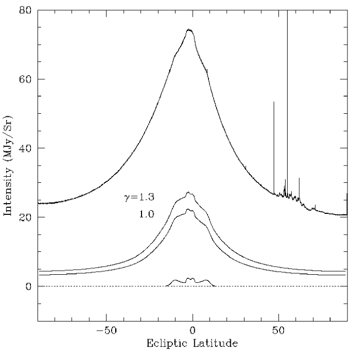
A little over fifteen years ago, the phenomenon of the zodiacal light was attributed to a smooth, lenticular distribution of cometary debris, centered on the Sun, lying in the plane of the ecliptic (see Giese et. al 1986 for a review). However, the launch of IRAS in 1983 revolutionized our knowledge of the interplanetary medium. For the first time, brightness profiles of the zodiacal cloud became available which clearly showed a level of structure, particularly near the ecliptic, which could not be explained by the previous paradigm. Figure 1 shows such a brightness profile of the zodiacal cloud, along with the results of passing the profile through a fast Fourier filter to isolate the near-ecliptic features. These features appear as ‘shoulders’ superimposed on the background emission at roughly , and a ‘cap’ near the ecliptic plane. In the discovery paper, Low et. al (1984) suggest that these dust bands are traces of collisional debris within the main asteroid belt, based on a determination of their color temperature. This is an important point: the traditional source of the interplanetary dust complex was assumed to be the debris of short period comets (Whipple 1967; Dohnanyi 1976). Although asteroid collisions should inject at least some material into the cloud, the lack of observational constraints had otherwise made the contribution of asteroidal material next to impossible to estimate.
A dust band is a toroidal distribution of dust particles with common inclinations. The dust particles themselves are asteroidal collisional debris. Particles in cometary type orbits have high orbital eccentricities; planetary gravitational perturbations produce large variations in these eccentricities and these variations are coupled to those in the inclinations (Liou et al. 1995). Therefore even if a group of cometary type orbits initally had identical inclinations, planetary perturbations would disperse those inclinations over a wide range on a timescale of a few precession periods, showing that it is impossible for a comet to produce a well defined dust band.
A given asteroid undergoing a collision will break up producing debris according to some size-frequency distribution. This distribution can be defined by the equation,
| (1) |
where is the diameter of the particle. For a system in collisional equilibrium, q=11/6 (Dohnanyi 1969) and the distribution is dominated by small particles. Assuming the excess velocities after escape are small compared with the mean orbital speed of an asteroid (15-20 km/s), the orbits of individual fragments will be similar as their orbital elements will be only slightly perturbed from those of the parent asteroid (Davis et al. 1979). Even a small initial distribution in relative velocity (10-100 m/s), corresponding to a minor dispersion in semimajor axis (0.1-1%) rapidly produces a ring of material over the parent asteroid’s orbit (102-103 years). Secular precession acts upon the particles’ longitude of ascending node due to the effect of Jovian perturbations. To first order,
| (2) |
where is the longitude of node, is Jupiter’s mass, is the Sun’s mass, is the mean orbital distance of Jupiter (5.2 AU), is the semimajor axis of a given particle and is the gravitational constant (Sykes and Greenberg 1986). The rate of nodal regression is found from the derivative of the above equation,
| (3) |
The time taken to distribute the nodes around the ecliptic to form a dust band is then given by
| (4) |
For a collisional event at 2.2 AU with ejection velocities of 100 m/s, a dust band would form after approximately 2 x 10⁶ years. Now since particles in inclined orbits spend a disproportionate amount of time at the extremes of their vertical harmonic oscillations, a set of such orbits with randomly distributed nodes will give rise to two apparent bands of particles symmetrically placed above and below the mean plane of the system (Neugebauer et al. 1984). This gives a natural explanation for the ‘shoulders’ on the IRAS profiles at approximately . Similarly, the central ‘cap’ may be simply explained as a low inclination dust band. Any dispersion in the proper inclinations of the dust particles will lead to the dust band profile appearing broader, with the peak intensity shifted to a lower latitude (Dermott et al. 1990, Grogan et al. 1997).
A point of debate in the literature rests on whether the dust bands are equilibrium or non-equilibrium features. In other words, are the dust bands produced by a gradual grinding down of asteroid family members, or do they represent regions of random, catastrophic disruptions in the asteroid belt? The equilibrium model, first discussed by Dermott et al. (1984) and most recently by Grogan et al. (1997), observes that the positions of the dust bands follow the locations of the major Hirayama asteroid families. This would be the natural consequence if the local volume density of dust, produced from continual asteroid erosion, followed the local volume density of asteroids. The catastrophic model follows from a discussion of dust band production rates (assuming the random disruption of a small single asteroid of approximately 15km diameter) and dust band lifetimes (material will be removed by Poynting-Robertson (P-R) drag). Following this logic Sykes and Greenberg (1986) conclude that several dust bands should be visible at any given time. This is in agreement with the IRAS observations and represents the main argument for the non-equilibrium model. The question is an important one to answer, and has implications for the investigation of the long-term evolution of the asteroid belt. If the equilibrium model proves correct, then the dust bands can be used as probes of collisional activity within their corresponding families and ultimately employed to estimate the percentage contribution of asteroidal material to the zodiacal dust complex. If the catastrophic paradigm is correct, then individual dust band features cannot be related to given asteroids in the belt with any confidence, and the question of the asteroidal contribution to the cloud will be much more difficult to unravel.
2 IRAS Observations of the Dust Bands
Dust band structures are not observed independently from the rest of the zodiacal cloud. The IRAS observations consist of a series of line of sight brightness profiles taken through the zodiacal cloud as a whole and to study the bands they must somehow be isolated from the remainder of the cloud. Various techniques have been employed in the literature for this purpose. Sykes (1990) uses a boxcar averaging method: this process averages data values over a given filter width (latitude bin) and subtracts that average from the central sample value. The filter is then shifted by one sample and the process repeated. This has the effect of smoothing the data, and the difference between the original data and the smoothed data gives the residuals which are then associated with the dust bands. Reach (1992) and Jones and Rowan-Robinson (1993) assume some empirical form for the background component, and subtract this from the observations to produce residuals which can then be associated with the dust bands. Finally, Fourier analysis has been employed (Dermott et al. 1986, Sykes 1988, Grogan et al. 1997, Reach et al. 1997) where a smooth low frequency background is separated from the high frequency dust band residuals.
In this paper, the dust band residuals will be obtained by means of a fast Fourier filter. This filter is sampled at an equal number of points as the number of data points in the brightness profile. The frequency cut-off is defined by a simple coefficient , a number which varies from 0 to 1 to represent the fraction of frequency points to remain after the high frequencies are stripped from the Fourier transform. In other words, defining this coefficient equal to 1 would leave the complete Fourier transform intact. Figure 2 demonstrates how more and more of the original profile is incorporated into the low frequency background as the constant increases. This is a dramatic illustration of the arbitrary nature of any filtering process and the danger of assuming the resultant residuals to represent the complete dust band structure.
The viewing geometry of the IRAS spacecraft was ideal for the study of the zodiacal cloud. The Medium Resolution (2’ in scan) Zodiacal Observational History File (ZOHF) consists of 5757 sky brightness profiles, each providing a detailed view of the pole-to-pole cloud structure in a given line of sight defined by the ecliptic longitude of Earth, with most scans being taken at around 90∘ solar elongation. Towards the end of the survey the satellite covered elongation angles between 60∘ and 120∘, but most of these observations were contaminated by Galactic emission as the Galactic plane was at this point close to the ecliptic. The changes in shape and amplitude of the dust band residuals from profile to profile are caused by a combination of the complex three-dimensional structure of the dust bands themselves and also the observing geometry of the IRAS satellite.
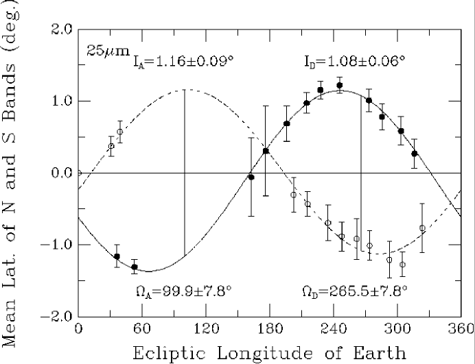
The two primary causes for a change in the line of sight are (1) the longitude of Earth and (2) the solar elongation angle. The changes due to these two parameters are taken to be independent to first order, allowing a quantitative parameter to be associated with each. Changes in elongation angle produce a parallax effect: there is a change in the effective distance to the bands, and for small changes in elongation angle the effect can be assumed to be linear. The slope for the change in peak latitude of the north or south dust band or with elongation angle can be found from a number of scans of a given longitude of Earth with varying solar elongation and this used to normalize the peak latitude that would be observed at a solar elongation of 90∘ (an example is shown in Figure 3 for a longitude of Earth of 227.3∘, trailing direction). Once this has been done, the normalized values of and may be used to obtain , the mean north/south peak latitude, which may be plotted as a function of ecliptic longitude of Earth. This is shown in Figure 4 for the ten degree band in the 25 waveband. The sinusoidal variation indicates that the plane of symmetry of the bands, the plane about which on average the proper inclinations of the particles precess, is inclined to the ecliptic. This tilt of the plane of symmetry is due to the secular perturbations of the planets, and its orientation depends on the forced elements imposed on the dust particles. When viewed from Earth such a plane would appear as a sine curve, its amplitude equal to the inclination of the plane. Also, the displacement from the ecliptic will be equal in the trailing and leading directions at the ascending and descending nodes. Profiles of different longitudes of Earth can now be coadded using the parameters of the sine curve representing the peak latitude of the bands due to their plane of symmetry being inclined to the ecliptic; this effect translates into a lateral shift that can be positive or negative depending on the longitude of Earth, and a minimum when Earth is at the forced nodes.
Individual IRAS scans were Fourier filtered and the dust band residuals coadded in the above manner to produce several representative profiles around the sky normalized to a solar elongation angle of 90∘ with noise levels an order of magnitude less than the original scans. The results of this process for the 12, 25 and 60 wavebands, leading and trailing, are shown in Figures 5-7. The dust band emission peaks in the 25 waveband, although the bands are still clearly visible at 12 and 60 . The dust bands have a lower amplitude but similar shape at 12 compared to 25 , whereas at 60 the central band is less prominent with respect to the ten degree band, an effect which is largely due to the filtering process. These observations contain a wealth of information about the structure of the dust bands; certain aspects, however, deserve special mention. Firstly, there exists a sinusoidal variation in the latitudes of peak brightness of the north and south ten degree band pair around the sky. This is due to the forced inclinations imposed on the dust band particle orbits by planetary gravitational perturbations as described above. Secondly there is a clear split in the central band and the amplitudes of each peak vary around the sky. The amplitudes of the north and south ten degree band pair also undergo such a variation except that this variation seems to be out of phase with the variation seen in the corresponding north and south peaks of the central band. The complex structure revealed by these observations underlines the point that empirical models which attempt the describe the zodiacal cloud as a whole will always fall short in accounting for features such as these, and the problem demands a detailed dynamical treatment.
3 A Physical Model for the Dust Bands
The legacy of the IRAS, COBE and ULYSSES spacecraft is a realization that the zodiacal cloud may consist of five distinct and significant components. These are (1) the asteroidal dust bands (Dermott et al. 1984; Sykes and Greenberg 1986; Reach 1992; Grogan et al. 1997), (2) dust associated with other background (non-family) asteroids, (Dermott et al. 1994a) (3) dust associated with cometary debris (Sykes and Walker 1992; Liou and Dermott 1995), (4) the Earth’s resonant ring (Dermott et al 1994b), and (5) interstellar dust (Grun et al. 1994; Grogan et al. 1996). It is also possible that a significant proportion of interplanetary dust particles originate in the Kuiper belt (Flynn 1996, Liou et al. 1996). The approach of the Florida group (Dermott et. al) has been to place constraints on the origin and evolution of material of a given source from both dynamical considerations and observational data. Given a postulated source of particles, the aim is to describe (1) the orbital evolution of these particles, including P-R drag, using equations of motion that include the solar wind, light pressure and planetary gravitational perturbations, and (2) the thermal and optical properties of the particles and their variation with particle size. Once the dust particles and their distribution have been specified along these lines, a line-of-sight integrator is employed to not only view the model cloud but to reproduce the exact viewing geometry of any particular telescope in any given waveband. The result is a series of model profiles which can then be compared with observations.
Amongst the various forces acting upon the dust particles the most obvious is solar gravity,
| (5) |
where is the gravitational constant and is the solar mass. Scattering and absorption of solar radiation by a dust particle involve the transfer of momentum and hence to a radiation pressure directed radially outwards (Burns et al. 1979). For spherical particles radiation pressure takes the value
| (6) |
where is the radiation flux density at distance , is the solar luminosity and is an efficiency factor averaged over the solar spectrum which can be calculated using, for example, Mie theory (Bohren and Huffman, 1983). Radiation pressure is usually expressed as the ratio of its strength to the gravitational attraction, which for spherical particles is given by
| (7) |
where is the particle radius and and are given in cgs units. Roughly speaking, radiation pressure balances gravity for a 1 m particle. The component of radiation pressure tangential to the particle orbit gives rise to the phenomenon known as Poynting-Robertson (P-R) drag, which results in an evolutionary decrease in both the semi-major axis and eccentricity of the particle orbit. These changes in the orbital elements can be given by
| (8) |
| (9) |
| (10) |
where
| (11) |
(Wyatt and Whipple 1950). The consequence is that the orbit shrinks and circularizes, and a particle in a circular orbit at heliocentric distance spirals into the Sun in a time
| (12) |
This equates to several years for a ‘typical’ particle (10 m, 2.5 g/cm3, initial =2 AU).
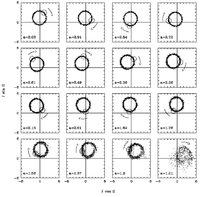
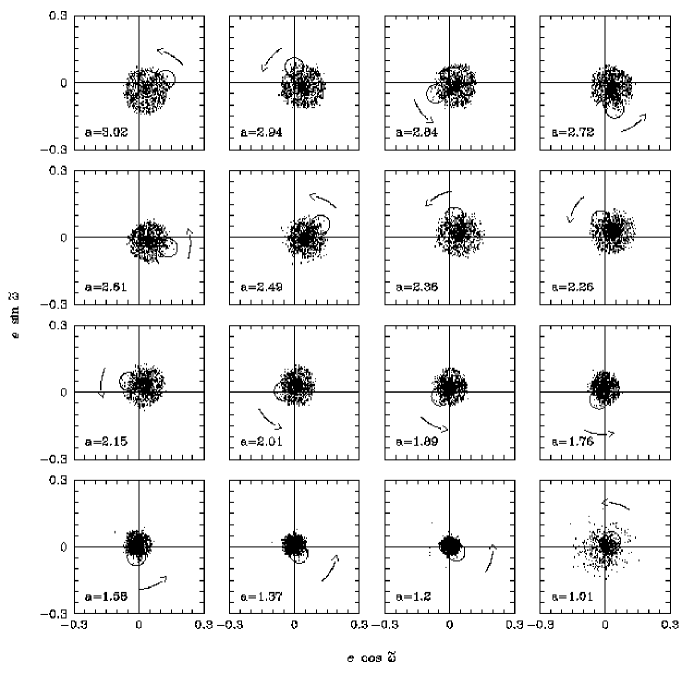
Now consider the motion of dust particles under the effects of planetary gravitational perturbations. When the eccentricity and inclination are small, the solutions of the Lagrangian equations of motion for the eccentricity and pericenter variations may be completely decoupled from the inclination and node variations. These pairs of elements have simple vectorial representations and may be decomposed into components known as the proper elements and the forced elements of the orbit. The proper elements represent the stable long-term averages that remain after removal of planetary perturbations. The variations due to these perturbations are the forced elements, which can themselves be separated into three categories: (1) secular (long period) perturbations; (2) resonant (short period) perturbations; (3) transient (scattering) perturbations. These perturbations acting on a small body in orbit about the Sun precess the node and pericenter and over sufficiently long intervals the distributions of these elements become essentially random. Figure 8 shows a schematic of the vectorial relationship between the total (osculating) elements (, ), the proper elements (, ) and the forced elements (, ) in ( cos , sin ) space. The distribution is displaced from the origin due to the forced elements and the radius of the distribution represents the proper elements. An equivalent relationship exists for eccentricity and pericenter. Figures 9 and 10 show the evolution of 249 Koronis dust particles migrating from the asteroid belt toward the Sun (Kortenkamp and Dermott 1998). Secular perturbations, primarily from Jupiter and Saturn, vary with time and semi-major axis and act to change the forced elements of the distribution as the wave migrates into the inner Solar System. The orbital eccentricities also decay due to P-R drag and solar wind drag.
Dermott et al. (1984) were the first to suggest that the Solar System dust bands may originate in the three prominent Hirayama asteroid families (Eos, Themis and Koronis). To confirm their hypothesis of the asteroidal origin of the dust bands, and to facilitate the investigation of the zodiacal cloud in general, SIMUL, a three-dimensional numerical model was constructed (Dermott et al. 1988). The basic ideas and assumptions behind SIMUL are as follows.
-
1.
A cloud is represented by a large number of dust particle orbits. The total cross-sectional area of the cloud is divided equally among all the orbits.
-
2.
The orbital elements of the dust particle orbits in the cloud can be decomposed into proper and forced vectorial components. When inclination and eccentricity are low, as is typically the case for asteroidal type orbits, at any given time the forced elements are independent of the proper elements and depend only on the semimajor axis and the particle size.
-
3.
As a first approximation, the dust particles in the cloud produced by asteroid families have the same mean proper elements as those of the parent bodies, although the Gaussian distribution of these elements is a free parameter.
-
4.
The forced elements as a function of semimajor axis are calculated using secular perturbation theory via direct numerical integrations, as outlined above.
-
5.
Along each of the orbits, particles are distributed according to Kepler’s Law. Once the spatial distribution of the orbits is specified, space is divided into a sufficiently large number of ordered cells and then every orbit is investigated for all the possible cross-sectional area contributions to each of the space cells. The model generates a large three-dimensional array which serves to describe the spatial distribution of the effective cross-sectional area.
-
6.
The viewing geometry of any telescope can be reproduced exactly by calculating the Sun-Earth distance and ecliptic longitude of Earth at the observing time and setting up appropriate coordinate systems. In this way, IRAS-type brightness profiles can be created and compared with the observed profiles.
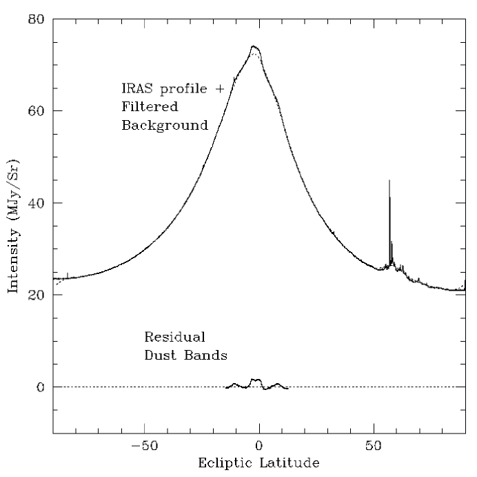
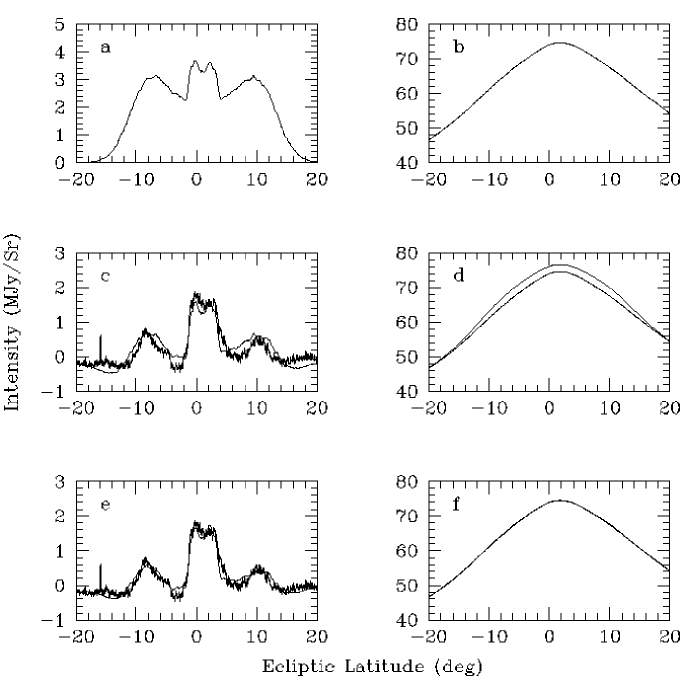
In order to compare the results of the SIMUL modeling algorithm with the IRAS observations, the filtering problem - the fact that a substantial percentage of the dust band signal is indistinguishable from the background - must be addressed. An iterative process (Dermott et al. 1994a, Grogan et al. 1997) is used to determine the low-frequency component of the dust band and therefore bypass this filtering problem. Figure 11 shows how this is achieved. Panel (a) shows a raw model dust band having the same viewing geometry as an observed background, produced by filtering off the high-frequency dust band component. In the first iteration (a) is added to (b) and the sum is filtered to obtain (c), a filtered model dust band (smooth curve) - the observed dust bands (noisy curve) are also plotted for comparison. The background obtained from this iteration, shown in panel (d) is of a higher intensity than the original background due to the fact that it contains two low-frequency dust band components, one from the addition of the model dust band and one from the actual dust band in the original observed background (the high frequency component of which was removed in the creation of the observed background). In other words, the difference between these two backgrounds gives the extent of the low-frequency dust band component. In the final iteration we subtract the excess intensity shown in panel (d) from the original background (b) and add (a) before filtering to obtain the final dust band model (e) and the final background (f) that agree with the observations. Thus, by using the same filter in the modeling process that we use to define the observed dust bands, and iterating, we are able to bypass the arbitrary divide associated with the filter.
4 Results
This work differs from our previous modeling of the dust bands (Grogan et al. 1997) in that our models include a size-frequency distribution, rather than being composed of particles of a single size. This is critical in our efforts to provide a model of the dust bands that can match the IRAS observations in multiple wavebands. Particles ranging in size from 1 to 100 are included, each of which are assumed to be Mie spheres composed of astronomical silicate (Draine and Lee 1984). The lower end cut-off is determined by the fact that contribution to the thermal emission from particles smaller than this size is negligible. The upper cut-off follows from the fact that in the zodiacal cloud, the P-R drag lifetime is comparable to the collisional lifetime for a particle of about this size (Leinert and Grün 1990). However, the inclusion of a wide range of particle sizes can only be achieved with an understanding of their dynamical history, so that their orbital distributions can be properly described in the SIMUL algorithm. This is achieved using the RADAU fifteenth order integrator program with variable time steps taken at Gauss-Radau spacing (Everhart 1985), with which we perform direct numerical integration of the full equations of motion of interplanetary dust particles (IDPs) of various sizes. Our simulations include seven planets (Mercury and Pluto excluded) and account for both P-R drag and solar wind drag. The average force due to the solar wind drag is taken to be 30% of the P-R drag force, varying with the 11-year solar cycle from 20% to 40% (Gustafson 1994). In this way we are able to build a description of both the proper and forced elements of the particles and their variation with heliocentric distance from their simple vectorial relationship shown in Figure 8. Because the forced elements vary as a function not only of semi-major axis but also of time, each wave of particles (as shown in Figures 9 and 10) is started at different times in the past, such that when the waves reach the present they span the full range of semi-major axis from the asteroid belt into the Sun. In this way a snapshot of the present day forced element distribution is constructed. Figure 12 shows the variation with heliocentric distance of the forced inclination (top) and forced longitude of ascending node (bottom) of 4, 9, 14, 25 and 100 diameter IDPs in the zodiacal cloud. As the particle size increases, its P-R drag lifetime increases and it therefore spends longer in secular resonances near the inner edge of the asteroid belt. This causes the forced inclination of a 100 micron diameter particle to approach 6∘ interior to 2 AU. An equivalent diagram for the forced eccentricity and forced pericenter is shown in Figure 13.
Dust band models are produced via SIMUL in the following manner.
-
1.
A model to account for the central band is created by using two distributions of orbits having mean semi-major axis, proper eccentricity, proper inclination and dispersions equal to those found in the Themis and Koronis families. The proper elements found from the numerical integrations are added vectorially to find the osculating orbital elements, and the material is distributed into the inner Solar System as far as 2 AU according to P-R drag (a , distribution). The size-frequency distribution of material in the observed dust band is investigated by varying the size-frequency index of particles in the model.
-
2.
A model to account for the ten degree band is created from Eos type orbits, in that their mean semi-major axis and eccentricity are equal to those found in the Eos families. However, in order to improve upon previous modeling of the ten degree band the mean proper inclination of the distribution was allowed to vary within the range of proper inclinations found in the Eos family. A best fit was found at a mean proper inclination of 9.35∘ with a dispersion of 1.5∘. Again, the proper elements are added vectorially, the material distributed into the inner Solar System as far as 2 AU, and a size-frequency distribution applied.
-
3.
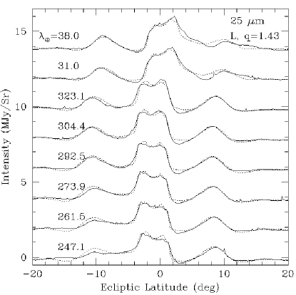
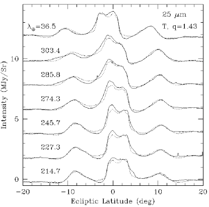
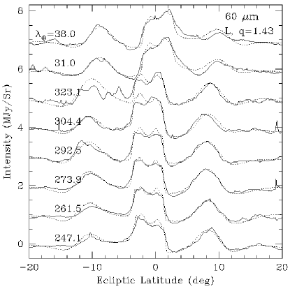
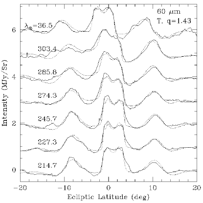
We do not create a model for the zodiacal background but instead add the model dust band profiles to the observed background obtained from applying the Fourier filter to the corresponding raw IRAS observation. The total is then filtered using the iterative procedure described above so that the resultant model residual can be directly compared with the observed dust bands. For a given size-frequency index , the total surface area of material associated with the model bands is adjusted until the amplitudes of the 25 model dust bands matches the 25 observations; can then be varied until a single model provides a match in amplitude to the 12, 25 and 60 observations simultaneously.
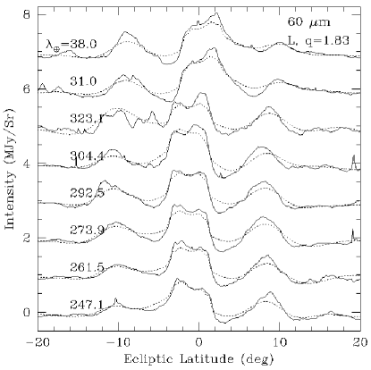
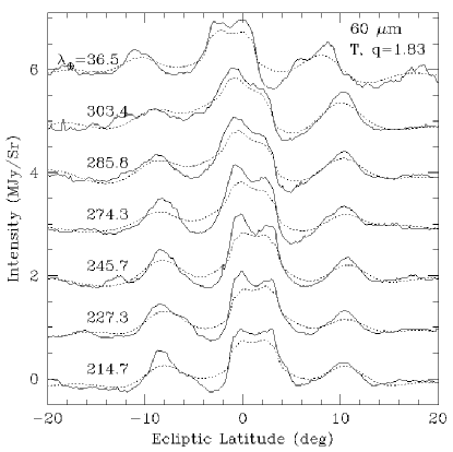
Figures 14-16 show the best results of our modeling, comparing the dust band observations (solid curves) to the dust band models (dotted curves) in the 12, 25 and 60 wavebands. The models were constructed as described above, and have a size-frequency index equal to 1.43. Large particles dominate this distribution. Table 1 lists the parameters used in the model components. The amplitudes in all wavebands are well matched, and the shapes of the dust band models describe the variation in shape of the observations around the sky very well. Figure 17 shows how the goodness of fit of our models changes as a function of size-frequency index for a single longitude of Earth. This has been obtained for the ten degree band by calculating the root mean square (observation - model) over two five degree wide latitude bins to cover the north and south bands for both the 12 and 60 micron wavebands. In essence, the wavebands act as filters through which different particle sizes in the cloud are seen. The 12 waveband preferentially detects emission from the smaller particles, and the 60 waveband preferentially detects emission from the larger particles. Therefore,
-
1.
When is too high, too many small particles are included in the model, and the ampitudes of the 12 models are too large. In addition, too few large particles are included and the amplitudes of the 60 models are too small. This effect can be seen in Figures 18-19, in which dust band models have been produced with =1.83, appropriate for a system in collisional equilibrium.
-
2.
When is too low, too many large particles are included in the model. This leads to the distribution of forced inclinations in the model to be skewed too much towards the large end, and the model profiles are shifted in latitude with respect to the observations, degrading the fit. This effect is much smaller than the amplitude effect for high , and will only be properly quantified when a fuller description of the action of large particles at the 2 AU secular resonance has been produced.
A clear result is that a high size-frequency index , in which small particles dominate, fails to account for the observations of the Solar System dust bands. This index has to be reduced to the point where large particles dominate the distribution. This is consistent with the cratering record on the LDEF satellite, shown in Figure 20, which suggests a of approximately 1.15 at Earth and a peak in the particle diameter at around 100-200 micron. Since the Fourier filter preferentially isolates material exterior to the 2 AU secular resonance (in the inner Solar System the dust band material is dispersed into the background cloud due to the action of secular resonances), our results are more indicative of the size-frequency index of dust in the asteroid belt. We do not mean to claim that the size-frequency index is a constant throughout the main-belt: the true nature of the distribution will be a complex function of dust production rates, P-R drag rates, collisional lifetimes and the nature of particle-particle collisions. Consequently, the size distribution will presumably be some function of heliocentric distance. However, in describing in main belt region as a whole, we do claim that large particles appear to dominate the dust band emission over small particles.
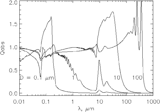
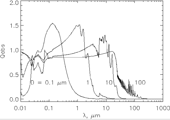
One concern that must be addressed is the possibility that the observed relative amplitudes of the dust band material are driven by the optical properties of the dust particles, and not the size-frequency index. For this reason, we have repeated the modeling process assuming the particles to be made of organic refactory material (Li and Greenberg 1997). Figure 21 shows the variation with wavelength and particle diameter of the absorption efficiencies of both astronomical silicate (top) and organic refractory material (bottom), calculated using Mie theory. One striking difference between the two, particularly relevant for this discussion, is that emission at longer wavelengths for large particles is highly attenuated for the organic refractory material compared to the astronomical silicates. Figure 22 shows how the residuals obtained in the modeling process are affected by the change in the composition of the dust particle. The 12 micron residuals strongly reinforce the result obtained with astronomical silicate that a low size-frequency index is required to match the observations. The evidence at 60 micron is less clear, where we are hindered by the low emissivity of this material at longer wavelengths for larger particles. Even so, the residuals are decreasing with decreasing . The consistent picture is that the dust band distribution is dominated by particles at the large end of the size range.
5 Discussion
The results presented in this paper improve upon those reported in a previous paper (Grogan et al. 1997), particularly in regard to the ten degree band associated with the Eos family. In order for a dust band model to match the observations, it needs to fit both the latitude of peak flux (driven by the mean proper inclination of the particles) and the width of the dust band feature (a function of the dispersion in proper inclinations). Previously, the dispersion in proper inclinations of the Eos dust particles was reported at a relatively high 2.5∘, which minimized the residuals while the mean proper inclination of the particles was fixed at the mean proper inclination of the Eos asteroid family. In this paper, smaller residuals are found when the mean proper inclination of the particles is allowed to float as a free parameter; the best fit then corresponds to a mean proper inclination of 9.35∘ and a dispersion of only 1.5∘.
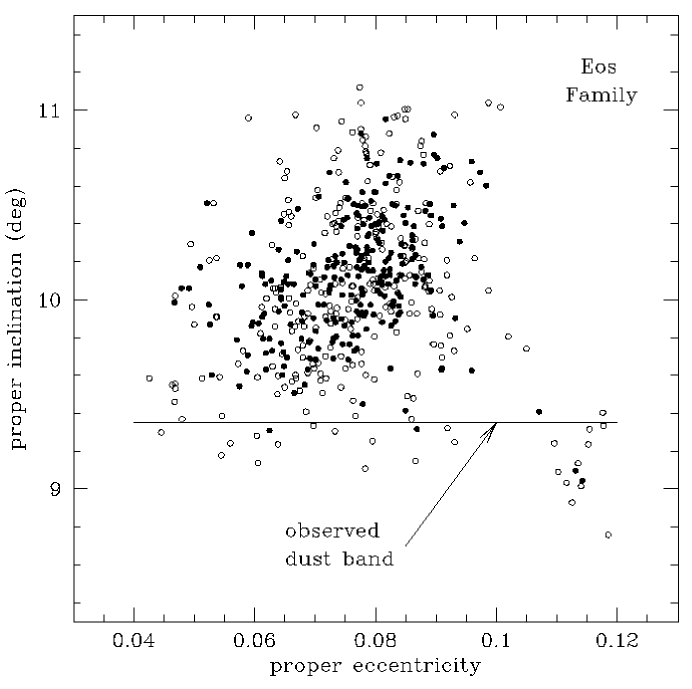
Figure 23 shows the members of the Eos asteroid family in (e,i) space as determined by the hierarchical clustering method (Zappala et al. 1995). Shown on this diagram is the position of the mean proper inclination of the ten degree band model. The consequence is that the ten degree dust band material is not tracing the orbital element space of the Eos family as a whole, as would perhaps be expected from the equilibrium model. Either the collisional activity is occurring near the inner edge of the Eos family, or the inclinations of dust particle orbits originating from the Eos family as a whole no longer trace the inclinations of their parent bodies but have been degraded since their production. If some mechanism was degrading the dust particle orbits it would presumably apply to particles from all sources, but may be more easily observed within the Eos family owing to its high inclination. Trulsen and Wikan (1980) have suggested based on their numerical simulations that the combined influence of P-R drag and collisions acts to decrease both the mean eccentricity and inclination of dust particle orbits. This subject is however open to debate; the nature of collisions between interplanetary dust particles is still poorly understood. Figure 24 shows the cumulative surface area as a function of different size-frequency distrubtion indices for the Eos, Themis and Koronis families and also a single 15km diameter asteroid. At first this appears to contradict our result that a low of around 1.43 is needed to model the dust bands. However, the diagram is set up such that size-frequency distribution is constant from the source point all the way down to the smallest IDPs, which we know is not the case since P-R drag will act to preferentially remove the small particles. In reality, the size-frequency distribution will change from the large to the small end of the distribution, and will also be a function of heliocentric distance. The diagram does suggest that for a single asteroid to be responsible for the ten degree dust band, the size-frequency index of the collisional debris would initially have needed to be extremely high to produce the surface area required to match the observations.
The justification of cutting off the distribution of dust band material at 2 AU is essentially given by Figure 12. As the particles move out of the asteroid belt the action of the secular resonance disperses them into the background cloud, an effect which is more marked as the particle size increases. For this reason the Fourier filter is particularly sensitive to material located in the asteroid belt, and models that confine the material to the asteroid belt match the observations very well. In the future, our models will populate the inner Solar System as well as the main-belt region, but to do this properly we will have to:
-
1.
Investigate the dynamical history of a much greater number of particle sizes than the five sizes we have considered so far in order to properly account for their behavior at the 2 AU secular resonance;
-
2.
Take into account collisional processes: larger particles will have shorter collisional lifetimes compared to their P-R drag lifetimes and will therefore not penetrate as far into the inner Solar System. Each distribution of orbits of a given particle size will therefore have a natural inner edge defined by the lifetime of the particles in the cloud.
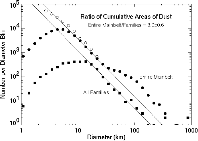
However, we can obtain an estimate for the dust band contribution to the zodaical cloud as a whole by simply extending our best fit dust band models to populate the inner Solar System. The distribution of orbits obtained in this manner will not be exactly correct, due to our insufficient treatment of the secular resonance, but will still be reasonably accurate in terms of the total surface area associated with the dust bands. Figure 25 compares the thermal emission obtained from this raw dust band model to the corresponding IRAS profile in the 25 waveband. The result is shown for inner Solar System distributions of material corresponding to =1.0, as expected for a system evolved by P-R drag, and =1.3 as predicted in parametric models of the zodiacal cloud, most recently Kelsall et al. (1998). The dust bands appear to contribute approximately 30% to the total thermal emission. Also shown is the amplitude of the dust band material confined to the main belt (exterior to 2 AU), which represents the component of the dust band material isolated by the fast Fourier filter. This clearly shows the extent to which the dust band contribution is underestimated if it is assumed that the filtered dust band observations represent the entirety of the dust band component of the cloud. Figure 26 shows the ratio of areas of material associated with the entire main belt asteroid population and all families, for asteroid diameters greater than 1 km. The best fit lines have a slope corresponding to a size-frequency index . This diagram can be used to estimate the total contribution of main belt asteroid collisions to the dust in the zodiacal cloud, by extrapolating the observed size distributions of larger asteroids in both populations assuming a collisional equilibrium power law size distribution. The result is that the main belt asteroid population contributes approximately three times the dust area of the Hirayama families alone, and the total asteroidal contribution to the zodiacal cloud could account for almost the entireity of the interplanetary dust complex. In reality, evolved size distributions are more complex than simple power laws (Durda et al. 1998) and the size distribution of individual asteroid families likely preserve some signatures of the original fragmentation events from which they were formed. However, small dust-size particles and their immediate parent bodies have collisional lifetimes in the main belt that are considerably shorter than the age of the Solar System or the major asteroid families. Thus the dust size distributions associated with both the background main belt and family asteroids may well be considered to have achieved an equilibrium state, with total areas related to the equivalent volumes of the original source bodies in each population. An alternative, and perhaps more satisfactory, approach to obtaining the total asteroidal contribution to the zodiacal cloud will be to apply our methods to the main-belt asteroid population in the same way we have investigated the dust bands. This is the subject of a future paper.
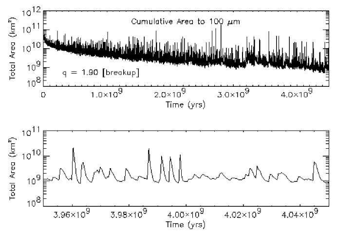
The origin of the large dispersion in proper inclination (1.5∘) required to successfully model the ten degree band, in rough agreement with the 1.4∘ found by Sykes (1990) and the 2∘ found by Reach et al. (1997), remains unclear. Dispersion in inclination due to the Lorentz force is expected to behave such that the root mean square of the dispersion will increase with the square root of the distance traveled, and will be inversely proportional to the cube of the radius of the particle (Leinert and Grün 1990). Morfill and Grün (1979) report a value of only 0.3∘ for a particle of 1 radius by the time it has spiraled in to 1 AU from the asteroid belt after 3000 years, with that expected for a 100 micron particle to be significantly less. Subsequent treatments by Consomagno (1979), Barge et al. (1982) and Wallis and Hassan (1985) differ by more than an order of magnitude due to the lack of detailed knowledge of the magnetic field structure. A more likely source of the dispersion is simply the action of the secular resonance at 2 AU. However, this leaves open the question of why a large dispersion is required to model the ten degree band, and only the small dispersion of the Themis and Koronis families is required to successfully reproduce the central band observations. One answer may be that the emission associated with the central band is due to relatively recent collisions within these families. Figure 27 shows the variation with time of the total cross-sectional area associated with the main belt and describes the stochastic breakup of asteroidal fragments. This numerical approach to describing the collisional evolution of the asteroid belt is detailed by Durda and Dermott (1997). The initial main belt mass is taken to be approximately three times greater than the present mass (Durda et al. 1998); this population evolves after 4.5 Gyr to resemble the current main belt. The calculation is performed for particles from 100 through the largest asteroidal sizes, with a fragmentation index . The dust production rate in the main asteroid belt becomes more stochastic with time following a relatively smooth decrease in area as the small particles are created directly from the breakup of the parent body are destroyed. The spikes in the dust production are due to the breakup of small to intermediate size asteroids. Therefore while the observable volume of a family may decay at a fairly constant and well-defined rate, the total area of dust associated with the family during that time may fluctuate by an order of magnitude or more.
We have shown in this paper how the Solar System dust bands can be investigated and used as a tool for addressing fundamental questions about the nature of the zodiacal cloud and the origin of the material from which it is composed. A key component of this process has been the realization that large particles play a dominating role in the structure of the cloud and that their dynamical histories need to be included in any physically motivated model. In the future we will extend our knowledge of the dust dynamics to a wider range of particle sizes, and address the main-belt contribution as well as the dust band component on the way to our ultimate goal of providing a global model for the zodiacal emission.
References
-
Barge, P., Pellat, R. and Millet, I. 1982. Diffusion of Keplarian motions by a stochastic force. II. Lorentz scattering of interplanetary dusts. Astron. Astrophys. 115, 8-19.
-
Bohren, C.F. and Huffman, D.R. 1983. Absorption and Scattering of Light by Small Particles, Wiley, New York.
-
Burns, J.A., Lamy, P.L. and Soter, S. 1979. Radiation Forces on Small Particles in the Solar System. Icarus 40, 1-48.
-
Consomagno, G. 1979. Lorentz scattering of interplanetary dust. Icarus 38, 398-410.
-
Davis, D.R., Chapman, C.R., Greenberg, R., Weidenschilling, S.J. and Harris, A.W. 1979. Collisional evolution of asteroids. In Asteroids, ed. T. Gehrels, 528-557. Univ. of Arizona Press, Tuscon.
-
Dermott, S.F., Nicholson, P.D., Burns, J.A. and Houck, J.R. 1984. Origin of the Solar System dust bands discovered by IRAS. Nature 312, 505-509.
-
Dermott, S.F., Nicholson, P.D. and Wolven, B. 1986. Preliminary Analysis of the IRAS Solar System Dust Data. In Asteroids, Comets, Meteors II, eds. C.-I. Lagerkvist, B.A. Lindblad, H. Lundstedt and H. Rickman, 583-594, Reprocentralen HSC, Uppsala.
-
Dermott, S.F., Nicholson, P.D., Kim, Y., Wolven, B. and Tedesco, E.F 1988. The Impact of IRAS on Asteroidal Science. In Comets to Cosmology, ed. A. Lawrence, 3-18. Springer-Verlag, Berlin.
-
Dermott, S.F., Nicholson, P.D., Gomes, R.S. and Malhotra, R. 1990. Modeling the IRAS Solar System dust bands. Adv. Space Res. 10(3), 171-180.
-
Dermott, S.F., Durda, D.D., Gustafson, B.Å.S., Jayaraman, S., Liou, J.C. and Xu, Y-L. 1994a. Zodiacal Dust Bands. In Asteroids, Comets, Meteors 1993, eds. A. Milani, M. Martini and A. Cellino, 127-142. Kluwer, Dordrecht.
-
Dermott, S.F., Jayaraman, S., Xu, Y-L., Gustafson, B.Å.S. and Liou, J.C. 1994b. A circumsolar ring of asteroidal dust in resonant lock with the Earth. Nature 369, 719-723.
-
Dohnanyi, J.S. 1969. Collisional model of asteroids and their debris. J. Geophys. Res. 74, 2531-2554.
-
Dohnanyi, J.S. 1976. Sources of interplanetary dust, asteroids. In Interplanetary Dust and Zodiacal Light, Lecture Notes in Physics Vol. 48, eds. H. Elsässer and H. Fechtig, 187-205. Springer, Berlin.
-
Draine, B.T. and Lee, H.M. 1984. Optical properties of interstellar graphite and silicate grains. Ap.J 285, 89-108.
-
Durda, D.D. and Dermott, S.F. 1997. The Collisional Evolution of the Asteroid Belt and Its Contribution to the Zodiacal Cloud. Icarus 130, 140-164.
-
Durda, D.D., Greenberg, R. and Jedicke, R. 1998. Collisional Models and Scaling Laws: A New Interpretation of the Shape of the Main-Belt Asteroid Size Distribution. Icarus 135, 431-440.
-
Everhart, E. 1985. An efficient integrator that uses Gauss-Radau spacings. In Dynamics of Comets, eds. A. Carusi and G.B. Valsecchi, 185-202. Reidel, Dordrecht.
-
Flynn, G.J. 1996. Collisions in the Kuiper Belt and the Production of Interplanetary Dust Particles. Meteoritics and Planet. Sci. 31, A45.
-
Giese, R.H., Kneissel, B. and Rittich, U. 1986. Three-dimensional zodiacal cloud, a comparative study. Icarus 68, 395-411.
-
Grogan, K., Dermott, S.F. and Gustafson, B.Å.S. 1996. An Estimation of the Interstellar Contribution to the Zodiacal Thermal Emission. Ap.J 472, 812-817.
-
Grogan, K., Dermott, S.F., Jayaraman, S. and Xu, Y-L. 1997. Origin of the ten degree dust bands. Planet. Space Sci. 45, 1657-1665.
-
Grün, E., Gustafson, B.Å.S., Mann, I., Baguhl, M., Morfill, G.E., Staubach, P., Taylor, A. and Zook, H.A. 1994. Interstellar Dust in the Heliosphere. Astron. Astrophys. 286, 915-924.
-
Gustafson, B.Å.S. 1994. Physics of zodiacal dust. Ann. Rev. Earth Planet. Sci. 22, 553-595.
-
Jones, M.H. and Rowan-Robinson, M. 1993. A physical model for the IRAS zodiacal dust bands. MNRAS 264, 237-247.
-
Kelsall, T., Weiland, J.L., Franz, B.A., Reach, W.T., Arendt, R.G., Dwek, E., Freudenreich, H.T., Hauser, M.G., Moseley, S.H., Odegard, N.P., Silverberg, R.F. and Wright E.L. 1998. The COBE Diffuse Infrared Background Experiment Search for the Cosmic Infrared Background. II. Model of the Interplanetary Dust Cloud. Ap.J 508, 44-73.
-
Kortenkamp, S.J. and Dermott, S.F. 1998. Accretion of Interplanetary Dust Particles by the Earth. Icarus 135, 469-495.
-
Leinert, C. and Grün, E. 1990. Interplanetary Dust. In Space and Solar Physics, Vol. 20, Physics and Chemistry in Space: Physics of the Inner Heliosphere I, eds. R. Schween and E. Marsch, 207-275. Springer, Berlin.
-
Li, A. and Greenberg, J.M. 1997. A unified model of interstellar dust. Astron. Astrophys. 331, 566-584.
-
Liou, J.C., Dermott, S.F. and Xu, Y-L. 1995. The contribution of cometary dust to the zodiacal cloud. Planet. Space Sci. 43, 717-722.
-
Liou, J.C., Zook, H.A. and Dermott, S.F. 1996. Kuiper Belt Dust Grains as a Source of Interplanetary Dust Particles. Icarus 124, 429-440.
-
Low, F.J., Beintema, D.A., Gautier, T.N., Gillet, F.C., Beichmann, C.A., Neugebauer, G., Young, E., Aumann, H.H., Boggess, N., Emerson, J.P., Habing, H.J., Hauser, M.G., Houck, J.R., Rowan-Robinson, M., Soifer, B.T., Walker, R.G. and Wesselius, P.R. 1984. Infrared Cirrus: New Components of the Extended Infrared Emission. Ap.J 278, L19-L22.
-
Morfill, G.E. and Grün, E. 1979. The motion of charged dust particles in interplanetary space. I. The zodiacal dust cloud. Planet. Space Sci. 27, 1269-1282.
-
Neugebauer, G., Beichman, C.A., Soifer, B.T., Aumann, H.H., Chester, T.J., Gautier, T.N., Gillett, F.C., Hauser, M.G., Houck, J.R., Lonsdale, C.J., Low, F.J. and Young, E.T. 1984. Early results from the infrared astronomical satellite. Science 224, 14-21.
-
Reach, W.T. 1992. Zodiacal Emission III. Dust Near The Asteroid Belt. Ap.J 392, 289-299.
-
Reach, W.T., Franz, B.A. and Weiland, J.L. 1997. The Three-Dimensional Structure of the Zodiacal Dust Bands. Icarus 127, 461-484.
-
Sykes, M.V. 1988. IRAS Observations of Extended Zodiacal Structures. Ap.J 334, L55-L58.
-
Sykes, M.V. 1990. Zodiacal Dust Bands: Their Relation to Asteroid Families. Icarus 84, 267-289.
-
Sykes, M.V. and Greenberg, R. 1986. The Formation and Origin of the IRAS Zodiacal Dust Bands as a Consequence of Single Collisions between Asteroids. Icarus 65, 51-69.
-
Sykes, M.V. and Walker, R.G. 1992. Cometary dust trails. I - Survey. Icarus 95, 180-210.
-
Trulsen, J. and Wikan, A. 1980. Numerical Simulation of Poynting-Robertson and Collisional Effects in the Interplanetary Dust Cloud. Astron. Astrophys. 91, 155-160.
-
Wallis, M.K. and Hassan, M.H.A. 1985. Stochastic diffusion of interplanetary dust grains orbiting under Poynting-Robertson forces. Astron. Astrophys. 151, 435-441.
-
Whipple, F.L. 1967. On maintaining the meteoritic complex. Smithsonian Astrophysical Observatory Special Report 239, 1-46.
-
Zappala, V., Bendjoya, P.H., Cellino, A., Farinella, P. and Froeschle, C. 1995. Asteroid families: Search of a 12,487 asteroid sample using two different clustering techniques. Icarus 116, 291-314.
Table 1
| Asteroid family | Area | |||
|---|---|---|---|---|
| Eos | 3.015, 0.012 | 0.076, 0.009 | 9.35, 1.5 | 4.0 |
| Themis | 3.148, 0.035 | 0.155, 0.013 | 1.43, 0.32 | 0.35 |
| Koronis | 2.876, 0.026 | 0.047, 0.006 | 2.11, 0.09 | 0.35 |


 |
 |
 |
 |
 |
 |

 |
 |
 |
 |
 |
 |
 |
 |
 |
 |

 |
 |
 |
 |

 |
 |

 |
 |
 |
 |